Double Markov Random Fields and
Bayesian Image Segmentation
Dina E. Melas and Simon P. Wilson
Abstract—Markov random fields are used extensively in
model-based approaches to image segmentation and, under the Bayesian paradigm, are implemented through Markov chain Monte Carlo (MCMC) methods. In this paper, we describe a class of such models (the double Markov random field) for images composed of several textures, which we consider to be the natural hierarchical model for such a task. We show how several of the Bayesian approaches in the literature can be viewed as modifications of this model, made in order to make MCMC implementation possible. From a simulation study, conclusions are made concerning the performance of these modified models.
Index Terms—Bayesian statistics, hierarchical model, image
seg-mentation, Markov random field, remote sensing.
I. INTRODUCTION
T
HE MARKOV random field has been used in many model-based solutions to image analysis problems, including that of image segmentation. In image segmentation, a digital image is to be divided into regions that are deemed to possess similar local properties, which, here, are taken to be texture. Applica-tions include• land-use estimation from satellite images; • computer-aided medical diagnosis; • content-based image retrieval; • image compression;
• recovery of shape information from an image.
We consider so-called supervised and semi-unsupervised segmentation, where the number of texture classes in the image is known but information about their properties is either known or unknown, respectively. In a Bayesian approach, the goal is to infer the posterior distribution of possible segmentations and, where necessary, any unknown model parameters. This approach is implemented through Markov chain Monte Carlo (MCMC) methods, usually the Gibbs sampler. Although computationally more expensive than many other approaches, the MCMC approach has the advantage that the analysis also yields, through the posterior distribution, information on
Manuscript received December 7, 2000; revised October 9, 2001. This work was supported by the European Science Foundation Program on Highly Struc-tured Stochastic Systems and also forms part of the work under the European Union Research Network MOUMIR. This paper was partly written while S. P. Wilson was at Projet Ariana, INRIA-Sophia Antipolis, France. The associate editor coordinating the review of this paper and approving it for publication was Prof. Simon J. Godsill.
D. E. Melas is with Interoperability Systems International, Athens, Greece (e-mail: [email protected]).
S. P. Wilson is with the Department of Statistics, Trinity College, Dublin, Ireland (e-mail: [email protected]).
Publisher Item Identifier S 1053-587X(02)00560-3.
uncertainty in the segmentation and properties of the texture classes.
There are three objectives in this paper. The first is to describe the general notion of a double Markov random field model for images composed of regions of different texture. Our contention is that this represents a natural model for the task of segmenta-tion. Our second objective is to show that many of the Markov random field models used for segmentation can be viewed as adaptations of this model so that MCMC can be used. Five such general adaptations are described. The final objective is to com-pare, by a simulation study, the performance of these adapta-tions. We conclude that one of the models seems to perform better overall than the others, and this is applied to segment a satellite image.
The paper is organized as follows. Section II defines the double Markov random field and its application to Bayesian image segmentation. Section III describes five modifications to the model to enable segmentation by MCMC. Section IV is a comparison of these modifications by a simulation study, and Section V applies the most successful model to land-use estimation from satellite radar images. Section VI completes the paper with some concluding remarks.
II. DOUBLEMARKOVRANDOMFIELD
Consider a rectangular lattice of pixel sites . An image con-sists of an array of grey values and labels , iden-tifying the texture type present. We assume that there are tex-tures in the image and that each texture, defined on all of , is a Markov random field , parameterized by , with neigh-borhood system having a set of cliques . The label process is another Markov random field , parameterized by and with neighborhood system represented by the set of cliques . All the fields are independent, conditional on model parameters, and their distributions have the following Gibbs representation:
(1)
(2)
where and are the clique potentials, and
and are the partition functions. The observed image is
(3)
where and , denote and
restricted to .
In order to evaluate , it is necessary to
iden-tify the interaction structure of pixels that have missing neigh-bors. This is generally intractable, leading to the use of various boundary assumptions. The marginal distribution on the regions is then approximated by the joint distribution of the sites in conditioned on the assumed boundary values. One common boundary approximation is the free boundary, where pixels on the edges of the region have fewer neighbors than those in the in-terior. Another possibility is a fixed boundary, where the missing neighboring values of the pixels on the edges are replaced by arbitrary fixed values. The often-used toroidal structure is not applicable in this case because the sets of pixels are not nec-essarily rectangular. From (1), under a free boundary structure, we would have
(4)
Equations (2)–(4) define the double Markov random field: a phrase that was, to our knowledge, first used in [1]. Inference is now based on the posterior density
(5)
in the semi-supervised case for a prior distribution or in the supervised case. A best single segmentation is then selected from the posterior distribution. Two are considered in the literature: the maximum a posteriori
(MAP) , or the marginal posterior
mode . These are motivated
by decision theory; they are the segmentations that minimize posterior expected loss, when the loss function is 0–1 (for MAP) or the number of misclassified pixels (for MPM). The former is found by stochastic maximization—usually simulated annealing in tandem with Gibbs sampling (see [2]—and the latter by Gibbs sampling of the posterior, and picking the most frequently generated label at each site after convergence is deemed to have occurred (see, for a recent example, [3]).
III. MODIFYING THEDOUBLEMARKOVRANDOMFIELD
MODEL
Although (3) represents our ideal model, it cannot be readily used because the partition functions cannot be com-puted. Even if one were to approximate them, their dependence
They can be viewed as approximations to the general model of (2)–(4) made to resolve two issues: dependence of the partition functions on the labels and the assumed boundary structure be-tween regions.
The first, which we call Model I, recovers the local interac-tion structure on the labels by redefining the texture models to be causal, thus creating partition functions of a simple form. The other four modify (3) to define posterior full conditional dis-tributions on that admit a Gibbs formulation. Model II uses noncausal texture models, but the partition function is ignored. In Models III–V, local noncausal texture models are combined in order to simplify the dependence of the partition function on the labels. These five models cover many of the Markov random field approaches that have been proposed in the literature.
In Models I, III, IV, and V, we will see that the modifications to the original double Markov random field have the effect of introducing an external field to the prior model for the labels. The effect in Model II is less clear, but it can be interpreted as placing a prior on parameters that is proportional to the partition functions. We also note that only in Model I does the full con-ditional equation define a probability model; the others do not give a consistent model and should be seen as an approximation to the true full conditionals of the double Markov random field. At the end of the section, we discuss an auxiliary variable ap-proach that would directly sample the posterior from the double Markov random field model but at a potentially large increase in computation.
A. Model I: Causal Texture Model
The are modeled as causal Gaussian autoregressive (AR) processes. Assume that sites in are labeled lexicographically. Then
(6)
if
otherwise (7)
for , where means and are neighbors,
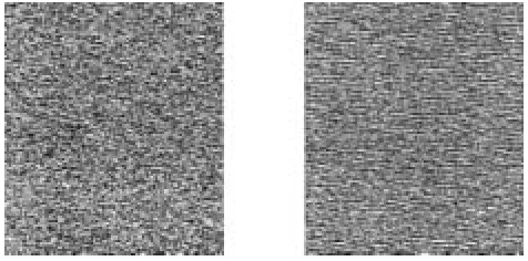
means neighbors of clique type (vertically, horizon-tally, or diagonally neighboring, etc.), is the standard devia-tion in the texture, and the are independent standard Gaussian errors. Condition imposes the causality. Fig. 1 shows a realization of a causal AR process with the second-order neigh-borhood system and a strong horizontal correlation, along with the Gaussian Markov random field with the same parameters for comparison. We see that the two are similar, but the MRF has a better defined texture. Simulations with other parameter values have supported this observation.
Fig. 1. Realization of a causal Gaussian AR process on the left, with a realization of the Gaussian Markov random field having the same parameters on the right.
MCMC. Under a first-order Potts model for , the log full con-ditionals are, up to an additive constant
(8)
where if , and is 0 otherwise, is the number of
different clique types in the neighborhood system, and the types and are the first-order doubleton cliques (horizon-tally and vertically neighboring pairs). Although causal models have computational advantages, the directionality implied in the definition means that they have less discriminating power than a Markov random field. However, in supervised segmentation, the model will still perform well in many situations, as we demon-strate later in Section IV. An early discussion of such causal models is in [4]. This model is an example of a Markov mesh model, further examples of which are in [5].
B. Model II: Ignore the Partition Function Term
Model II is defined by ignoring the partition function terms in (4). Doing this, we obtain the model of [6], which is used as a template model to divide an image into two regions. Again, a Markov structure on the posterior of is recovered. When a Potts model is assumed for and Gaussian conditional autoregressive (CAR) for the , that is, the follow the
non-causal AR model ,
where if , we obtain the following log full
conditional, up to an additive constant
(9)
We observe that this would be the posterior obtained from the double Markov random field, were the priors on the parame-ters to be proportional to the partition functions. However, there seems no argument, other than computational convenience, why one should specify such a prior.
C. Model III: Overlapping Window
Another possibility is to consider the grey levels to be com-posed of a set of overlapping square windows of size centered at , whose values are those of the corresponding window in . Within each window, the texture is assumed, and the windows are assumed independent given . This re-duces (4) to
(10)
where the partition function is that over . In the case of a CAR model with a toroidal boundary assumption, would be the normalizing constant of an -dimensional mul-tivariate normal, with mean and variance structure specified by ; see [7] for the form of the covariance matrix as a function of . Thus, is a function of the determinant of a
matrix, and readily computable for small , although the com-putational effort grows quickly with . In supervised segmen-tation, we need compute these only once (one for each texture), whereas in semi-unsupervised segmentation, they would have to be recomputed at each MCMC iteration. This model is used in [8]–[10], with windows of size 3 3; a similar model is pre-sented in [11].
For Gaussian CAR texture models and a Potts model for the labels, and with fixed boundary conditions, the log full condi-tionals of the posterior of are, up to an additive constant
Model III is susceptible to considerable boundary effects at the edges between different textures because a single texture model is assumed in each window. This effect increases with in-creasing window size. The minimum size of window that can be considered without losing textural information is one that con-tains the neighborhood of the central pixel. Model IV is then defined to be Model III but where the window size is the neigh-borhood of the central pixel. Thus
(12)
This model corresponds to using the pseudo-likelihood of the double Markov random field model for the posterior distribu-tion, as defined in [12]. The pseudo-likelihood has also been used in a Bayesian approach in [13]. The boundary effect still exists in that at the boundary this term is a function of some grey levels that are from another texture. Under Gaussian CAR texture models and a Potts model for the labels, the full condi-tionals of the posterior of are
(13)
E. Model V: Pseudo-Likelihood, but Ignore Grey Levels from a Different Texture
A modified version of (13) was used in [14], where only neighboring grey levels corresponding to pixels with the same label as pixel were included in the full conditional. Under Gaussian CAR textures and an Ising model prior for the labels, the full conditionals for the posterior of are
(14)
the sampling from the double MRF posterior. For the Gaussian MRF case, such conditional distributions on the are multi-variate Gaussian and can be calculated (see [15] for an efficient method). However, such an approach has its own problems. For texture classes with only a few pixels assigned, one is faced with simulating a realization of the texture across almost the entire image conditional on this small sample. Although not applied to image analysis, experience in [16] of simulation of Gaussian Markov random fields showed that convergence problems can easily arise. This would be particularly true in the semi-unsupervised case, where parameters from classes with only a few pixels assigned would not be well estimated. We do not pursue this idea further here.
G. Estimation of Model Parameters
In a Gibbs sampling scheme to simulate from (5), in a semi-unsupervised approach, we also require the full conditionals of all model parameters, which are a function of the partition func-tion. It is possible to approximate the partition function, but it is computationally expensive; see [17] for an example using the scheme of [18].
This approximation can only be practically evaluated for the texture parameters of Model I, where the dependence on the label parameter is from the partition function of the label model, and therefore, the partition function does not need to be re-eval-uated at each iteration of the sampler. In Models IV and V, we can make an approximation to the full conditional by restricting the dependence of the parameters to terms in (12). With uni-form prior distributions over some suitable range on all texture parameters, the full conditionals for are then proportional to the pseudo-likelihood function
(15)
In the case of Gaussian CAR parameters, the range of allowable values is determined in [19], and the full conditionals are given in [20, App. 2].
In all cases, where a Potts model is assumed for the labels, the full conditional of is not available. We either consider it fixed or sample from the pseudo-likelihood of the model; this latter case we call the adaptive algorithm.
the full conditionals [22]. Thus, this approach cannot be recom-mended if parameter estimates are the objective. However, we are interested merely in differentiating between classes and that
be calibrated to permit a reasonable segmentation.
H. Implementation Issues
To estimate the MPM segmentation using any of the models, one samples from the full conditional of the labels as specified; then, in the semi-unsupervised case, one also samples parame-ters; for Models IV and V, one can use (15). This is repeated until “convergence” occurs, whereupon samples are stored for each label. When “enough” have been collected, the most-often sam-pled label at each pixel after convergence is said to be the class at that point. The MAP segmentation is obtained using simu-lated annealing; therefore, it requires in addition a sequence of
temperatures decreasing to 0, and at the th
itera-tion of the MCMC sampler, labels are sampled from the dis-tribution proportional to
and parameters from that proportional to .
Once the temperature is near 0, the sampling stops, and the cur-rent segmentation is taken to be the MAP. Several temperature
sequences can be considered, such as geometric ( ,
for ) or logarithmic ( );
theo-retical discussion of the merits of these is found in [2].
We always initialize with a random segmentation, and on average, this seems to work well. One can, of course, start from an initial crude segmentation, but it is well documented that these MCMC approaches are liable to remain in local posterior maxima (see [23] for a simple example in the case of image restoration); therefore, the segmentation is sensitive to the starting conditions. For example, starting with a segmentation where all pixels are in one class, our experience is, even for the simple images to be analyzed in the next section, that the algorithm may only move slowly from this state. Other MCMC approaches to sampling labels, such as the Swendsen–Wang algorithm, can improve this situation [24].
[image:5.612.307.546.63.297.2]Another issue is the number of iterations. This depends on image size, complexity, and the number of classes, and there are clearly no absolute rules that one can follow. For MPM seg-mentation, we require that the MCMC has reached equilibrium before using the sampled labels to determine the MPM; mon-itoring or the number of pixels assigned to each class is an indicator of when the method has reached an equilibrium. In general, we then again run the algorithm for as many iterations as it took to reach equilibrium and use these to determine the MPM segmentation. For the MAP segmentation, too few iter-ations implies a quickly decreasing temperature and a risk of being caught in a local maximum far from the global. Our ex-perience is that 100 iterations is an absolute lower bound for either MAP or MPM, and for most images, many more will be needed. For example, for images of size 500 500, seg-mented into about five classes, 1000–2000 iterations are usu-ally required for MPM segmentation. We emphasize that these numbers are no substitute for monitoring and evaluation of the algorithm for each image that is segmented.
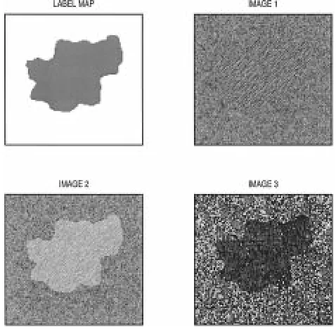
Fig. 2. Label map and the 3 textured images to be used in the simulation study.
IV. SIMULATIONEXPERIMENTS
In this section, we compare the five models with a simulation study. We assume second-order Gaussian CAR models for the textures and a Potts model for the labels, with the exception of Model I, where the causal AR model is assumed, that is, (8), (9), (11), (13), and (14) are the relevant full conditionals for . Three different 128 128 images are used, as displayed in Fig. 2. Each is composed of two textures according to the true label map in the figure. Images 1 and 2 are realizations of Gaussian CAR models, and image 3 is a composition of images of leaves and grass. In image 1, the mean and variance of both classes is the same, whereas in image 2, they are not.
Two sets of simulations are conducted, comprising a total of 49 experiments. The first set is supervised, with the main goal of comparing the performance of the five models. Within each set, there are various options we might select:
• model; • image;
• window size in the case of Model III; • whether to fix or sample it.
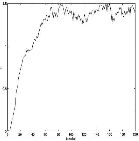
For the latter, we choose values of around and above the crit-ical value of 0.88 to compare with the sampled values, which were generally in the range 1.0–1.5 (see Fig. 3 for a typical trace of sampled values of ). The true texture parameter values are used for images 1 and 2 and the maximum likelihood estimates for image 3 (see [12]). A uniform prior for on the range (0, 4) is used, which gives support over critical temperature values.
Fig. 3. Sampled values of for semi-unsupervised segmentation of Image 1 using Model IV.
functions on the window has to be redone at each iteration. Model V then fails to give a good segmentation at all if one starts at an initially random configuration of labels because many sites would have few neighbors of the same label; therefore, the full conditional of the texture parameters contains no information from the data. In this set, therefore, we concentrate on the effect of sampling on the segmentation. Eight different experiments are run. Uniform priors are assumed for all CAR parameters: over [0, 255] for , [0, 255 ] for , and over the allowable range for the clique parameters.
For both supervised and semi-unsupervised experiments, Gibbs sampling was used, with an initial burn-in of 100 iterations, and the MPM taken to be the most observed label at each site on the next 100 iterations. This is a small number of iterations, but it is adequate for such small and simple images; see Fig. 3, which shows sampled values of for segmentation of image 1 using Model IV, which converges after about 80 iterations. Note that the value of is considerably over the “critical” temperature of the Ising model, at , supporting the observation that the pseudo-likelihood overes-timates . The adequacy of the number of iterations was also determined by pilot runs of 500 iterations. Each experiment consisted of 100 separate segmentation runs. Since the MPM is that segmentation that minimizes the expected number of misclassified labels, we adopt as our performance measure the number of misclassified labels in the MPM segmentation, compared with the true label map in Fig. 2.
A. Supervised Segmentation
Table I lists each of the 41 experiments conducted under su-pervised segmentation. In almost all comparable cases, the use of Model IV or V gives better results than for Models II or III. The performance of Model I can be good but is very sensitive to the choice of , and further, it performs very badly when is sampled. Between Models IV and V, no strong conclusions can
[image:6.612.363.495.102.495.2]TABLE II
MEDIAN ANDINTERQUARTILERANGE(INPARENTHESES)OF THEPERCENTAGE OFMISCLASSIFIEDPIXELSOVER100 RUNS OF THESEMI-UNSUPERVISED
[image:7.612.47.285.99.401.2]SEGMENTATIONEXPERIMENTSWITHMODELIV
Fig. 4. Results of Experiments 42 to 49. Boxplots of misclassified pixels under Model IV with Image 1 over 100 segmentations with (a) = 0:8, (b) = 1:0, (c) = 1:1, (d) = 1:3, (e) = 1:5, and (f) adaptive.
images 2 and 3 but worse in image 1. We believe that because the classes in images 2 and 3 are so distinct, Model V has the advan-tage over Model IV because it eliminates any boundary effects by excluding pixels in the other class from the full conditional. However, in image 1, the boundary effect is much less because the classes have the same mean and variance. In this case, what dominates is the greater uncertainty (in the sense that the full conditional probability of each class is nearer 0.5) with Model V than Model IV at boundaries because the full conditional is not based on the full neighborhood. We therefore conclude that Model V is preferable over Model IV when the classes have dis-tinct means but not when classes are close in mean.
There is also considerable difference in the variability in per-formance, as indicated by the interquartile range. This seems to be mainly an image effect, with the most challenging (image 1) showing the largest variability.
B. Semi-Unsupervised Segmentation
[image:7.612.310.544.325.558.2]Table II lists each of the eight experiments conducted under semi-unsupervised segmentation. For Image 1, the segmenta-tion algorithm with fixed is compared with the adaptive ver-sion, where the latter gives better results (experiments 42–47, see also Fig. 4). Each run took, on average, only 2% longer for the adaptive case than the fixed case. Therefore, we conclude that sampling improves the segmentation.
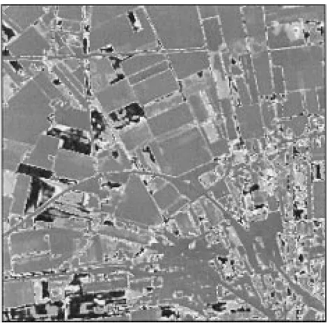
Fig. 5. Radar image of an agricultural region of Holland.
Fig. 6. MPM segmentation of the image in Fig. 5 into four classes.
When comparing the results of the adaptive segmentation al-gorithm on the three images (experiments 47–49), it can be seen that there is more variability in the results corresponding to the image composed by natural textures, whereas the best results are obtained with Image 2.
V. APPLICATION TO ASATELLITEIMAGE
Fig. 7. MPM segmentation of the image in Fig. 5 into five classes.
Fig. 8. Entropy of MPM segmentation of the image in Fig. 5 into four classes.
the results for an MPM segmentation into four classes. Fig. 7 then shows the MPM segmentation into five classes, based on the same number of iterations. We see that the classes assigned black and dark gray in Fig. 6 have remained but that the other two classes have been split and divided out very differently into three new classes in Fig. 7. The classification into five classes certainly appears less tidy, but it has distinguished a new class (assigned white) of lighter colored fields.
[image:8.612.302.553.61.312.2]Some of the additional analyses available, in the four-class case, from the MCMC are given in Figs. 8 and 9. Fig. 8 is the entropy in marginal posterior distribution of each label, that is
Fig. 9. Estimates of the posterior density of (top) the mean intensity for class 2, which is colored dark gray in Fig. 6, and (bottom) the percentage of pixels in class 2.
where is the proportion of times was sampled as class , with lighter colors indicating higher entropy. This gives a mea-sure of uncertainty in the class of each pixel, and we see that class 2 (colored dark gray in the segmentation) has the lowest uncertainty in general, and the highest uncertainty occurs at the borders between regions.
By looking at the relative proportion of values sampled, esti-mates of posterior distributions of parameters can be made. The top of Fig. 9 is an estimate of the posterior distribution of the mean of class 2. Similar plots can be made for all other model parameters, although we recall that the pseudo-likelihood may not be a good approximation for the posterior of correlation pa-rameters. Having recorded at each iteration the number of pixels in each class, we can construct the lower plot, which is an es-timate of the posterior distribution of the percentage of pixels that are in this class: something that might be of interest in ap-plications to land-use estimation.
VI. CONCLUDINGREMARKS
Any simulation study of the type we have described cannot hope to address all the interesting issues and must restrict itself in some way. In this study, we have concentrated on how the five methods perform on simple images and on the value of adapting using the pseudo-likelihood approximation. Other interesting issues that we have not addressed include MPM versus MAP segmentation, performance on larger images with more classes, the effect of assuming different order neighborhoods for labels and textures, and the performance of the MCMC method for the true double Markov random field model.
[image:8.612.48.285.317.549.2]is the only one that we have been able to implement satisfacto-rily. Where classes have distinct means, Model V may be better at the expense of greater computing time. We also conclude that in general, sampling of from the pseudo-likelihood improves the segmentation, in spite of the fact that it tends to be overesti-mated.
Some future developments of these techniques include fully unsupervised segmentation using Markov random field models, where is unknown. This is possible under the Bayesian ap-proach by MCMC if one uses reversible jump methods, but this is at the expense of considerable additional computational effort [25], [26]. The issue of what constitutes a reasonable prior for , or what loss function is appropriate for such segmentation, still needs to be addressed; this latter issue clearly depends on the ob-jective of the segmentation. Indeed, development of techniques that allow a wider range of loss functions to be used, other than 0–1 and number of misclassified pixels, would allow the method to be specialized for particular applications. Some discussion of possible alternative loss functions in image analysis more gen-erally are given in [27] and [28]. Such developments will add further computational costs to the approach, but we emphasize that the power of the MCMC approach is not in its speed but in the additional information on uncertainties in the segmentation that can be obtained.
ACKNOWLEDGMENT
The authors would like to thank the Centre National d’Etudes Spatiales, France, for the satellite image.
REFERENCES
[1] J. Zhang, J. W. Modestino, and D. A. Langan, “Maximum likelihood estimation for unsupervised model-based image segmentation,” IEEE Trans. Image Processing, vol. 3, pp. 404–419, July 1994.
[2] S. Geman and D. Geman, “Stochastic relaxation, Gibbs distributions and the Bayesian restoration of images,” IEEE Trans. Pattern Anal. Machine Intell., vol. PAMI-6, pp. 721–741, 1984.
[3] M. L. Comer and E. J. Delp, “Segmentation of textured images using a multiresolution Gaussian autoregressive model,” IEEE Trans. Image Processing, vol. 8, pp. 408–420, Mar. 1999.
[4] L. Baum, T. Petire, G. Souiles, and N. Weiss, “A maximization technique occurring in the statistical analysis of probabilistic functions of Markov chains,” Ann. Math. Statist., vol. 41, no. 1, pp. 164–171, 1970. [5] M. Titterington, A. J. Gray, and J. W. Kay, “An empirical study of the
simulation of various models used for images,” IEEE Trans. Pattern Anal. Machine Intell., vol. 16, pp. 507–513, Apr. 1994.
[6] D. B. Phillips and A. F. M. Smith, “Dynamic image analysis using Bayesian shape and texture models,” Adv. Appl. Statist. (supplement to J. Appl. Statist.), vol. 20, no. 5/6, pp. 299–322, 1993.
[7] R. L. Kashyap and R. Chellappa, “Choice of neighbors in spatial-inter-action models of images,” IEEE Trans. Inform. Theory, vol. IT-29, pp. 60–72, Feb. 1983.
[8] H. Derin and W. S. Cole, “Segmentation of textured images using Gibbs random fields,” Comput. Graph. Image Process., vol. 35, pp. 72–98, 1986.
[9] H. Derin and H. Elliott, “Modeling and segmentation of noisy and tex-tured images using random fields,” IEEE Trans. Pattern Anal. Machine Intell., vol. PAMI-9, pp. 39–55, Jan. 1987.
[10] B. S. Manjunath, T. Simchony, and R. Chellappa, “Stochastic and de-terministic networks for texture segmentation,” IEEE Trans. Acoust., Speech, Signal Processing, vol. 38, pp. 1039–1049, June 1990. [11] S. Geman and C. Graffigne, “Markov random field models and their
application to computer video,” in Proc. Int. Congr. Math., M. Gleason, Ed. Providence, RI: Amer. Math. Soc., 1987, pp. 1496–1517.
[12] J. Besag, “Spatial interaction and the statistical analysis of lattice sys-tems (with discussion),” J. R. Statist. Soc. B, vol. 36, pp. 192–236, 1974. [13] J. Heikkinen and H. Högmander, “Fully Bayesian approach to image restoration with an application in biogeography,” Appl. Stat., vol. 43, no. 4, pp. 569–583, 1994.
[14] F. S. Cohen and D. V. Cooper, “Simple parallel hierarchical and relax-ation algorithms for segmenting noncausal Markovian random fields,” IEEE Trans. Pattern Anal. Machine Intell., vol. PAMI-9, pp. 195–219, Feb. 1987.
[15] H. Rue, “Fast sampling of Gaussian Markov random fields,” J. R. Statist. Soc. Ser. B, vol. 63, no. 2, pp. 325–338, 2001.
[16] L. Knorr-Held and H. Rue. (2001) On block updating in Markov random field models for disease mapping. Tech. Rep.. [Online]. Available: www.stat.uni-muenchen.de/~leo/publikationen.html.
[17] I. S. Weir, “Fully Bayesian reconstructions from single-photon emission computed tomography data,” J. Amer. Statist. Assoc., vol. 92, no. 437, pp. 49–60, 1997.
[18] C. J. Geyer and E. A. Thompson, “Constrained Monte Carlo maximum likelihood for dependent data (with discussion),” J. R. Statist. Soc. B, vol. 54, pp. 657–699, 1992.
[19] S. Lakshmanan and H. Derin, “Valid parameter space for 2-D Gaussian Markov random fields,” IEEE Trans. Inform. Theory, vol. 39, pp. 703–709, Apr. 1993.
[20] D. E. Melas, “A Bayesian approach to the segmentation of textured im-ages,” Ph.D. dissertation, Dept. Statist., Univ. Dublin, Trinity College, Dublin, Ireland, 1999.
[21] A. M. Higdon, “Spatial applications of Markov chain Monte Carlo for Bayesian inference,” Ph.D. dissertation, Dept. Statist., Univ. Washington, Seattle, 1994.
[22] C. J. Geyer, “Markov chain Monte Carlo maximum likelihood,” in Proc. 23rd Symp. Interface, 1991, pp. 156–163.
[23] D. M. Greig, B. T. Porteus, and A. H. Seheult, “Exact maximum a pos-teriori estimation for binary images,” J. R. Statist. Soc. B, vol. 51, pp. 271–279, 1989.
[24] R. H. Swendsen and J.-S. Wang, “Nonuniversal critical dynamics in Monte Carlo simulations,” Phys. Rev. Lett., vol. 58, pp. 86–88, 1987. [25] Z. Kato, “Bayesian color image segmentation using reversible jump
Markov chain Monte Carlo,” Eur. Res. Consort. Inform. Math., Res. Rep. 01/99-R055, 1999.
[26] S. A. Barker and P. J. W. Rayner, “Unsupervised image segmentation using Markov random field models,” Pattern Recogn., vol. 33, pp. 587–602, 2000.
[27] H. Rue, “New loss functions in Bayesian imaging,” J. Amer. Statist. Assoc., vol. 90, pp. 900–908, 1995.
[28] H. Rue and A. Frigessi, “Bayesian image classification using Baddeley’s delta loss,” J. Comput. Graphic. Stat., vol. 6, no. 1, pp. 55–73, 1997.
Dina E. Melas received the Ph.D. degree from the
Department of Statistics, Trinity College, Dublin, Ire-land.
She is currently with Interoperability Systems In-ternational, Athens, Greece.
Simon P. Wilson received the Ph.D. degree in
sto-chastic modeling from the George Washington Uni-versity, Washington, DC.