A correction for sample overlap in genome wide association studies in a polygenic pleiotropy informed framework

M E T H O D O L O G Y A R T I C L E

Open Access

A correction for sample overlap in

genome-wide association studies in a

polygenic pleiotropy-informed framework

Marissa LeBlanc

, Verena Zuber

, Wesley K. Thompson

, Ole A. Andreassen

, Schizophrenia and

Bipolar Disorder Working Groups of the Psychiatric Genomics Consortium, Arnoldo Frigessi

and Bettina Kulle Andreassen

Abstract

Background: There is considerable evidence that many complex traits have a partially shared genetic basis, termed pleiotropy. It is therefore useful to consider integrating genome-wide association study (GWAS) data across several traits, usually at the summary statistic level. A major practical challenge arises when these GWAS have overlapping subjects. This is particularly an issue when estimating pleiotropy using methods that condition the significance of one trait on the signficance of a second, such as the covariate-modulated false discovery rate (cmfdr).

Results: We propose a method for correcting for sample overlap at the summary statistic level. We quantify the expected amount of spurious correlation between the summary statistics from two GWAS due to sample overlap, and use this estimated correlation in a simple linear correction that adjusts the joint distribution of test statistics from the two GWAS. The correction is appropriate for GWAS with case-control or quantitative outcomes. Our simulations and data example show that without correcting for sample overlap, the cmfdr is not properly controlled, leading to an excessive number of false discoveries and an excessive false discovery proportion. Our correction for sample overlap is effective in that it restores proper control of the false discovery rate, at very little loss in power.

Conclusions: With our proposed correction, it is possible to integrate GWAS summary statistics with overlapping samples in a statistical framework that is dependent on the joint distribution of the two GWAS.

Keywords: Data integration, Meta-analysis with shared subjects, Covariate-modulated false discovery rate, Cross-phenotype association

Background

The past decade of genomic research has been shaped by the advent of low-cost, high throughput technology, enabling the examination of a large number of genetic variants, i.e. single nucleotide polymorphisms (SNPs), via the genome-wide association study (GWAS). The success of the GWAS approach has been limited however because SNPs identified by GWAS only capture a small fraction of the total heritability for any given complex trait. There is ongoing debate on how to detect this so-called ‘missing

*Correspondence:[email protected]

†_{Marissa LeBlanc and Verena Zuber contributed equally to this work.} 1_{Oslo Centre for Biostatistics and Epidemiology, Oslo University Hospital, Oslo} universitetssykehus HF, Sogn Arena, PB 4950 Nydalen, 0424 Oslo, Norway Full list of author information is available at the end of the article

heritability’ [1, 2], including ideas based on integrating GWAS data across two or more traits which may share a polygenic signal (e.g. [3]). A shared polygenic signal may exist for traits with strong diagnostic overlap and this has motivated the formation of cross-trait GWAS consortia such as the Psychiatric Genetics Consortium including five psychiatric diseases, and the International Cancer Genome Consortium that aims at finding oncogenes that might drive cancer growth in different sites. Seemingly unrelated phenotypes may also have a shared polygenic signal if they partially share a common genetic basis, termed pleiotropy [4]. Pleiotropic effects have been statis-tically detected in cross-trait analysis of GWAS, including schizophrenia and blood lipids [3], prostate cancer and blood lipids [5], and psychiatric disorders [6].

A major statistical challenge encountered when integrating GWAS data across traits is the widespread re-use of subjects between GWA studies, leading to non-independent data sets. Power has been maximized by increasing sample sizes, often in the hundreds of thousands, via large meta-analysis conducted by world-wide consortia for complex traits such as coronary artery disease (CAD) [7], height [8] and blood pressure [9]. Sec-ond, phenotype definitions have become more specific and have moved towards endophenotypes (e.g. blood lipids [10]), which are often measured on the same set of individuals. This, together with the epidemiological overlap of many common diseases, has led to the re-use of subjects from one GWAS to another. For example, control samples have been re-used for several different case definitions, often by design. The Wellcome Trust Case Control Consortium (WTCCC) [11] is one such consortium adopting this strategy. As another example, cases for one trait have been included in quantitative trait studies (e.g. CAD [7] and blood lipids [10] and height [8]). Addressing subject overlap is complicated by that fact that GWAS data is most often made available in form of summary statistics, i.e data overnsamples is condensed into one summary statistic per SNP. GWAS summary statistics from studies with overlapping subjects cannot be made independent by removing these subjects. Aside from the issue of sample overlap, working on the summary statistics level has many advantages. When a sufficient statistic is used this summary statistic contains all the information necessary for further inference. Also, it is computationally efficient to work with summary statis-tics simply because of the much smaller size compared to the genotype data. This is especially relevant for the integration of several genomic data sets. Importantly, in contrast to genotype data, summary statistics cannot be used to uniquely identify individuals. This allows easier distribution and storage. As a consequence there are sev-eral consortia, such as the DIAGRAM Consortium for type 2 diabetes and the Global Blood Lipids Consortium, that have summary statistics covering the whole genome for free download on their homepage.

Lin and Sullivan [12] were the first to address the methodological challenge of integrating GWAS with over-lapping subjects. Their contribution focused on integrat-ing case-control GWAS usintegrat-ing a meta-analysis framework. They do not provide a framework for integrating GWAS coming from different types of outcome variables (e.g. a case-control study and a quantitative trait study), nor do they provide a solution that applies in general to different statistical methodology. Han et al. [13] extend the Lin and Sullivan approach for cases and controls to random effects meta-analysis setting using a decoupling approach.

Two other approaches for meta-analysis of multiple traits while accounting for sample overlap are presented

by [14,15]. While these two approaches account for sam-ple overlap in performing the meta-analysis, [16] intro-duce a test statistic based on a similar derivation as Lin and Sullivan that allows to test for overlapping samples or relatives when performing quality control of summary level data.

There is growing interest in statistical methods that uti-lize the joint bivariate distribution of GWAS summary statistics for two traits because, in the presence of a shared polygenic signal, these methods may provide more power than traditional GWAS methodology. One such method is the covariate-modulated local false discovery rate (cmfdr) proposed by Ferkingstad et al. [17] and recently revisited and extended [18] where the fdr for the first study depends on a covariate, for example the GWAS summary statistics for a second pleiotropic trait.

Similarly, the tail-area based conditional false discovery rate [3] needs the joint distribution of two sets of GWAS summary statistics to identify SNPs with cross-phenotype associations. These methods may be seriously impacted by the spurious correlation due to overlap, but cannot be corrected on a SNP-by-SNP basis. Liley and Wallace [19] extend the conditional false discovery rate [3] to studies with overlapping controls. Their extension is specific to case-control studies and does not apply to the cmfdr or any other bivariate method.

The aims of this paper are threefold. First, we want to show the impact of overlap in samples on integrated analy-ses of genetic studies. We show that it can induce spurious correlation between the studies and thus seriously con-found conclusions. Second, we expand on the work of Lin and Sullivan [12] and quantify the spurious cross-trait cor-relation due to overlap for both case-control studies and studies with quantitative traits. And third, we propose a correction based on a decorrelation transformation that adjusts the joint distribution of two GWAS and allows for the use of the corrected summary statistics in down-stream analysis such as cmfdr. We demonstrate the impact of overlap in samples and the success of our proposed cor-rection on synthetic and GWAS data from the Psychiatric Genetics Consortium (PGC).

Results

The impact of overlap in samples on the joint analysis of two genomic data sets

and probability of success equal to the MAF. Each study has a continuous outcome that only depends on the error term (normal with mean 0 and standard deviation of 1). Study 1 and study 2 have nC = 5, 000 shared subjects andnA= nB= 7, 500 unique subjects respectively. Thus the total sample size per study isn1 = n2 = 12, 500. We

then conduct a standard GWAS analysis (univariate linear regression, one SNP at a time) separately in study 1 and study 2.

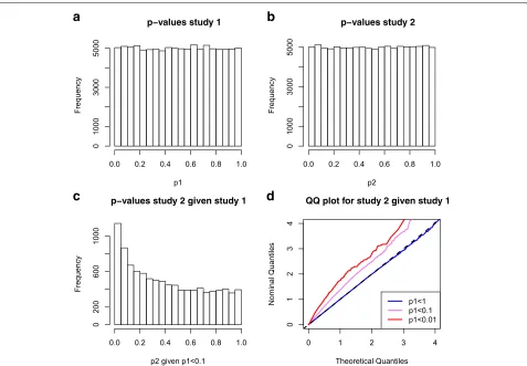
Figure 1a and b show that p-values for study 1 and for study 2 respectively follow a uniform distribution as expected. Assume we are interested in selecting the SNPs in study 2 on the basis of their significance in study 1. Figure 1c shows the p-values of study 2 for which the p-values in study 1 are smaller than 0.1. Finally, Fig. 1d displays a stratified Q-Q plot that plots the observed quantiles of the p-values of study 2 against the quantiles assumed under the null distribu-tion. The strata are defined with respect to thep-values in study 1. These stratified Q-Q plots offer an intuitive way

of visualizing dependencies betweenp-values of two dif-ferent genetic studies. Despite being generated without any genetic effects, we observe that the conditional dis-tributions of p-values from study 2 given p-values in study 1 show strong enrichment for smallp-values with respect to the second conditional phenotype. If we were unaware that these simulations were conducted under the null hypothesis, this leftward deflection of the stratified Q-Q plot could be falsely interpreted as shared polygenic pleiotropic signal. Clearly, in case of overlapping samples, pleiotropic effects would be confounded with the spurious effects due to sample overlap.

Estimating the correlation of two test statistics due to overlap in samples

Details of this estimation are given in the “Methods” section. Consider two studies,k = 1, 2, both with con-tinuous outcomes,yki,i = 1,. . .,nk. Assume some sam-ples are shared, so that we can split the set of samsam-ples

{1,. . .,nk} into two sets SC = {1,. . .,nc} and SA =

a

c

d

b

Fig. 1Simulated GWAS pairs with overlapping samples. Data was simulated for two quantitative trait GWAS with no genetic effects but overlap in

samples (each withn=12, 500 including 5000 overlapping samples).d=100, 000 SNPs were simulated under the null model (phenotype is

simulated independent from genotype). Panela: thep-value distribution for trait 1; Panelb: thep-value distribution for trait 2; Panelc: Thep-value

distribution for trait 2 given that thep-value in study 1 was less than 0.1; Paneld: quantile-quantile plot for thep-values in study 2, stratified by the

{nc+1,. . .,n1}for study 1 and similarily for study 2 with

SB = {nc+ 1,. . .,n2}. SC are the shared samples and SAandSBare the samples unique to study 1 and study 2 respectively. The full set for study 1 isS1 = SC ∪SAand for study 2 isS2=SC∪SB. Denote withXkigthe random genotypes for SNPg in sampleiin studyk,g = 1, 2, ..,d, wheredis typically some large number (≈106). Simlarly, denote withXkjgthe random genotypes in samplej.Then, cor(X1ig,X2jg)=1 ifi∈SCfor all SNPsgand we assume cor(X1ig,X2jg)=0 ifi∈SAandj∈SBfor allg.

Consider two regression models, one for each study for one SNP g at a time, Y1i = α1g + β1gX1ig + 1ig and Y2j = α2g+β2gX2jg+2jgwherei = 1, ..,n1,j= 1, ..,n2,

and we assume all errors to be independent from each other and with zero mean. Under the null model (β_kg=0)

∀k,g, ifSC was an empty set (i.e. no shared subjects), then corβˆ1g,βˆ2g

= 0. But because of the shared samples SC, ρ = cor

ˆ β1g,βˆ2g

= 0, the overlap between sam-ples introduces a correlation of the regression parameters which is only due to the overlap. Note, when analyzing study 1 and study 2 separately the analysis is unbiased; the bias due to overlap is only introduced in a joint analysis whereρ=0 is neglected, as illustrated in Fig.1.

Building on the work of Lin and Sullivan [12], we esti-mate the correlationρdue to overlap in samples under the null model (βkg =0)∀k,g, using the correlation between the maximum likelihood (ML) estimates for the regression coefficients for SNPgdenoted byβˆkg. The ML estimates are asymptotically Gaussian distributed with mean equal to the true coefficients β_kg and variance equal to the inverse Fisher information.

We are also interested in combined analysis of GWAS summary statistics from other study designs, including those analyzed in a case-control study. Therefore, in the following we estimate ρ for three possible scenar-ios with (Y1 and Y2 both quantitative; Y1 quantitative

and Y2 binary; Y1 and Y2 both binary, where Yk =

{Yk1,Yk2,. . .,Yknk} fork = 1, 2). The ML-based

deriva-tions (see “Methods” section) result in the following esti-mated correlation due to sample overlap for each of the three possible study design pairings:

1 Quantitative phenotype in both study 1 and study 2. For each SNPg,

cor(βˆ1g,βˆ2g)≈ nc

√

n1·n2cor(

Y1,Y2) (1)

wherencis the number of overlapping samples in study 1 and 2,n1is the sample size of study 1, andn2

the sample size of study 2, respectively. Note that under the null hypothesis of no SNP effect, this correlation does not depend on the MAF and is the same for every SNP. In this case theg subscript can

be dropped and corβˆ1g,βˆ2g

can instead be written

as corβˆ1,βˆ2

, and this simplified notation is used from this point on.

2 Binary phenotype in study 1 and binary phenotype in study 2

corβˆ1,βˆ2

≈√_n1

1√n2×

nc0

exp{α1+α2} +

nc1

√

exp{α1+α2}

(2)

whereexp{α1+α2} ≈n11n21/n10n20[12] and where

we denote the number of cases in study 1 and 2 as

n11andn21respectively, similarlyn10andn20for the

number of controls in study 1 and 2 respectively, and denote the overlap in controls bync0and in cases by

nc1.

3 Quantitative phenotype in study 1 and binary phenotype in study 2

cor

ˆ β1,βˆ2

≈ nc

√

n1·n2

corpb(Y1,Y2) (3)

where cor_pb(Y1,Y2)equals the point-biserial

correlation coefficient.

Note that the estimatescorβˆ1,βˆ2

in Eqs.1to3only estimate the spurious correlation due to sample overlap. This estimate differs from the total correlation between the observed test statistics which captures both the true correlation based on genetic architecture and the spurious correlation induced by sample overlap.

Decorrelation using the correlation due to overlap

In this paper we propose a decorrelation step to adjust the joint distribution of the summary statistics from two GWAS having overlapping subjects. Construct a matrix z consisting of two rows anddcolumns equal to the num-ber of SNPs common to both studies, including the vector of summary statistics (z-scores) for the first study,z1, in

the first row and the vector of z-scores for the second study,z2, in the second row. The decorrelation transform

is defined as

zde-corr=C−1/2z (4)

where C is the 2×2 matrix with ones on its diagonal the calculated correlation due to overlap on its off-diagonal.

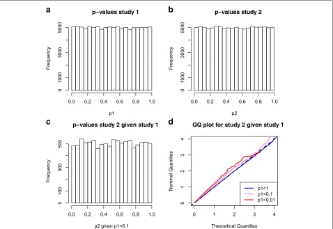
In Fig.2we use the simulated data introduced in Fig.1

a

b

c

d

Fig. 2Simulated GWAS pairs with overlapping samples, after correction for sample overlap using the decor relation transform. Data before

correction is presented in Fig.1. Data was simulated for two quantitative trait GWAS with no genetic effects but overlap in samples ((each with

n=12, 500 including 5,000 overlapping samples).d=100, 000 SNPs were simulated under the null model (phenotype is simulated independent

from genotype). The decor relation transformation proposed here was applied to the simulated summary statistics. Panela: thep-value distribution

for trait 1; Panelb: thep-value distribution for trait 2; Panelc: Thep-value distribution for trait 2 given that thep-value in study 1 was less than 0.1;

Paneld: quantile-quantile plot for thep-values in study 2, stratified by thep-value in study 1

Performance of proposed decorrelation step in a covariate-modulated false discovery rate framework

We tested the performance of our proposed correction for sample overlap in a covariate-modulated fdr (cmfdr) [18] framework using a two-pronged approach. First, we quan-tified the impact of sample overlap on the actual false dis-covery proportion under different pleiotropic simulation scenarios and with different amounts of sample overlap. Second, we used individual-level (genotype-phenotype) data from the Psychiatric Genetics Consortium (PGC), which employed a shared control design for schizophre-nia and bipolar disorder, to test our correction in a real data setting. Since we had access to the individual-level data, we were able to conduct a series of GWAS manipu-lating the extent of overlapping controls and compare the number of cmfdr-based “discoveries” to equally-powered non-overlapping control sets.

Simulated data

We simulated bivariate GWAS data under six different simulation scenarios: first under the null model, where genotype is independent from phenotype and then under five different pleiotropic scenarios:

1 Null model, no effect 2 Positive pleiotropy A 3 Positive pleiotropy B 4 Positive pleiotropy C

5 Positive pleiotropy plus univariate effects 6 Positive and antagonistic pleiotropy,

where positive pleiotropy A, B and C differ in the extent of polygenic structure.

then again with sample overlap. For each study pair, we calculated the cmfdr for the first GWAS using the sum-mary statistics from the second GWAS as a covariate. We did this both with and without our proposed correc-tion for sample overlap and compared the false discovery proportion (FDP), i.e. the number of false discoveries divided by the total number of discoveries, before and after correction and to the non-overlapping GWAS.

Simulation results The main purpose of the simulation was to test the performance of our correction for sam-ple overlap in a cmfdr framework with known null and non-null SNPS under different pleiotropic and polygenic scenarios and with different amounts of sample overlap.

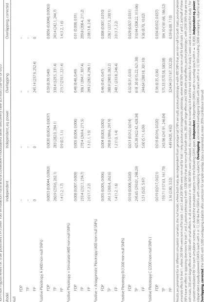
Table 1 reports the mean false discovery proportion (FDP), mean number of falsely rejected null hypotheses (i.e. false positives (FP)) and mean number of correctly rejected non-null hypotheses, (i.e. true positives (TP)) under different simulation scenarios withd = 100, 000 SNPs over independent 100 simulations based on a cmfdr cutoff of 0.05 and using the summary statistics from study 2 as a covariate for study 1. This is reported for all six sim-ulation scenarios. The null model simsim-ulation shows that, in the absence of any true genetic association and with non-overlapping samples, no SNPs reach the cmfdr cut-off of 0.05. In contrast, when samples overlap, a mean of 245 SNPs are below the cutoff, and thus are false positives. After applying our proposed correction to the GWAS with overlapping samples, all cmfdr values are again above the significance cutoff and no SNPs are deemed significant. For the simulation scenarios involving pleiotropic effects, 400 of the 100,000 SNPs were non-null except for positive pleiotropy B and C where 1200 and 2200 were non-null respectively. For all pleiotropic scenarios, the FDP for the analysis using the non-overlapping studies shows that the fdr level is conservatively held, while the FDP for the over-lapping set, greatly exceeds the desired level of fdr control. After correction the overlapping studies using the pro-posed decorrelation step, the fdr control is comparable to the non-overlapping, independent studies.

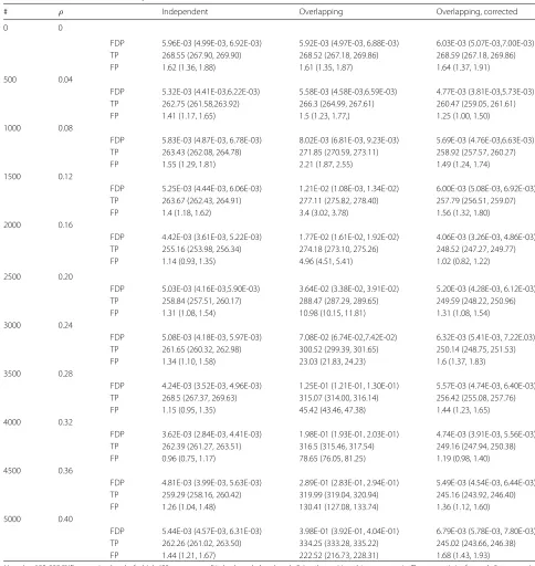
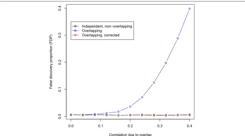
We performed an extended simulation using the “posi-tive pleiotropy A” scenario, where we varied the amount of sample overlap. Table2and Fig.3give the FDP, TP and FP and clearly show that the impact of sample overlap is non-linear. The FDP increases at an increasing rate as the number of overlapping samples increases. After applying our correction for sample overlap to the overlapping stud-ies, the fdr control is comparable to the non-overlapping, independent studies for all levels of sample overlap. The correction results in a small loss in power (TP), and this loss in power is more severe as the overlap increases.

In practice it may be difficult to calculate the exact overlap in samples or obtain an accurate estimate of Cor(Y1,Y2)for continuous traits. We therefore tested the

robustness of our proposed correction to the correlation used in the decorrelation step (Eq.4). Using the positive pleiotropy A scenario, wherecorβˆ1,βˆ2

= 0.4, we var-ied the correlation value used in Eq.4from 0.3 to 0.5. We find that our proposed correction is robust the the corre-lation value used in the decorrecorre-lation step with fdr level being conservatively held in all cases (Table3).

Psychiatric Genetics Consortium (PGC) data with shared controls

We used the PGC data [21,22] to test the performance of our proposed correction for sample overlap in a real data setting, where we varied the amount of overlap in the control group between the schizophrenia and bipo-lar studies, corresponding to an expected correlation of

ρ=0, 0.09, 0.18, 0.27, 0.36, 0.45. Using this series of GWAS summary statistics for bipolar disorder and schizophre-nia, we calculated the cmfdr using the bipolar disor-der summary statistics as the covariate for schizophre-nia. The cmfdr calculations were done for both the raw data and also for the data after correction for sample overlap.

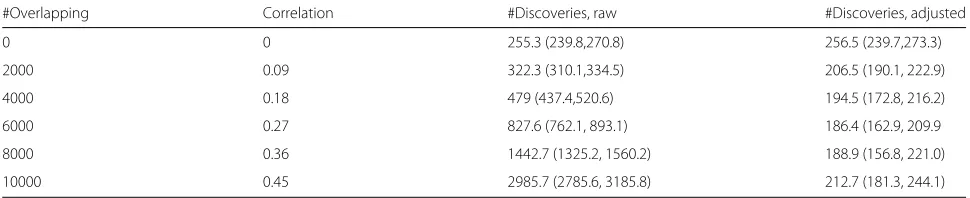
PGC results Which SNPs are null and which SNPs are non-null is unknown, so it is not possible to count the true and false positives. Instead, we can count the total number of SNPs below a given cmfdr threshold (TP+FP), and use the non-overlapping set as a reference point. In this case, we used a threshold of 0.05 and called all SNPs with a cmfdr below this threshold a discovery. Impor-tantly, the number of controls is held constant across the different amounts of sample overlap. This rules out any differences in (TP+FP) that may be expected to due differences in power. There were on average 255 discov-eries for the analysis with no overlapping controls and significantly more discoveries were made when samples overlapped, as is evident by the non-overlapping confi-dence intervals for the no overlapping controls scenario versus all overlapping scenarios (Table4). After correction for sample overlap, the number of discoveries returned to a more comparable level, usually falling just below the number of discoveries made in the non-overlapping analysis.

Discussion

Table 2Mean false discovery proportion (FDP), mean number of falsely rejected null hypotheses out of 99,600, i.e. false positives (FP) and mean number of correctly rejected non-null hypotheses out of 400 s, i.e. true positives (TP) over 100 simulation runs and a covariate-modulated false discovery rate (cmfdr) cut-off of 0.05

# _ρ Independent Overlapping Overlapping, corrected

0 0

FDP 5.96E-03 (4.99E-03, 6.92E-03) 5.92E-03 (4.97E-03, 6.88E-03) 6.03E-03 (5.07E-03,7.00E-03)

TP 268.55 (267.90, 269.90) 268.52 (267.18, 269.86) 268.59 (267.18, 269.86)

FP 1.62 (1.36, 1.88) 1.61 (1.35, 1.87) 1.64 (1.37, 1.91)

500 0.04

FDP 5.32E-03 (4.41E-03,6.22E-03) 5.58E-03 (4.58E-03,6.59E-03) 4.77E-03 (3.81E-03,5.73E-03)

TP 262.75 (261.58,263.92) 266.3 (264.99, 267.61) 260.47 (259.05, 261.61)

FP 1.41 (1.17, 1.65) 1.5 (1.23, 1.77,) 1.25 (1.00, 1.50)

1000 0.08

FDP 5.83E-03 (4.87E-03, 6.78E-03) 8.02E-03 (6.81E-03, 9.23E-03) 5.69E-03 (4.76E-03,6.63E-03)

TP 263.43 (262.08, 264.78) 271.85 (270.59, 273.11) 258.92 (257.57, 260.27)

FP 1.55 (1.29, 1.81) 2.21 (1.87, 2.55) 1.49 (1.24, 1.74)

1500 0.12

FDP 5.25E-03 (4.44E-03, 6.06E-03) 1.21E-02 (1.08E-03, 1.34E-02) 6.00E-03 (5.08E-03, 6.92E-03)

TP 263.67 (262.43, 264.91) 277.11 (275.82, 278.40) 257.79 (256.51, 259.07)

FP 1.4 (1.18, 1.62) 3.4 (3.02, 3.78) 1.56 (1.32, 1.80)

2000 0.16

FDP 4.42E-03 (3.61E-03, 5.22E-03) 1.77E-02 (1.61E-02, 1.92E-02) 4.06E-03 (3.26E-03, 4.86E-03)

TP 255.16 (253.98, 256.34) 274.18 (273.10, 275.26) 248.52 (247.27, 249.77)

FP 1.14 (0.93, 1.35) 4.96 (4.51, 5.41) 1.02 (0.82, 1.22)

2500 0.20

FDP 5.03E-03 (4.16E-03,5.90E-03) 3.64E-02 (3.38E-02, 3.91E-02) 5.20E-03 (4.28E-03, 6.12E-03)

TP 258.84 (257.51, 260.17) 288.47 (287.29, 289.65) 249.59 (248.22, 250.96)

FP 1.31 (1.08, 1.54) 10.98 (10.15, 11.81) 1.31 (1.08, 1.54)

3000 0.24

FDP 5.08E-03 (4.18E-03, 5.97E-03) 7.08E-02 (6.74E-02,7.42E-02) 6.32E-03 (5.41E-03, 7.22E.03)

TP 261.65 (260.32, 262.98) 300.52 (299.39, 301.65) 250.14 (248.75, 251.53)

FP 1.34 (1.10, 1.58) 23.03 (21.83, 24.23) 1.6 (1.37, 1.83)

3500 0.28

FDP 4.24E-03 (3.52E-03, 4.96E-03) 1.25E-01 (1.21E-01, 1.30E-01) 5.57E-03 (4.74E-03, 6.40E-03)

TP 268.5 (267.37, 269.63) 315.07 (314.00, 316.14) 256.42 (255.08, 257.76)

FP 1.15 (0.95, 1.35) 45.42 (43.46, 47.38) 1.44 (1.23, 1.65)

4000 0.32

FDP 3.62E-03 (2.84E-03, 4.41E-03) 1.98E-01 (1.93E-01, 2.03E-01) 4.74E-03 (3.91E-03, 5.56E-03)

TP 262.39 (261.27, 263.51) 316.5 (315.46, 317.54) 249.16 (247.94, 250.38)

FP 0.96 (0.75, 1.17) 78.65 (76.05, 81.25) 1.19 (0.98, 1.40)

4500 0.36

FDP 4.81E-03 (3.99E-03, 5.63E-03) 2.89E-01 (2.83E-01, 2.94E-01) 5.49E-03 (4.54E-03, 6.44E-03)

TP 259.29 (258.16, 260.42) 319.99 (319.04, 320.94) 245.16 (243.92, 246.40)

FP 1.26 (1.04, 1.48) 130.41 (127.08, 133.74) 1.36 (1.12, 1.60)

5000 0.40

FDP 5.44E-03 (4.57E-03, 6.31E-03) 3.98E-01 (3.92E-01, 4.04E-01) 6.79E-03 (5.78E-03, 7.80E-03)

TP 262.26 (261.02, 263.50) 334.25 (333.28, 335.22) 245.02 (243.66, 246.38)

FP 1.44 (1.21, 1.67) 222.52 (216.73, 228.31) 1.68 (1.43, 1.93)

Hered=100, 000 SNPs were simulated, of which 400 were non-null in both study 1 and study 2, i.e., the positive pleiotropy senario. The test statistics for study 2 were used as a covariate for study 1 for the covariate-modulated fdr. For each simulation, we divided the simulated subjects into the following GWAS pairs:Independent, independent GWASs with no overlap (each withn=10, 000),Overlapping, uncorrected, overlapping GWAS with (each with including between 0 and 5000 overlapping subjects) and

Overlapping, corrected, the GWAS with overlapping subjects after correction for sample overlap. Data is presented as mean (95% confidence interval) #, number overlapping.ρ, correlation due to overlap

genetic architecture models, we have quantified the mag-nitude of the effect of sample overlap on the covariate-modulated fdr and have shown that sample overlap can

Fig. 3Mean false discovery proportion (FDP) versus the correlation due to sample overlap over 100 simulation runs and a covariate-modulated false

discovery rate (cmfdr) cut-off of 0.05. Hered₌100, 000 SNPs were simulated, of which 400 were non-null in both study 1 and study 2, i.e., have

positive pleiotropic effects. The test statistics for study 2 were used as a covariate for study 1

comparable level to simulated scenarios with no sample overlap. Using data for bipolar disorder and schizophre-nia from the Psychiatric Genetics Consortium, we show that increasing numbers of shared controls result in an increased number of “discoveries”, but these so-called dis-coveries are most likely false positives and indicate a loss of proper control of the false discovery rate.

Statistical methods for integrating GWAS data at the summary statistic level are well established. Examples of such methods are Fisher’s method [23], inverse-variance meta-analysis [23], the conjunctional false discovery rate [3], the covariate-modulated fdr [18] and Mendelian ran-domization [24]. These methods universally assume inde-pendent samples. Violation of this assumption will result

in increased Type 1 error and biased effect estimates [24]. Lin and Sullivan [12] were the first to recognize this importance of the sample overlap problem in the context of cross-trait analysis of GWAS data. Their work is focused on correcting for sample overlap for case-control studies in the context of fixed-effects meta-analysis test statistics. Under the null hypothesis of no genetic effects, they derived the correlation between the maximum likeli-hood estimates for the logistic regression coefficients for a given SNP in study 1 and study 2 when there are par-tially overlapping subjects in case-control studies. Here we use the same approach to derive the correlation for a case-control GWAS paired with a quantitative trait GWAS, or for 2 quantitative trait GWASs. The spurious correlation

Table 3Robustness of the proposed correction

True correlation Plug-in correlation TP FP FDP

0.4 0.3 261.16 (260.27, 262.85) 2.42 (2.12, 2.71) 0.0091 (0.0080, 0.0102)

0.4 0.35 252.20 (250.92, 253.48) 1.56 (1.32, 1.80) 0.0061 (0.0052, 0.0070)

0.4 0.375 247.78 (246.79, 249.06) 1.48 (1.22, 1.73) 0.0059 (0.0049, 0.0069)

0.4 0.4 243.59 (242.31, 244.879) 1.40 (1.17, 1.63) 0.0057 (0.0048, 0.0066)

0.4 0.425 238.72 (237.42, 240.02) 1.60 (1.38, 1.82) 0.0066 (0.0057, 0.0075)

0.4 0.45 235.11 (233.88, 236.34) 1.96 (1.72, 2.20) 0.0082 (0.0072, 0.0092)

0.4 0.5 234.81 (233.57, 236.04) 1.96 (1.72, 2.20) 0.0082 (0.0072, 0.0092)

Table 4Psychiatric Genetics Consortium data, with varying amounts of overlapping controls

#Overlapping Correlation #Discoveries, raw #Discoveries, adjusted

0 0 255.3 (239.8,270.8) 256.5 (239.7,273.3)

2000 0.09 322.3 (310.1,334.5) 206.5 (190.1, 222.9)

4000 0.18 479 (437.4,520.6) 194.5 (172.8, 216.2)

6000 0.27 827.6 (762.1, 893.1) 186.4 (162.9, 209.9

8000 0.36 1442.7 (1325.2, 1560.2) 188.9 (156.8, 221.0)

10000 0.45 2985.7 (2785.6, 3185.8) 212.7 (181.3, 244.1)

The test statistics for bipolar disorder were used as a covariate for schizophrenia in the covariate-modulated fdr (cmfdr). SNPs having a cmfdr<0.05 were called as discoveries. Data is presented as mean (95% confidence interval)

due to sample overlap is derived under the null and quan-tifies the correlation which is solely induced by sample overlap and independent of any genetic effect. Others have recognized that the number of overlapping sam-ples is not always known and have proposed methods for estimating the correlation due to overlap using summary statistics alone [14,25]. These methods could be used for quantitative trait GWASs where in practice the correla-tion of the two phenotypes (Cor(Y1,Y2)) may be difficult

to estimate. Our simulations show that our proposed cor-rection is robust with respect to the assumed correlation due to overlap. Further, the impact ofCor(Y1,Y2)on the

correlation due to overlap increases as the extent of over-lap increases. In these cases it may be feasible to request an estimate ofCor(Y1,Y2)from the relevant GWAS

con-sortium. Regardless of which method is used to derive the correlation induced by sample overlap, here we propose a general framework to account for this spurious correlation in a simple and yet efficient preprocessing step. Spuri-ous correlation between test statistics can be introduced not only by sample overlap, but also by including rela-tives in both studies. This results in an effective number of overlapping samples a concept introduced in [16]. Our approach can be easily extended to account for the effec-tive number of overlapping samples in replacingncby the effective number of overlapping samples.

Conclusions

Our goal was to provide a more general solution to the problem of cross-trait integration of GWAS that could be applied to statistical methods depending on the joint dis-tribution of 2 GWASs. It is a practical approach in that it is easy to implement and results in transformed test statis-tics that can be used in different data integration methods. We show that in a cmfdr setting, our correction properly maintains fdr control.

Here we have contributed to the growing body of evi-dence showing that sample overlap needs to be taken into account when integrating data across different traits. We have shown that our flexible and adaptable adjustment for sample overlap works well as shown with both simulation and with real data in the context of the cmfdr.

Methods

Derivation of the estimates for correlation due to overlap

The correlation due to overlap in samples is derived from the correlation of the maximum likelihood (ML) estimates of the regression coefficients between two studies under the assumption of no genetic effect. We focus on one regression per SNP g and include the intercept and no other covariates. Focusing first on quantitative outcomes, consider two linear regressions, for one SNP g(we drop the indexg),Yk=αk+βkXk+k. We assume all errorsk to be independent from each other and with zero mean.

Lin and Sullivan [12] show that for two case con-trol studies the covariance between the ML esti-mates of the logistic regression coefficients from study 1 and 2 can be approximated as Cov

ˆ β1,βˆ2

≈

I₁−1(β1)Cov(U1(β1),U2(β2))I2−1(β2) whereUk andIk are the score function and Fisher’s information with respect to βk. We use the above to further define the following correlation:

Corβˆ1,βˆ2

≈I₁−1/2(β1)Cov(U1(β1),U2(β2))I2−1/2(β2).

(5)

It is now straightforward to expand this result to include quantitative trait studies using the ML estimates from linear regression.

For linear regression the score function with respect to

βkis given byU(βk)= _σ12 k

i∈Sk(yki−(αk+βkxki))xkiand

the Fisher information is given byI(βk)= _σ12 k

i∈Skxkixki.

Similarly for logistic regression the score func-tion with respect to βk is given by U(βk) =

i∈Sk

yki−₁₊exp_exp{α_{k_α+_k+βk_βx_kki_xki}_}

xki and the Fisher

informa-tion is given byI(βk)=

i∈Sk

exp{αk+βkxki}

(1+exp{αk+βkxki})2xkixki.

We make the following assumptions:

1 Ykis independent ofXk, that is we assume the null

model where there is no genetic effect in the data and βk=0for all SNPs,k=1, 2.

3 Construct a variableH defined asH=EXkX_kT .

We can estimateH under the null hypothesis and the following three estimates ofH are approximately equaln−₁1_i∈S1x1ix1i≈n−21

i∈S2x2ix2i≈n

−1

C

i∈SCx1ix2i.

In case-control studies we assume y1i = y2i for i ∈ SC (in other words cases in study 1 are cases in study 2). Thus Cor(Y1,Y2) = 1 for the

over-lapping samples in case-control studies. For quantita-tive phenotypes we assume that we are able to derive appropriate estimates forCor(Y1,Y2)from epidemiology

studies.

Correction for overlapping samples in studies with quantitative traits

In Eq. (5) we use the score function and the Fisher infor-mation derived in the linear regression model and arrive at

Cor(βˆ1,βˆ2) ≈

⎛

⎝ 1

σ2 1

i∈S1

x1ix1i

⎞ ⎠

−1/2

× 1 σ2 1 1 σ2 2 1 nc

i∈SC

(y1i−α1)(y2i−α2)x1ix2i

× ⎛ ⎝1 σ2 2

i∈S2

x2ix2i

⎞ ⎠

−1/2

. (6)

Assumption 2 allows us to replace the sums over xki with H so Cor

ˆ β1,βˆ2

≈ (n1H)−1/2 ×

1

σ1

1

σ2H

i∈SC

(y1i−α1)(y2i−α2)×(n2H)−1/2, which

sim-plifies to Cor

ˆ β1,βˆ2

≈ _√ 1

n1√n2 ×

i∈SC

(y1i−α1)(y2i−α2)

σ1·σ2 .

Multiplying by nc/nc we get: Cor

ˆ β1,βˆ2

≈

nc

√_n

1√n2× 1 nc

i∈SC

(y1i−α1)(y2i−α2)

σ1·σ2 . When individual level data

is available, this can be computed directly. But when only summary statistics are available, the correlation can be approximated as

Cor

ˆ β1,βˆ2

≈ √_nnc

1√n2×

Cor(Y1,Y2), (7)

where in practice we need to estimateCor(Y1,Y2)

exter-nally. A plot of Eq. 7 is given in Additional file 1: Figure S1.

Correction for overlapping samples in case-control studies

When the data refer to two case-controls studies we give the result previously derived by Lin and Sullivan [12]. Let nc0 denote the number of overlap in controls in study 1

and 2, and nc1 denote the number of overlap for cases.

First we deriveCov(U1(β1),U2(β2))using the score

func-tion from logistic regression, and the fact thatyki =0 for cases andyki=1 for controls

Cov(U1(β1),U2(β2))= 1

nC

i∈S_C

x1ix2i

× ⎧ ⎨ ⎩

i∈S_C0

0− exp{α1}

1+exp{α1}

0− exp{α2}

1+exp{α2}

+

i∈S_C1

1− exp{α1}

1+exp{α1}

1− exp{α2}

1+exp{α2} ⎫_⎬

⎭.

(8)

It is easy to show that the right hand side of8is equal to

1

(1+exp{α1})(1+exp{α2})

nc0exp{(α1+α2)}+nc1

₁

nc

i∈SC

x1ix2i. According to assumption 2 we can introduce H to obtain Cov(U1(β1),U2(β2)) = _{(1+exp{α1})(}1_1+exp{α2})

nc0exp{(α1+α2)} +nc1

H. In logistic regression under the null model there is a connection between the intercept and the log odds exp{αk} =nnkck0/

1−nkc0

nk

=nkc0/nkc1.

From Eq.5, it follows that

Corβˆ1,βˆ2

≈√ 1 n1√n2×

nc0

exp{α1+α2} +

nc1

√

exp{α1+α2}

.

(9)

Correction for overlapping samples with one quantitative trait study and case control study

Finally, we consider oneY1quantitative andY2binary. In

Eq. (5) we use the score function and the Fisher infor-mation derived in both the logistics and linear regression model and arrive at

Corβˆ1,βˆ2

≈ ⎛ ⎝ 1 σ2 1

i∈S1

x1ix1i

⎞ ⎠

−1/2

× 1 σ2 1 1 n12

i∈SC

(y1i−(α1))(y2i−p2)x1ix2i

× ⎛

⎝p2(1−p2)

i∈S2

x2ix2i

⎞ ⎠

−1/2

, (10)

where p2 is the proportion of cases in the case control

study. Substituting inH,Cor

ˆ β1,βˆ2

≈ 1

σ2 1

n1H

−1/2

×

1

σ2 1

H

i∈SC

(y1i−α1)(y2i−p2)×(p2(1−p2)n2H)−1/2. This can

be approximated asCorβˆ1,βˆ2

≈ _√nc

n1·n2Corpb(Y1,Y2),

where Cor_pb(Y1,Y2)is the point-biserial correlation

Decorrelation

The focus here is correcting the bivariate distribution of GWAS test statistics for the correlation due to sample overlap. The test statistics may come from case-control studies or studies on quantitative traits. We also assume that the effect direction is known and that the sum-mary statistics are given as Wald statistics, i.e.βˆk/se

ˆ βk

,

wherese

ˆ βk

is the standard error for the regression coef-ficient of every SNP g, where as before we drop g from the notation. For large samples, Wald statistics approxi-mately follow a standard normal distribution and as such are interpretable asz-scores.

Thus, our final data-set is a matrix z consisting of two rows anddcolumns equal to the number of SNPs com-mon to both studies, including the vector ofz-scores for the first study,z1, in the first row and the vector ofz-scores

for the second study,z2, in the second row.

To correct for the overlap in samples and to remove the spurious correlation from the data we use a decorrela-tion transformadecorrela-tion as described by [26] . The transform is defined as

zde-corr=C−1/2z (11)

where C is the 2 ×2 empirical correlation matrix of z, withr = cor(z1,z2) on its off-diagonal. Note this is

dif-ferent from the Mahalanobis transform, which uses the covariance matrix in Eq. 11 instead of the correlation matrix C. After the transformation, the correlation matrix of zde-corris a diagonal matrix. Importantly this

transfor-mation maximizes the correlation between the original data and the transformed data and is thus the most suit-able transformation as it has the least impact on the data when performing pre-whitening [26].

Suppose that we want to decorrelate the test statis-tics of quantitative trait studies 1 and 2 but only for the amount of correlation due to sample sharing. Under the null hypothesis that a certain SNPg has no effect on the outcome in both studies, we know that cor

ˆ β1,βˆ2

is given by Eq. 1and this correlation is purely induced by sample sharing. We want to correct exactly for this spuri-ous correlation. It can be shown that for sufficiently large n1andn2cor

ˆ β1,βˆ2

≈ cor(z1,z2). Then under the null

hypothesis we should correct z with

Cadj=

1 _√nc

n1·n2cor(Y1,Y2)

nc

√

n1·n2cor(Y1,Y2) 1

(12)

assuming the y_k are quantitative traits. Alternatively, C could be calculated using the methods of [25] or [14] if lacking explicit information on the number of overlapping subjects.

Simulation study

Simulation of genotype and phenotype For all scenar-ios, we simulated d = 100, 000 independent SNPs with a MAF drawn at random from the observed distribution of MAF from the 1000 Genomes Project. The quantita-tive trait outcomes, Y1 (study 1 outcome) andY2(study

2 outcome), were simulated forn = 20, 000 individuals, n1=n2=10, 000 individuals per study.

The six simulation scenarios differ in the simulation of the outcomes. For the null model, we simulateY1andY2

as described in the example in the “Methods” section. For all other simulation scenarios,Y1andY2are

depen-dent on both the error term and a given subset of SNPs. For the “positive pleiotropy A” scenario, the signal involves SNPs that are non-null for both Y1 andY2. We set 400

regression parameters not equal to zero (β = 0.1 for 100 SNPs,β= −0.1 for 100 SNPs,β=0.15 for 100 SNPs, and

β = −0.15 for 100 SNPs) with the same effect strength and direction on Y1 and Y2. This gives 400 non-null

SNPs and 99,600 null SNPs for both study 1 and study 2. Similarly for the “positive pleiotropy B” scenario, we increase the polygenicity and set 1200 regression param-eters not equal to zero (β = 0.1 for 100 SNPs,β = −0.1 for 100 SNPs, β = 0.07 for 500 SNPs, andβ = −0.07 for 500 SNPs) with the same effect strength and direction on Y1 andY2. For the “positive pleiotropy C” scenario,

we increase the polygenicity again and set 2200 regres-sion parameters not equal to zero (β = 0.1 for 100 SNPs,

β = −0.1 for 100 SNPs,β = 0.05 for 1000 SNPs, and

β = −0.05 for 1000 SNPs) with the same effect strength and direction onY1andY2.

For the “positive pleiotropy plus univariate effects in study 1” scenario, we introduce positive pleiotropy by set-ting 200 regression parameters not equal to zero (β=0.1 for 100 SNPs, β = −0.1 for 100 SNPs) with the same effect strength and direction onY1andY2. Additionally,

we add a signal for 200 SNPs that is only present in study 1 (β =0.15 for 100 SNPs,β = −0.15 for 100 SNPs). In the final simulation scenario, we generate “positive and antag-onistic pleiotropy” by setting 200 regression parameters not equal to zero (β=0.1 for 100 SNPs,β= −0.1 for 100 SNPs) with the same effect strength and direction onY1

andY2, and additionally, we add 200 SNPs with opposing

effect directions for study 1 and study 2 (β1 = 0.15 and

β2 = 0.15 for 100 SNPs,β1 = −0.15 andβ2 = 0.15 for

100 SNPs).

Generation of independent and overlapping studies

assigning 2500 subjects from study 1 to be included into study 2, and vice versa, resulting inn1 = n2 = 12, 500.

These studies are referred to as theoverlapping studies. Since the overlapping studies have more power than the independent studies, we also simulated independent stud-ies with n1 = n2 = 12, 500 and refer to this as the

independent studies with equal power.

In order to look at the effect of various amounts of sample overlap, we did an extended simulation using the “positive pleiotropy A” scenario, where the number of overlapping samples ranged from 500 to 5000, in steps of 500. In practice, we did this by randomly assigning 250, 500, 750, 1000,. . ., 2500 subjects from study 1 to be included into study 2, and vice versa. Thus the total overlap in samples adds up to nc = 500, 1000, 1500, 2000,. . ., 5000 subjects, and the sample size per group is n1 = n2 = 10250, 10500,

10750, 1100,. . ., 12500.

In practice the correlation due to overlap may be subject to some estimation error. In order test the robustness of the proposed correction, we varied the correlation value used in the de-correlation step for the "positive pleiotropy A” scenario. For this simulation, the correlation due to overlap is 0.4 but we varied the correlation value in the de-correlation step from 0.3 to 0.5.

Generation of GWAS test statistics and covariate modulated fdr For each simulation scenario, separately for each of study 1 and 2 (“independent”) and again for each of study 1 and 2 (“overlapping”), we computed for each of thed = 100, 000 SNP we computed a univariate linear regression and estimate the effect size of each SNP by thez-score defined as regression coeffiecient divided by its standard deviation. These z-scores are the final summary statistics used in further analysis. The summary statistics were then used to calculate the cmfdr for study 1 using the study 2 summary statistics as the covariate. This was done first for the independent studies and then again using the overlapping studies. The summary statistics for the overlapping studies were then corrected using Eqs.11

and 12(“corrected”). The number of true positives (TP), false positives (FP) and the false discovery proportion (FD P) were calculated using a cmfdr cutoff of 0.05.

For each of the simulation scenarios described above, we performed 100 replicates and report the average TP, FP and FDP for the following three settings

1 independent study 1 and 2

2 uncorrected overlapping study 1 and 2 3 overlapping study 1 and 2 with the proposed

correction

We define true positives as those SNPs where we introduced effects into the simulation, i.e. known non-null SNPs.

Psychiatric genetics consortium application

Data description We were granted access to the raw genotype data for bipolar disorder cases, schizophrenia cases and controls from the Psychiatric Genetics Con-sortium (PGC) [21,22]. The relevant institutional review boards or ethics committees approved the research proto-col of the individual GWAS included in the PGC sample and all participants provided written informed consent. We used the PGC data to test the performance of our proposed correction for sample overlap in a real data setting, where we varied the amount of overlap in the control group between the schizophrenia and bipolar studies.

The data consists of n = 9379 schizophrenia cases, n = 6990 bipolar disorder cases andn = 21, 153 shared controls. Imputed genotypes in dosage format were avail-able genome-wide, but we limited our analysis to 260,703 SNPs withMAF ≥0.05 on chromosomes 1, 2 and 3 due to computational time. Using this dataset, we randomly selected 10,000 controls for schizophrenia, and then ran-domly selected 10,000 controls for bipolar disorder, of which 0, 2000, 4000, 6000, 8000 or 10000 were drawn from the schizophrenia controls, corresponding to an expected correlation of ρ = 0, 0.09, 0.18, 0.27, 0.36, 0.45 respectively between the GWAS summary statistics for bipolar disorder and schizophrenia. We repeated each of these conditions 10 times. We then conducted a standard GWAS for each of the 120 datasets (6 amounts of overlap * 2 types of cases * 10 repetitions) by conducting logistic regression in Plink (v1.07), adjusting for population strati-fication using the first two principle components. We then took the summary statistics from each GWAS and entered them pairwise into the cmfdr using the bipolar disor-der summary statistics as the covariate for schizophre-nia. The cmfdr calculations were done for both the raw data and also for the data after correction for sample overlap.

Additional file

Additional file 1:Plot of correlation due to overlap versus quantitative trait correlation. Supplemental Figure 1. Plot of the correlation due to overlap for two quantative traits as a function of percent sample overlap and the correlation of the traits (Cor(Y1,Y2)). Here we assume the sample sizes for the two GWASs are equal. The See Eq.7. (PDF 40 kb)

Acknowledgements

C. K. Chan, Ronald Y. L. Chen, Eric Y. H. Chen, Wei Cheng, Eric F. C. Cheung, Siow Ann Chong, C. Robert Cloninger, David Cohen, Nadine Cohen, Paul Cormican, Nick Craddock, Benedicto Crespo-Facorro, James J. Crowley, David Curtis, Michael Davidson, Kenneth L. Davis, Franziska Degenhardt, Jurgen Del Favero, Lynn E. DeLisi, Ditte Demontis, Dimitris Dikeos, Timothy Dinan, Srdjan Djurovic, Gary Donohoe, Elodie Drapeau, Jubao Duan, Frank Dudbridge, Naser Durmishi, Peter Eichhammer, Johan Eriksson, Valentina Escott-Price, Laurent Essioux, Ayman H. Fanous, Martilias S. Farrell, Josef Frank, Lude Franke, Robert Freedman, Nelson B. Freimer, Marion Friedl, Joseph I. Friedman, Menachem Fromer, Giulio Genovese, Lyudmila Georgieva, Elliot S. Gershon, Ina Giegling, Paola Giusti-Rodriguez, Stephanie Godard, Jacqueline I. Goldstein, Vera Golimbet, Srihari Gopal, Jacob Gratten, Lieuwe de Haan, Christian Hammer, Marian L. Hamshere, Mark Hansen, Thomas Hansen, Vahram Haroutunian, Annette M. Hartmann, Frans A. Henskens, Stefan Herms, Joel N. Hirschhorn, Per Hoffmann, Andrea Hofman, Mads V. Hollegaard, David M. Hougaard, Masashi Ikeda, Inge Joa, Antonio Julia, Rene S. Kahn, Luba Kalaydjieva, Sena Karachanak-Yankova, Juha Karjalainen, David Kavanagh, Matthew C. Keller, Brian J. Kelly, James L. Kennedy, Andrey Khrunin, Yunjung Kim, Janis Klovins, James A. Knowles, Bettina Konte, Vaidutis Kucinskas, Zita Ausrele Kucinskiene, Hana Kuzelova-Ptackova, Anna K. Kahler, Claudine Laurent, Jimmy Lee Chee Keong, S. Hong Lee, Sophie E. Legge, Bernard Lerer, Miaoxin Li, Tao Li, Kung-Yee Liang, Jeffrey Lieberman, Svetlana Limborska, Carmel M. Loughland, Jan Lubinski, Jouko Lonnqvist, Milan Macek Jr, Patrik K. E. Magnusson, Brion S. Maher, Wolfgang Maier, Jacques Mallet, Sara Marsal, Manuel Mattheisen, Morten Mattingsdal, Robert W. McCarley, Colm McDonald, Andrew M. McIntosh, Sandra Meier, Carin J. Meijer, Bela Melegh, Ingrid Melle, Raquelle I. Mesholam-Gately, Andres Metspalu, Patricia T. Michie, Lili Milani, Vihra Milanova, Younes Mokrab, Derek W. Morris, Ole Mors, Kieran C. Murphy, Robin M. Murray, Inez Myin-Germeys, Bertram Muller-Myhsok, Mari Nelis, Igor Nenadic, Deborah A. Nertney, Gerald Nestadt, Kristin K. Nicodemus, Liene Nikitina-Zake, Laura Nisenbaum, Annelie Nordin, Eadbhard O ´Callaghan, Colm O ´Dushlaine, F. Anthony O ´Neill, Sang-Yun Oh, Ann Olincy, Line Olsen, Jim Van Os, Psychosis Endophenotypes International Consortium, Christos Pantelis, George N. Papadimitriou, Sergi Papiol, Elena Parkhomenko, Michele T. Pato, Tiina Paunio, Milica Pejovic-Milovancevic, Diana O. Perkins, Olli Pietilainen, Jonathan Pimm, Andrew J. Pocklington, John Powell, Alkes Price, Ann E. Pulver, Shaun M. Purcell, Digby Quested, Henrik B. Rasmussen, Abraham Reichenberg, Mark A. Reimers, Alexander L. Richards, Joshua L. Roffman, Panos Roussos, Douglas M. Ruderfer, Veikko Salomaa, Alan R. Sanders, Ulrich Schall, Christian R. Schubert, Thomas G. Schulze, Sibylle G. Schwab, Edward M. Scolnick, Rodney J. Scott, Larry J. Seidman, Jianxin Shi, Engilbert Sigurdsson, Teimuraz Silagadze, Jeremy M. Silverman, Kang Sim, Petr Slominsky, Jordan W. Smoller, Hon-Cheong So, Chris C. A. Spencer, Eli A. Stahl, Hreinn Stefansson, Stacy Steinberg, Elisabeth Stogmann, Richard E. Straub, Eric Strengman, Jana Strohmaier, T. Scott Stroup, Mythily Subramaniam, Jaana Suvisaari, Dragan M. Svrakic, Jin P. Szatkiewicz, Erik Soderman, Srinivas Thirumalai, Draga Toncheva, Paul A.Tooney, Sarah Tosato, Juha Veijola, John Waddington, Dermot Walsh, Dai Wang, Qiang Wang, Bradley T. Webb, Mark Weiser, Dieter B. Wildenauer, Nigel M. Williams,Stephanie Williams, Stephanie H. Witt, Aaron R. Wolen, Emily H. M. Wong, Brandon K. Wormley, Jing Qin Wu, Hualin Simon Xi, Clement C. Zai, Xuebin Zheng, Fritz Zimprich, Naomi R. Wray, Kari Stefansson, Peter M. Visscher, Wellcome Trust Case-Control Consortium 2, Rolf Adolfsson, Ole A. Andreassen, Douglas H. R. Blackwood, Elvira Bramon, Joseph D. Buxbaum, Anders D. Borglum, Sven Cichon, Ariel Darvasi, Enrico Domenici, Hannelore Ehrenreich, Tonu Esko, Pablo V. Gejman, Michael Gill, Hugh Gurling, Christina M. Hultman, Nakao Iwata, Assen V. Jablensky, Erik G. Jonsson, Kenneth S. Kendler, George Kirov, Jo Knight, Todd Lencz, Douglas F. Levinson, Qingqin S. Li, Jianjun Liu, Anil K. Malhotra, Steven A. McCarroll, Andrew McQuillin, Jennifer L. Moran, Preben B. Mortensen, Bryan J. Mowry, Markus M. Nothen, Roel A. Ophoff, Michael J. Owen, Aarno Palotie, Carlos N. Pato, Tracey L. Petryshen, Danielle Posthuma, Marcella Rietschel, Brien P. Riley, Dan Rujescu, Pak C. Sham, Pamela Sklar, David St Clair, Daniel R. Weinberger, Jens R. Wendland, Thomas Werge, Mark J. Daly, Patrick F. Sullivan and Michael C. O ´Donovan.

We acknowledge the following collaborators from the Bipolar Disorder Working Group of the Psychiatric Genomics Consortium: Mark Daly, Marcella Rietschel, Nicholas Craddock, John I. Nurnberger, Michael Gill, Keith Matthews, Jana Strohmaier, Devin Absher, Huda Akil, Adebayo Anjorin, Lena Backlund, Judith A. Badner, Jack D. Barchas, Thomas B. Barrett, Nick Bass, Michael Bauer, Frank Bellivier, Sarah E. Bergen, Wade Berrettini, Douglas Blackwood, Cinnamon S. Bloss, Michael Boehnke, Gerome Breen, William E. Bunner, Margit Burmeister, William Byerley, Sian Caesar, Kim Chambert, David W. Craig,

Richard Day, Howard J. Edenberg, Amanda Elkin, Bruno Etain, Manuel A. Ferreira, I. Nicol Ferrier, Matthew Flickinger, Tatiana Foroud, Christine Fraser, Louise Frisen, Elliot S. Gershon, Katherine Gordon-Smith, Elaine K. Green, Tiffany A. Greenwood, Detelina Grozeva, Weihua Guan, Marian L. Hamshere, Martin Hautzinger. Maria Hipolito, Stephane Jamain, Edward G. Jones, Radhika Kandaswamy, John R. Kelsoe, James L. Kennedy, Daniel L. Koller, Phoenix Kwan, Mikael Landen, Niklas Langstrom, Mark Lathrop, Jacob Lawrence, Marion Leboyer, Phil H. Lee, Jun Li, Chunyu Liu, Falk W. Lohoff, Pamela B. Mahon, Melvin G. McInnis, Rebecca McKinney, Francis J McMahon, Andrew McQuillin, Sandra Meier,Fan Meng, Manuel Mettheisen, Philip B Mitchell, Jennifer Moran, Gunnar Morken, Thomas W. Muhleisen, Walter J. Muir, Richard M. Myers, Caroline M. Nievergelt, Vishwajit Nimgaonkar, Evaristus A. Nwulia, Urban Osby, Benjamin S. Pickard, Peter Propping, Emma Quinn, Soumya Raychaudhuri, John Rice, Martin Schalling, Alan F. Schatzberg, Peter R. Schofield, Nicholas J. Schork, Johannes Schumacher, Markus M. Schwarz, Ed Scolnick, Laura J. Scott, Paul D. Shilling, Erin N. Smith, David St. Clair, John Strauss, Szabocls Szelinger, Robert C. Thompson, John B. Vincent, Stanley J. Watson, Thomas F. Wienker, Richard Williamson, Stephanie H. Witt, Adam Wright, Wei Xu, Allan H. Young, Peter P. Zandi, Peng Zhang, Sebastian Zollner, Anne E Farmer, Lisa Jones, Ian Jones, William B. Lawson, Susanne Lucae, Nicholas G. Martin, Peter McGuffin, Alan W. McLean, Grant W. Montgomery, Pierandrea Muglia, Bertram Muller-Myhsok, James B. Potash, William A. Scheftner, Federica Tozzi, William H. Coryell, Shaun M. Purcell, Ole A. Andreassen, Srdjan Djurovic, Morten Mattingsdal, Danyu Lin, Valentina Moskvina, David A. Collier, Aiden Corvin, Frank Dudbridge, Hugh Gurling, Peter A. Holmans, Christina M. Hultman, George K. Kirov, Paul Lichtenstein, Kevin A. McGhee, Ingrid Melle, Derek W. Morris, Ivan Nikolov, Colm O’Dushlaine, Michael J. Owen, Hannes Petursson, Douglas Ruderfer, Engilbert Sigurdsson, Pamela Sklar, Kari Stefansson, Michael C. O’Donovan, Andrew McIntosh, Rene Breuer, Josef Frank, Stefan Herms, Wolfgang Maier, Manuel Mattheisen, Markus M Nothen, Michael Steffens, Jens Treutlein, Sven Cichon, Franziska Degenhardt, Thomas G. Schulze.

Funding

Verena Zuber is supported by the Wellcome Trust and the Royal Society (Grant Number 204623/Z/16/Z) and the UK Medical Research Council (Grant Number MC_UU_00002/7).

Availability of data and materials

For simulated data: The datasets used and/or analysed during the current study are available from the corresponding author on reasonable request. For the Psychiatric Genetics Consortium (PGC) data: The data that support the findings of this study are available from the PGC but restrictions apply to the availability of these data, which were used under license for the current study, and so are not publicly available. Data are however available from the authors upon reasonable request and with permission of the PGC.

Authors’ contributions

ML, VZ: conception and design, data simulation, analysis and interpretation and manuscript writing. BKA and AF: conception and design, interpretation and manuscript writing. WKT: interpretation and manuscript writing. OAA: data access, interpretation and manuscript writing. The Schizophrenia and Bipolar Disorder Working Groups of the Psychiatric Genomics Consortium: data access. All authors have read and approved the manuscript.

Ethics approval and consent to participate

We did not collect any new samples for this study. The Psychiatric Genetics Consortium data used here has been previously published [21,22] and was collected in accordance with ethical regulations in the partner countries and as defined in original research publications (For schizophrenia see the Supplement of [21] and for bipolar disorder see the supplement of [22]) The lead PI of each sample warranted that their protocol was approved by their local Ethical Committee. All subjects provided written informed consent. There were nearly 50 ethics committees that approved the contributed samples and these are listed in the Supplements of the original publications.

Competing interests

The authors declare that they have no competing interests.

Publisher’s Note

Author details

1_{Oslo Centre for Biostatistics and Epidemiology, Oslo University Hospital, Oslo} universitetssykehus HF, Sogn Arena, PB 4950 Nydalen, 0424 Oslo, Norway. 2_{MRC Biostatistics Unit, University of Cambridge, MRC Biostatistics Unit,} Cambridge Institute of Public Health, Robinson Way, CB2 0SR Cambridge, United Kingdom.3_{Department of Psychiatry, University of California, San} Diego, 9500 Gilman Drive, MC 0603, 92093-0603 La Jolla, CA, USA. 4_{NORMENT-KG Jebsen Centre for Psychosis Research, Institute of Clinical} Medicine, University of Oslo, P.O. Box 1039 Blindern, N-0315 Oslo, Norway. 5_{Division of Mental Health and Addiction, Oslo University Hospital HF, Ullevaal} Hospital, building 49,P.O. Box 4956 Nydalen, N-0424 Oslo, Norway.6_Oslo Centre for Biostatistics and Epidemiology, University of Oslo and Oslo University Hospital, Oslo universitetssykehus HF, Sogn Arena, PB 4950 Nydalen, 0424 Oslo, Norway.7_{Department of Research, Cancer Registry of Norway, P.O.} box 5313 Majorstuen, N-0304 Oslo, Norway.

Received: 23 December 2017 Accepted: 6 June 2018

References

1. Eichler EE, Flint J, Gibson G, Kong A, Leal SM, Moore JH, H. NJ. Missing heritability and strategies for finding the underlying causes of complex disease. Nat Rev Genet. 2010;11:446–50.

2. Yang J, Bakshi A, Zhu Z, Hemani G, Vinkhuyzen AA, Lee SH, Robinson MR, Perry JR, Nolte IM, van Vliet-Ostaptchouk JV, et al. Genetic variance estimation with imputed variants finds negligible missing heritability for human height and body mass index. Nature genetics. 2015.

3. Andreassen OA, Thompson WK, Schork AJ, Ripke S, Mattingsdal M, Kelsoe JR, Kendler KS, et al. Improved detection of common variants associated with schizophrenia and bipolar disorder using pleiotropy-informed conditional false discovery rate. PLoS Genet. 2013;9:1003455.

4. Solovieff N, Cotsapas C, Lee PH, Purcell SM, Smoller JW. Pleiotropy in complex traits: challenges and strategies. Nat Rev Genet. 2013;14:483–95. 5. Andreassen OA, Zuber V, Thompson WK, Schork AJ, Betella F, Djurovic S, the PRACTICAL Consortium, et al. Identifying common genetic variants in blood pressure due to polygenic pleiotropy with associated phenotypes. Int J Epidemiol. 2014;43(4):1205–14.

6. Chung D, Yang C, Li C, Gelernter J, Zhao H. GPA: a statistical approach to prioritizing GWAS results by integrating pleiotropy and annotation. PLoS Genet. 2014;10(11):1004787.

7. Deloukas P, Kanoni S, Willenborg C, Farrall M, Assimes TL, Thompson JR, Ingelsson E, et al. Large-scale association analysis identifies new risk loci for coronary artery disease. Nat. Genet. 2013;45(1):25–33.

8. Allen HL, Estrada K, Lettre G, Berndt SI, Weedon MN, Rivadeneira F, Willer CJ, et al. Hundreds of variants clustered in genomic loci and biological pathways affect human height. Nature. 2010;467(7317):832–8. 9. for Blood Pressure Genome-Wide Association Studies IC, et al. Genetic

variants in novel pathways influence blood pressure and cardiovascular disease risk. Nature. 2011;478(7367):103–9.

10. Willer CJ, Schmidt EM, Sengupta S, Peloso GM, Gustafsson S, Kanoni S, Ganna A, et al. Discovery and refinement of loci associated with lipid levels. Nat. Genet. 2013;45(11):1274–83.

11. Burton PR, Clayton DG, Cardon LR, Craddock N, Deloukas P, Duncanson A, Kwiatkowski DP, et al. Genome-wide association study of 14,000 cases of seven common diseases and 3,000 shared controls. Nature.

2007;447(7145):661–78.

12. Lin DY, Sullivan PF. Meta-analysis of genome-wide association studies with overlapping subjects. Am J Hum Genet. 2009;85:862–72.

13. Han B, Duong D, Sul JH, de Bakker PI, Eskin E, Raychaudhuri S. A general framework for meta-analyzing dependent studies with overlapping subjects in association mapping. Human molecular genetics. 2016;049. 14. Zhu X, Feng T, Tayo BO, Liang J, Young JH, Franceschini N, Smith JA, et al. Meta-analysis of correlated traits via summary statistics from gwass with an application in hypertension. Am J Hum Genet. 2015;96(1):21–36. 15. Bolormaa S, Pryce JE, Reverter A, Zhang Y, Barendse W, Kemper K, Tier B,

Savin K, Hayes BJ, Goddard ME. A multi-trait, meta-analysis for detecting pleiotropic polymorphisms for stature, fatness and reproduction in beef cattle. PLoS genetics. 2014;10(3):1004198.

16. Chen G-B, Lee SH, Robinson MR, Trzaskowski M, Zhu Z-X, Winkler TW, Day FR, Croteau-Chonka DC, Wood AR, Locke AE, et al. Across-cohort qc

analyses of gwas summary statistics from complex traits. Eur J Hum Genet. 2017;25(1):137.

17. Ferkingstad E, Frigessi A, Rue H, Thorleifsson G, Kong A. Unsupervised empirical bayesian multiple testing with external covariates. Ann Appl Stat. 2008;714–35.

18. Zablocki RW, Schork AJ, Levine RA, Andreassen OA, Dale AM, Thompson WK. Covariate-modulated local false discovery rate for genome-wide association studies. Bioinformatics. 2014;30(15):2098–104. 19. Liley J, Wallace C. A pleiotropy-informed bayesian false discovery rate

adapted to a shared control design finds new disease associations from gwas summary statistics. PLoS genetics. 2015;11(2):1004926. 20. Consortium GP, et al. A global reference for human genetic variation.

Nature. 2015;526(7571):68.

21. of the Psychiatric Genomics Consortium SWG, et al. Biological insights from 108 schizophrenia-associated genetic loci. Nature. 2014;511(7510): 421–7.

22. Group PGCBDW, et al. Large-scale genome-wide association analysis of bipolar disorder identifies a new susceptibility locus near odz4. Nat Genet. 2011;43(10):977–83.

23. Evangelou E, Ioannidis JP. Meta-analysis methods for genome-wide association studies and beyond. Nat Rev Genet. 2013;14(6):379–89. 24. Burgess S, Davies NM, Thompson SG. Bias due to participant overlap in

two-sample mendelian randomization. Genet Epidemiol. 2016;40(7): 597–608.

25. Province MA, Borecki IB. A correlated meta-analysis strategy for data mining ‘omic’scans. In: Pac Symp Biocomput, vol. 18. 2013. p. 236–246. World Scientific.