JHEP06(2017)114
Published for SISSA by SpringerReceived: March 22, 2017 Accepted: June 11, 2017 Published: June 21, 2017
Cuts from residues: the one-loop case
Samuel Abreu,a Ruth Britto,b,c,d Claude Duhre,f and Einan Gardig
aPhysikalisches Institut, Albert-Ludwigs-Universit¨at Freiburg,
D-79104 Freiburg, Germany
bSchool of Mathematics, Trinity College,
Dublin 2, Ireland
cHamilton Mathematics Institute, Trinity College,
Dublin 2, Ireland
dInstitut de Physique Th´eorique, Universit´e Paris Saclay, CEA, CNRS,
F-91191 Gif-sur-Yvette, France
eTheoretical Physics Department, CERN,
Geneva, Switzerland
fCenter for Cosmology, Particle Physics and Phenomenology (CP3),
Universit´e Catholique de Louvain, 1348 Louvain-La-Neuve, Belgium
gHiggs Centre for Theoretical Physics, School of Physics and Astronomy, University of Edinburgh,
Edinburgh EH9 3FD, Scotland, U.K.
E-mail: [email protected],[email protected],
[email protected],[email protected]
Abstract:Using the multivariate residue calculus of Leray, we give a precise definition of
the notion of a cut Feynman integral in dimensional regularization, as a residue evaluated on the variety where some of the propagators are put on shell. These are naturally associated to Landau singularities of the first type. Focusing on the one-loop case, we give an explicit parametrization to compute such cut integrals, with which we study some of their properties and list explicit results for maximal and next-to-maximal cuts. By analyzing homology groups, we show that cut integrals associated to Landau singularities of the second type are specific combinations of the usual cut integrals, and we obtain linear relations among different cuts of the same integral. We also show that all one-loop Feynman integrals and their cuts belong to the same class of functions, which can be written as parametric integrals.
Keywords: Scattering Amplitudes, Perturbative QCD
JHEP06(2017)114
Contents
1 Introduction 1
2 One-loop integrals 3
3 Cuts and residues 4
3.1 Multivariate residues 5
3.2 Definition of cut integrals 8
3.3 The integration contour 10
3.4 Polytope geometry and the Landau conditions 11
4 Explicit results for some cut integrals 14
4.1 Evaluation of the residues 14
4.2 Vanishing cuts 18
4.3 Explicit results for maximal cuts 21
4.4 Explicit results for next-to-maximal cuts 22
5 Compactification and singularities of the second type 24
5.1 Compactification of one-loop integrals 24
5.2 Homology groups associated to one-loop integrals 26
5.3 Cut integrals associated to singularities of the second type 27
6 Cut and uncut integrals as a single class of parametric integrals 28
6.1 Cut and uncut integrals in projective space 28
6.2 Cut and uncut integrals as parametric integrals 31
7 Cut integrals and discontinuities 32
7.1 Discontinuities 32
7.2 Discontinuities of one-loop integrals 34
7.3 Iterated discontinuities 35
7.4 Unitarity cuts and discontinuities in physical channels 37
7.5 Leading singularities 39
8 Linear relations among cut integrals 40
8.1 Relations among integrals with the same set of cut propagators 41
8.2 Linear relations among cut integrals in integer dimensions 42
8.3 A linear relation between single and double cuts 43
8.4 A basis of one-loop cut integrals 44
9 Conclusions 45
JHEP06(2017)114
B The Landau conditions at one loop 47
C Analytic proofs of relations among cut integrals 49
C.1 Relations among cut integrals in integer dimensions 49
C.2 Relation among cut and uncut integrals 50
1 Introduction
Precise predictions in perturbative quantum field theories require the calculation of loop integrals. The difficulty in evaluating these integrals greatly increases with the number of loops and the number of scales on which the integral depends. A better understanding of the analytic structure of these integrals has been fundamental in finding more efficient methods for their computation. In this paper, we will be concerned with one-loop integrals depending on an arbitrary number of scales.
It was realized in the early days of perturbative quantum field theories that cuts are an important tool to probe the analytic structure of Feynman integrals [1–3]. Unitarity implies that Feynman integrals are multi-valued functions, and the cuts of Feynman integrals are related to the discontinuities. Singularities and branch cuts of Feynman integrals are classified by the solutions to the Landau conditions [4], a set of necessary conditions on the external data of an integral for a pinch singularity to occur. Modern unitarity methods build on this observation and, in a nutshell, use cuts to construct projectors onto a basis of master integrals [5–11]. More recently, there has been a renewal in the interest in cut integrals in the study of integration-by-parts identities [12–14] or differential equations [15–18] satisfied by Feynman integrals, and in applications of the solutions to Landau conditions [19,20].
JHEP06(2017)114
not entirely clear what the correct integration contour is in cases where not all integrations can be done using the residue theorem.
The aim of this paper is to study one-loop cut integrals and to give a precise definition of cut Feynman integrals as residues integrated over a well-defined contour in dimensional regularization. The motivation to study these objects is mostly driven by a desire to improve our understanding of the analytic structure of loop integrals, in particular in the light of novel mathematical developments and an improved understanding of the functions that appear in loop computations. For example, it was shown in concrete examples [25,26] that the coproduct of loop integrals can be cast in a form such that the rightmost entries are cut integrals. A complete understanding of this observation, however, requires a rigorous definition of the relevant integration contours and of how to evaluate the cut integrals, including for non-integer dimensions in order to work in dimensional regularization. To our knowledge, this information is not hitherto available in the literature. For example, while it is clear how to evaluate the quadruple cut of a box integral, it is less obvious how to precisely determine the correct contour and evaluate a triple cut, where one still needs to perform one integration. Moreover, while the single and double cuts of a box integral have a clear interpretation in terms of discontinuities in masses and external channels, it is less clear how to interpret the discontinuity of the box integral computed by the triple and quadruple cuts. Even less is known about how to answer these questions in the case of pinch singularities at infinite loop momentum, the so-called Landau singularities of the second type [2,29,30].
In this paper we close this gap in the literature and perform the first rigorous study of cut integrals in dimensional regularization. We focus on cut integrals at one loop, though we expect that many of the concepts we introduce in this paper are generic and will carry through to higher loops. In fact, many of these concepts have been introduced into the mathematical physics literature in the 60s [1, 2, 31–33] (albeit without the machinery of dimensional regularization), but they have since slipped into oblivion. The cornerstone of our approach to cut integrals is the multivariate residue calculus of Leray [34]. In this setup, the integrand is modified by evaluating its residues at the poles of the cut propagators, and this new integrand is integrated over the vanishing sphere. Through a generalization of the residue theorem, the cut integral can also be written as an integral over the vanishing
cycle, in which case the integrand is the same as for the uncut integral. Moreover, cuts
are intimately connected to discontinuities through the Picard-Lefschetz theorem, which relates the change of the integration contour under analytic continuation to integrals of residues over the vanishing spheres. The study of the vanishing cycles naturally leads to the study of the homology group associated to one-loop integrals, which is the right language to discuss the different inequivalent integration contours for one-loop integrals.
JHEP06(2017)114
integrals into the same class of parametric integrals. We find this framework suitable for studying connections to (iterated) discontinuities. Furthermore, our analysis of homology leads to classes of linear relations among different cuts of the same integral.
This paper is organized as follows: in section 2 we give a short review of one-loop integrals and we set up our notation and conventions. In section3we present our definition of cut integrals via Leray’s multivariate residue calculus, and in section 4 we give concrete results for certain classes of cut integrals, including vanishing cuts and maximal and next-to-maximal cuts. In section 5 we discuss the homology groups associated to one-loop integrals and use them to define cut integrals associated to singularities of the second type. In section 6, we introduce a class of parametric integrals that allows us to compute both cut and uncut one-loop integrals. In section7we review the Picard-Lefschetz theorem and how it connects to the concepts of discontinuities and leading singularities in the physics literature. In section 8we discuss linear relations among cut integrals, and in section 9we draw our conclusions. We include several appendices where we present technical details that are omitted throughout the main text.
2 One-loop integrals
Consider a one-loop Feynman integral with n propagators in D = d−2 dimensions, where d is an even integer. One-loop integrals with numerators and/or higher powers of the propagators can always be reduced to a linear combination of integrals where all propagators are raised to unit powers.1 We therefore only concentrate on integrals of the following type,
InD {pi·pk};
m2j = e
γE
iπD/2
Z
dDk
n Y
j=1
1
(k−qj)2−m2j+i0
, (2.1)
where γE = −Γ0(1) is the Euler-Mascheroni constant. The external momenta pi satisfy
momentum conservation, which we write in the form
n X
i=1
pi = 0. (2.2)
The mj are the internal masses associated respectively to the propagators carrying
mo-mentumk−qj, and the qj are combinations of the external momenta pi,
qj = n X
i=1
cjipi, cji∈ {−1,0,1}. (2.3)
We define the loop momentumkas the momentum carried by the propagator labelled by 1, so thatq1 is the zero vector,q1 =0D. In general, we will not explicitly write the variables
on which ID
n depends and suppress the superscriptD.
JHEP06(2017)114
Since all one-loop integrals with numerators and/or higher powers of the propagators can be reduced to integrals of the type (2.1), these integrals form a basis of all one-loop integrals.2 Integrals in different space-time dimensions are related through dimensional-shift identities [35–37], and so it is sufficient to consider basis integrals in a fixed number of dimensions. It is, however, often convenient to choose integrals with different numbers of external legs to lie in different dimensions, and in this paper we consider the following set of integrals,
e
Jn({qi·qk};
m2j ;)≡InDn({qi·qk};
m2j ), (2.4)
where
Dn= (
n−2 , ifneven,
n+ 1−2 , ifnodd. (2.5)
The functions Jen form a basis for the vector space spanned by all one-loop Feynman
integrals in D = d−2 dimensions, d an even integer. The advantage of this set over a basis where all integrals lie in the same dimension is that, conjecturally, all the elements of this basis are, order by order in , polylogarithmic functions of uniform transcendental weight dn/2e (we consider to have weight −1), where d.e is the ceiling function which gives the smallest integer greater than (or equal to) its argument. Although this statement has only been proved for all dual-conformally-invariant integrals Jenwithneven [38], there
is strong indication that it holds in general.
It is clear that one-loop Feynman integrals are invariant under dihedral transformations generated by rotations and reflections,
(qi, m2i)→(qi+1, m2i+1) and (qi, m2i)→(qn−i+1, m2n−i+1), (2.6)
and all indices are understood modulo n. Since every one-loop graph is planar, we can view the variables k, q1, . . . , qn as the dual momentum coordinates of the one-loop graph
defining the integral In: each of these variables can be associated to a face of the original
graph, or equivalently to a vertex of the dual graph. The dual graph makes apparent an enhanced symmetry of our basis of one-loop Feynman integrals: the dual representation is manifestly symmetric under any permutation of the propagators.
In the remainder of this paper we define a cut integral as a variant of a one-loop Feynman integral, where some of the propagators are put on their mass shells. More precisely, a cut integral corresponds to the original Feynman integral evaluated on a contour that encircles some of the poles of the propagators. This contour integral can be evaluated in terms of residues.
3 Cuts and residues
Discontinuities are closely related to residues. In order to define cut integrals and their relation to discontinuities of Feynman integrals, we need a generalization of the usual residue calculus to the multivariable case. We start by reviewing the multivariate residue calculus of Leray [34]. We then define cut integrals in terms of multivariate residues and discuss the geometric interpretation of the contours of integration.
2
JHEP06(2017)114
3.1 Multivariate residues
Leray’s multivariate residues are most conveniently defined in the language of differential forms. Consider a space X and an irreducible subvarietyS of X defined by the equation
s(z) = 0, where z denotes a set of coordinates on X. If ω is a differential k-form defined on the complement X−S of S, then we say that ω has a pole of order n onS ifsnω can
be extended to a regular form on all of X that is nonvanishing on S. One can show that ifω has a pole of order non S, then there are differential forms ψ andθ such that
ω= ds
sn ∧ψ+θ , (3.1)
whereψis regular and nonvanishing onS, andθhas a pole of order at mostn−1 onS. In the special case of a simple pole, n= 1, the residue of ω on S is defined as the restriction of ψto the subvariety S,
ResS[ω] =ψ|S. (3.2)
The definition of the residue can be extended to poles of higher order using the Leibniz rule. Indeed, if ωn has a pole of ordern, we have
ωn=
ds
sn ∧ψ+θ=d
− ψ
(n−1)sn−1
+ dψ
(n−1)sn−1 +θ . (3.3)
We see that, up to an exact form (i.e., up to a total derivative),ωnis equivalent to the form
ωn−1 ≡ (n−1)dψsn−1 +θ, which has a pole of order at most n−1. Iterating this procedure,
we see that every form is equivalent (up to an exact form) to a form ω1 with at most a simple pole. The residue ofωn is then defined to be equal to the residue of ω1,
ResS[ωn]≡ResS[ω1]. (3.4)
Technically speaking, the previous argument shows that the cohomology class of every form contains a form with at most a simple pole on S, and the residue map is well defined on cohomology classes. In other words, ifHk
dR denotes the k-th de Rham cohomology group,
then we may interpret the residue as a map ResS :HdRk (X−S)→HdRk−1(S).
The previous definition generalizes the notion of residue from complex analysis. Indeed, ifX =C, then an irreducible subvariety S necessarily has the form s(z) =z−a= 0, i.e., it is an isolated point in the complex plane. Consider the one-form
ωn=
g(z)dz
(z−a)n, (3.5)
where g is holomorphic and nonvanishing at z = a. Using the Leibniz rule, it is easy to check that
ωn−l=
g(l)(z)dz
(n−1). . .(n−l) (z−a)n−l, (3.6)
and so the residue is the zero-form
ResS[ωn] = ResS[ω1] =
g(n−1)(a)
(n−1)! , (3.7)
JHEP06(2017)114
At this point, this definition of multivariate residues is a property only of differential forms, and it does not make reference to any contour integration. We now discuss the interplay of multivariate residues and contour integrals, in particular the generalization of the residue theorem to the multivariate case. We first need to define the equivalent of an integration contour that encircles the singular surface S in the case where S is not just a single point, but a variety of codimension 1. Consider a k-cycle σ ⊂ S. Since S has complex codimension 1 (i.e., real codimension 2), to each point P ∈ S we can associate a small circle in the complex plane ‘transverse’ to S and centered on P. If we carry out this construction for every point of the k-cycle σ, we obtain a (k+ 1)-cycle δσ, called the
tubular neighborhood, which ‘wraps around’ the k-cycle σ. By construction, δσ does not
intersect σ. The linear operator δ which assigns to a k-cycle its tubular neighborhood is called the Leray coboundary.
The tubular neighborhood and the Leray coboundary provide a generalization of the residue theorem to the multivariate case. More precisely, if ω is a (k+ 1) form on X−S
and σ is ak-cycle in S, then we have [34]
Z
δσ
ω= 2πi
Z
σ
ResS[ω]. (3.8)
The right-hand side is well defined because the residue is regular on the singular surface
S, and the left-hand side because δσ is a (k+ 1)-cycle on X−S.
Let us illustrate that eq. (3.8) reduces to the usual residue theorem in the case where
X =C, the singular surface S is the isolated point defined by s(z) =z−a= 0, and we consider the one-form ωn defined in eq. (3.5). Since S is an isolated point, it contains a
single 0-cycleσ, which is the pointaitself. The tubular neighborhood of a point is a small circle around this point. Hence, we obtain
Z
δσ
ωn= I
g(z)dz
(z−a)n = 2πi
g(n−1)(a) (n−1)! = 2πi
Z
z=a
ResS[ωn]. (3.9)
We conclude our discussion of the generalized residue theorem with a comment on the interpretation of the residue map and the Leray coboundary. One can show that the Leray coboundary of a cycle is a cycle and that of a boundary a boundary. Therefore δ is well-defined on (singular) homology classes, i.e., it defines a map δ :Hk(S) → Hk+1(X−S). It is known from de Rham’s theorem that the (complexified) de Rham cohomology and singular homology groups are dual to each other, where the duality is expressed by the bilinear form defined by the integration of differential forms over cycles,
h.|.i:Hk×HdRk →C; (σ, ω)7→ hσ|ωi ≡ Z
σ
ω . (3.10)
In this context the Leray coboundary and residue maps can be understood as dual to each other, because we can use this bilinear form to write the residue theorem as
hδσ|ωi= 2πihσ|ResS[ω]i. (3.11)
So far, we have only considered the situation where ωhas a pole on a single subvariety
JHEP06(2017)114
subvarieties Si, 1 ≤i≤m, defined by the equations si(z) = 0. We only discuss the case
m = 2, as the generalization to general m is straightforward. Moreover, it is sufficient to assume that ω has simple poles along each singular surface Si (because otherwise we can
replace it up to an exact form by a form that only has simple poles). Iterating the previous discussion, we see that we can write ω in the form
ω= ds1
s1 ∧
ds2
s2 ∧
ψ12+
ds1
s1 ∧
ψ1+
ds2
s2 ∧
ψ2+θ , (3.12)
where ψ1, ψ2 are regular on each Si, ψ12 on S1 ∩S2 and θ everywhere. The composed
residue ofω onS1 and S2 is defined as the restriction of ψ12 toS1∩S2,
ResS1S2[ω] =ψ12|S1∩S2. (3.13)
The definition makes it clear that the composed residue is antisymmetric in the order of the singular surfaces: ResS1S2 = −ResS2S1. Composed residues at poles of higher order
are defined in the obvious way. In particular, the composed residue map is well defined on cohomology classes, and we obtain a map ResS1S2 :HdRk (X−(S1∪S2))→HdRk−2(S1∩S2). A special case of the previous definition is the residue at a global pole. For dimX=n, consider the differential n-form
ω= h(z)d
nz
s1(z). . . sn(z)
. (3.14)
For simplicity, we only discuss the case of simple poles. If we change variables toyi=si(z),
we find
ω = h(y)d
ny
J(y)y1. . . yn
, (3.15)
where J(y) denotes the jacobian. It is now easy to see that the composed residue agrees with the value of the residue at the global pole (up to the sign coming from the ordering of the singular surfaces),
ResS1...Sn[ω] =±
h(0)
J(0). (3.16)
We can generalize the residue theorem (3.8) to the situation where we have multiple singular surfaces. In the special case of two singular surfaces, it reads
Z
δS1S2σ
ω = (2πi)2
Z
σ
ResS2S1[ω], (3.17)
where ω is a (k+ 2)-form on X−(S1 ∪S2) and σ is a k-cycle in S1 ∩S2. The iterated Leray coboundary is defined in the obvious way,
δS1S2 ≡δS1δS2, (3.18)
whereδSi denotes the Leray coboundary associated to the singular surfaceSi. The
compo-sition of Leray coboundaries is antisymmetric in order to compensate for the antisymmetry of the composed residue map:
JHEP06(2017)114
3.2 Definition of cut integrals
Let us now turn to our definition of one-loop cut integrals. Let C denote a subset of prop-agators that are called cut, while the remaining propagators are called uncut. Following the usual approach in the physics literature, we want to define a cut integral as the original loop integral where the contour has been replaced by a contour ΓC which encircles the
poles of the cut propagators (and no other poles). As a consequence, we can take residues at the locations of the poles of the cut propagators. In this section we give a rigorous def-inition of this procedure using the concepts from multivariate residue calculus reviewed in the previous section. In a nutshell, to every integrand (i.e. differential form) of a Feynman integral, we can associate a new integrand by acting with the composed residue map cor-responding to the singular surfaces where the propagators in C are on shell. The resulting integrand can be naturally integrated over a cycle which corresponds to the intersection of the singular surfaces. Using the generalized residue theorem (3.8), we can relate the integral over the locus where the propagators are on shell to the original loop integral over a deformed contour ΓC, whose homology class is defined unambiguously using the iterated
Leray coboundary. In the remainder of this section we discuss all these steps in detail. We focus on one-loop integrals, although many of the concepts easily generalize beyond one loop.
Let us start by defining the residues of a one-loop integral. We know that the residue map acts on differential forms, and it is therefore convenient to cast eq. (2.1) in the form
InD =
Z
ωnD, (3.20)
where we define the differential form
ωDn = e
γE
iπD/2
dDk
D1. . . Dn
, (3.21)
with Dj = (k−qj)2−m2j +i0. The total symmetry of one-loop integrals implies that we
can assume, without loss of generality, that the set C of cut propagators isC = [c] with
[c]≡ {1, . . . , c}. (3.22)
We then define EC to be the linear subspace spanned by the vectors qi,i∈C.
Our first goal is to compute the composed residue ResC[ωDn]≡ResS1...Sc[ωnD], whereSi
denotes the hypersurface where thei-th propagator is on shell,Di = 0. Note that ResC[ωnD]
is only defined up to a sign, corresponding to the ordering of the singular surfaces. We only discuss the case of propagators with unit powers, but the generalization to arbitrary integer powers is straightforward (one simply applies the result for poles of higher order quoted in the previous section).
In order to evaluate the residues, we need to writeωD
n in a form which mimics eq. (3.1).
This can be achieved by changing a subset of integration variables to be the cut propaga-tors [1, 39–41]. We start by decomposing the loop momentum as k = kk+k⊥, where kk
JHEP06(2017)114
variables to the scalar productsk·(qi−q∗),i∈C\ {∗}, where∗denotes any particular
ele-ment ofC(for example the element with the lowest index). We introduce polar coordinates in the transverse space, and we change variables from k2
⊥ tok2. This new parametrization
has the advantage that all the cut propagators are linear in the new variablesk2 andk·q
i,
i∈ C\ {∗}, and so we can easily change variables to the cut propagators Di, i∈ C. At
the end of this procedure, the differential form ωD
n can be written as
ωnD = 2
−ceγE
√ µcH
C
µ HC
GramC
(D−c)/2
dΩD−c
iπD/2
Y
j /∈C
1 Dj Y
j∈C
dDj
Dj
, (3.23)
where µ = +1 (−1) in Euclidean (Minkowski) signature, dΩD−c denotes the integration
measure on the (D−c)-sphereS⊥'SD−c in the (D−c+ 1)-dimensional transverse space,
and we have introduced the Gram determinants3
HC = det ((k−qi)·(k−qj))i,j∈C , (3.24)
GramC = det ((qi−q∗)·(qj−q∗))i,j∈C\{∗} . (3.25)
A detailed proof of eq. (3.23) is presented in appendix A.
Equation (3.23) is precisely the form that we need to compute the composed residue of ωD
n, and we immediately find
ResC[ωnD] = 2
−ceγEdΩD−c
iπD/2
1
√ µcH
C
µ HC
GramC
(D−c)/2
Y
j /∈C
1 Dj C , (3.26)
where the notation [.]C indicates that the expression inside square brackets should be
evaluated on the locus where the cut propagators vanish. We can further simplify this expression by noting that the Gram determinant [HC]C can be written in a more familiar
form, manifestly independent of k. Indeed, if (k−qi)2 =mi2 and (k−qj)2=m2j, then
2(k−qi)·(k−qj) = (k−qi)2+ (k−qj)2−(qi−qj)2
=m2i +m2j −(qi−qj)2.
(3.27)
and therefore
[HC]C =YC, (3.28)
whereYC is the modified Cayley determinant, defined by
YC = det
1
2(−(qi−qj) 2+m2
i +m2j)
i,j∈C
. (3.29)
Hence, we can write the residue in the form
ResC[ωnD] =
2−ceγE
√ µcY
C
µ YC
GramC
(D−c)/2
dΩD−c+1
iπD/2
Y
j /∈C
1 (k−qj)2−m2j
C
. (3.30)
JHEP06(2017)114
We recall that the residue is only defined up to a sign that varies according to the ordering of the singular surfaces.
Let us now turn to our definition of cut integrals. The residue in eq. (3.30) is a differential form on the (D−c)-sphere S⊥ in the transverse space. It is therefore natural
to define a one-loop cut integral as
CCIn≡ (2πi)bc/2c Z
S⊥
ResC[ωDn] modiπ (3.31)
= 2−c (2πi)
bc/2ceγE
√ µcY
C
µ YC
GramC
(D−c)/2Z
S⊥
dΩD−c
iπD/2
Y
j /∈C
1 (k−qj)2−m2j
C
modiπ ,
where the normalization factor (2πi)bc/2c has been introduced to allow us to remove the leading power of iπ. Just like the residue form in eq. (3.30), our cut integrals are only defined up to a sign. In addition, depending on the kinematic point, the ratio of deter-minants raised to non-integer powers, as well as the integral over the sphere, may develop imaginary parts for which a prescription needs to be defined. For the purpose of this paper, we are not concerned with the value of this region-dependent imaginary part, which means that the value ofCCInis defined only up to branch cuts. This is why we assume from now
on that our definition (3.31) is only valid moduloiπ.
3.3 The integration contour
Let us discuss in more detail the choice of the integration contourS⊥in eq. (3.31). We will
show that the sphere S⊥ can be identified with the intersection of the singular surfaces,
SC ≡Tj∈CSj. Throughout this section we work in real Euclidean kinematics, because it
makes the geometric intuition more transparent. In other words, we perform an analytic continuation to Euclidean momenta
kE = (−ik0, k1, . . . , kD−1) and qjE = −iqj0, qj1, . . . , qj(D−1)
. (3.32)
The Euclidean vectors satisfy
kE2
=−k2, qjE2
=−qj2, kE·qjE =−k·qj. (3.33)
The transition to Euclidean kinematics induces a sign change in both the Gram and modi-fied Cayley determinants ((−1)c in (3.24) and (−1)c−1in (3.25)), which amounts to chang-ing the sign of µin eq. (3.23).
In order to define the residue, we have decomposed the space RD in which the loop momentum kE lives as
RD =EC×R+×S⊥, (3.34)
where the subspace EC ×R+ is parametrized by (kE)2 and kE ·qjE, j ∈ {2, . . . , c} (recall
that in our parametrization we takeq1=q1E =0D). The on-shell constraints,
(kE−qE
JHEP06(2017)114
fix all the components of kE in the subspace E
C ×R+, but the degrees of freedom of kE parametrized by the sphereS⊥are unconstrained. Moreover, the on-shell constraints (3.35)
allow us to identify the singular surfaces Sj as (D −1)-spheres. In other words, the
remaining components of kE are constrained to lie on the intersection of the singular
surfacesSj. SinceSC and S⊥ have the same dimension, the intersectionSC must coincide
with the sphere S⊥.
Let us explain more explicitly why the intersection SC is a sphere. We can subtract
one of the equations in eq. (3.35) from the (c−1) remaining equations, and we obtain
(
(kE −qE
i )2 =−m2i , i∈C
2kE·(qE
i −qjE) = (qiE)2+m2i −(qjE)2−m2j, j∈C , j 6=i .
(3.36)
We see that the intersection of cspheres is equivalent to the intersection of a single sphere with (c−1) hyperplanes. In order to conclude that this intersection is a sphere, it is sufficient to note that the intersection of a sphere withone hyperplane is again a sphere of one dimension less. It follows inductively that the total intersectionSC is a (D−c)-sphere.
A recurrent theme in the physics literature states that cuts correspond to integrals of the original integrand ωD
n over a deformed contour ΓC that encircles the poles of the cut
propagators. We can now make this statement concrete, and we explicitly construct this integration contour. Indeed, from S⊥ =SC it follows that S⊥ is a cycle in SC, and so the
generalized residue theorem (3.8) applied to the cut integral in eq. (3.31) gives
CCIn= (2πi)bc/2c Z
S⊥
ResC[ωnD] = (2πi)
−dc/2eZ
δCS⊥
ωnD, (3.37)
where δC ≡ δS1...Sc denotes the iterated Leray coboundary. We then see that we can
identify the integration contour ΓC withδCS⊥,
CCIn= (2πi)−dc/2e Z
ΓC
ωnD. (3.38)
To summarize, we have identified an integration contour that ‘encircles’ all the poles of a given subset C of propagators, making precise the (sometimes rather vague) definition of cuts in the literature. This contour is determined by the action of the iterated Leray coboundary on the intersection SC of the singular surfaces. The latter has the topology
of a sphere. In the mathematical literature, SC and ΓC are sometimes referred to as the
vanishing sphere and thevanishing cycle respectively. This nomenclature will become clear
in the next section.
3.4 Polytope geometry and the Landau conditions
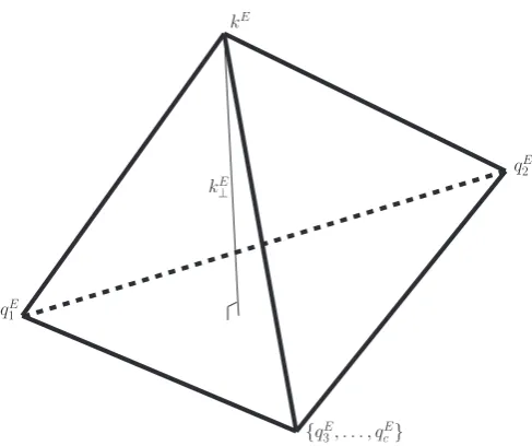
In this section we present a geometric interpretation of the final formula (3.31) for one-loop cut integrals in terms of the geometry of the polytopes determined by the external momenta together with the loop momentum. Our polytope picture reproduces a similar geometric picture in the works of Cutkosky in the case of the three-point function [1]. Let
JHEP06(2017)114
kEqE
2
{qE
3, . . . , qEc}
qE
1
[image:14.595.172.416.82.286.2]kE ⊥
Figure 1. The simplex KC whose base is the simplexQC, with the transverse component kE⊥ of
the loop momentum.
vectors emanating from the common pointqE
∗,∗ ∈C.4 Similarly,KC denotes thec-simplex
spanned by the edges{kE−qE
∗ , qiE−q∗E :i∈C\{∗}}(see figure1). Notice that the vertices
of these simplices correspond directly to the dual momentum variables. For definiteness, we assume without loss of generality that C = [c] andqE
∗ =q1E.
By construction, the polytope QC lives in the linear subspaceEC, and it is a face of the
simplex KC. The altitude of the polytope KC above the face QC is given by |k⊥|=|kE⊥|.
Our goal is to describe the geometrical properties of these two polytopes. We define the following matrices whose columns are formed by our momentum vectors,
QC = qE2 −q1E q3E −q1E · · · qcE−qE1
, (3.39)
KC = kE−qE1 qE2 −qE1 · · · qcE−q1E
, K∅ = kE
. (3.40)
Since it is preferable to work with Lorentz invariant expressions, we construct Gram de-terminants, and we can then write the volumes of the simplices in terms of their square roots. In particular, the Gram determinants that we are going to consider are
GramC = detQTCQC, Gram∅ = 1, (3.41)
HC = detKCTKC. (3.42)
It is easy to check that GramC andHCagree with the definitions of the Gram determinants
in eq. (3.24) and eq. (3.25). The volumes of the simplices can then be written as
volQC =
1
(c−1)!|GramC|
1/2 , (3.43)
volKC =
1
c!|HC| 1/2
. (3.44)
JHEP06(2017)114
We now use the fact that the volume of an N-simplex can be computed in two equivalent ways: first, by taking the determinant of the matrix whose columns are the edge vectors emanating from a common vertex, divided byN!, or second, by multiplying the volume of one of its (N −1)-dimensional faces by the altitude above that face, divided by N. We conclude that the altitude of the polytopeKC above the face QC is given by
|k⊥|=
HC
GramC
1/2
. (3.45)
So far, all the considerations are generic and apply independently of any propagators being cut. In the special case where the propagators from the setC are cut, we know that
|YC| = |[HC]C|, and we see that the height of KC is fixed by the on-shell conditions in
terms of the modified Cayley and Gram determinants,
[|k⊥|]C =
YC
GramC
1/2
. (3.46)
In other words, we see that the radius of the vanishing sphereS⊥=SC is fixed by eq. (3.46).
In order to understand the geometric meaning of eq. (3.46) and the nomenclature for the vanishing spheresSC and cycles ΓC, it is useful to understand the connection between
cut integrals and the Landau conditions [4], a set of necessary conditions on the external kinematics for a pinch singularity to occur. If we work in Euclidean kinematics, then the Landau conditions for a one-loop integral take the form
αi
(kE −qE
i )2+m2i
= 0, ∀i . (3.47)
and
n X
i=1
αi(kE−qEi ) = 0. (3.48)
The equations of the first Landau condition factorize: for each i, either αi = 0 or else
the propagator is on shell. Stated differently, if C is the set of cut propagators, the first Landau condition can be satisfied by settingαi= 0 for all i /∈C.5 After imposing the first
Landau condition, the second Landau condition can be restated as
X
i∈C
αi(kE−qEi ) = 0. (3.49)
In order to characterize the solution space of eq. (3.49), we can contract the equation with each momentum propagator (kE−qE
j ) for j∈C, giving the matrix equation
(kE−qE
1)·(kE −qE1) . . . (kE−qE1)·(kE−qEc )
..
. . .. ...
(kE−qE
c )·(kE −qE1) . . . (kE−qEc )·(kE−qEc )
α1 .. .
αc
= 0. (3.50)
JHEP06(2017)114
This linear system has a nontrivial solution only if its determinant vanishes. This deter-minant is the same as the Gram deterdeter-minant HC defined in eq. (3.24), except that the
momenta are Euclidean. We have seen that upon putting the propagators on-shell, HC
be-comes equal to the modified Cayley determinantYC. Equation (3.50) thus has a nontrivial
solution if and only ifYC = 0. These solutions to the Landau conditions, corresponding to
kinematic configurations where the modified Cayley determinant YC vanishes, are called
singularities of the first type.6
There is a nice geometric interpretation of the Landau conditions at one loop. The on-shell conditions force the volume of the polytope KC to be proportional to the (absolute
value of the) modified Cayley determinant YC. Hence, we see that the volume of KC
vanishes at points where both Landau conditions are satisfied. Moreover, we know from eq. (3.46) that the radius of the sphereSC is proportional to the square root ofYC, and so
we see that the radius of SC vanishes at the position of the pinch singularity. This is the
reason for the namesvanishing sphere and cycle for SC and ΓC =δCSC.
4 Explicit results for some cut integrals
In order to make the definitions of the previous section more concrete, we now present some explicit results for cut integrals. We give a concrete parametrization for the loop momentum with which the remaining integration in eq. (3.31) can be carried out. We identify conditions under which cuts can vanish identically and discuss their geometric interpretation. We then present some explicit results for maximal and next-to-maximal cuts.
4.1 Evaluation of the residues
We first introduce a parametrization of the loop momentum k such that the residues factorize and can be computed sequentially. To align the indices of the npropagators with those of the components of the momenta, we relabel the propagators from 0 to n−1 and using the Sn-symmetry of one-loop integrals, we assume without loss of generality that
the set of cut propagators isC ={n−1,0,1, . . . , c−2}, with all indices understood mod
n. In this section, C will always denote this set. We use momentum conservation to set
qE
n−1 =0D.
Throughout this section, we work with the Euclidean momenta introduced in eq. (3.32) and in a frame where
qjE = qEj0, . . . , qjjE,0D−j−1
, qjjE >0. (4.1)
We can parametrize the vector kE as
kE =r
cosθ0,cosθ1sinθ0, . . . ,cosθn−2
n−3
Y
j=0
sinθj,1D−n+1
n−2
Y
j=0 sinθj
, (4.2)
JHEP06(2017)114
where 1D−n+1 is a unit vector in (D−n+ 1) dimensions, r ≥ 0, and 0 ≤ θj < π. The
integration in the remaining (D−n+ 1) dimensions is trivial, and we obtain the following integration measure,
Z
dDk=i
Z
dDkE = iπ
D−n+1 2
Γ D−2n+1
Z
dr2 r2D−22 n−2
Y
j=0
Z π
0
dθjsinD−2−jθj. (4.3)
Next, for each angle θj, we change variables to tj = (cosθj+ 1)/2. The propagators
can be written as
(kE−qEj )2+m2j =−Aj(r, t0, t1, . . . tj−1) +tjBj(r, t0, t1, . . . tj−1). (4.4)
We then obtain the following expressions for Aj and Bj,
Aj = 2r
j−1
X
α=0
qEjα(2tα−1)
α−1
Y
γ=0 2
q
tγ(1−tγ)
−2jqjjE
j−1
Y
γ=0
q
tγ(1−tγ)
−m2j−(qjE)2−r2,
Bj =−2j+2rqjjE j−1
Y
β=0
q
tβ(1−tβ). (4.5)
Equations (4.4) and (4.5) make manifest the main property of our parametrization that allows us to evaluate all the residues sequentially. We see from eq. (4.4) that the propagators have only simple poles in the variables tj. Indeed, from eq. (4.5) we see that Aj and Bj
only depend on the tα with α < j, and so the position of the poles of the cut propagators
can easily be determined in terms of the variables tj. It is then easy to see that in this
parametrization the residues factorize, and so we can evaluate the residues sequentially at the simple poles in the tj. It will be useful to introduce the following notation for the
positions of the poles, corresponding to the values of the tj where eq. (4.4) vanishes,
Tj(r, t0, . . . , tj−1) =
Aj(r, t0, . . . , tj−1)
Bj(r, t0, . . . , tj−1)
. (4.6)
In terms of the functionsTj, the propagators in eq. (4.4) can be written as
(kE−qjE)2+m2j =Bj(r, t0, . . . , tj−1) [tj−Tj(r, t0, . . . , tj−1)] . (4.7)
Equation (4.7) shows that in our parametrization each propagator (kE −qE
j )2 +m2j is
naturally associated with a variable tj in which this propagator has a simple pole. The
only exception is the propagator (n−1), which is associated to the radial coordinater,
(kE)2+m2n−1 =r2+m2n−1. (4.8)
Before turning to the evaluation of the residues, it is instructive to see how the uncut integral looks in this parametrization. Since the integration contour is real and
sinθj = 2 q
JHEP06(2017)114
all the tj must vary in the range [0,1], and the uncut integral can be written as
In=(−1)n
2
Pn−2
j=0(D−2−j)eγE
πn−21Γ D−n+1
2
Z ∞
0
dr2 r
2D−22
r2+m2
n−1
n−2
Y
j=0
Z 1
0
dtj
[tj(1−tj)] D−3−j
2
Bj(tj−Tj)
, (4.10)
where we have dropped the dependence of the functions Bj and Tj on their arguments.
Let us now consider the cut integralsCCIn. We have already seen thatBj andTj only
depend on the radial coordinater and the tα withα < j. We can then easily evaluate the
residues by starting from the integrand of the uncut integral, eq. (4.10), and taking the residues at the poles of the cut propagators. In our parametrization, the position of the poles are defined iteratively by
r2 =−m2n−1 and tj =tj,p≡Tj q
−m2
n−1, t0,p, . . . , tj−1,p
. (4.11)
The cut integral CCIn is computed by sequentially taking the residues at each pole,
CCIn=
(2πi)bc/2ceγE
πn−21Γ D−n+1
2
2 Pc−2
j=0(D−2−j) × (4.12)
Resr2=−m2 n−1
Rest0=t0,p
. . .Restm−2=tm−2,p
r2D2−2
r2+m2
n−1
c−2
Y
j=0
[tj(1−tj)] D−3−j
2
Bj(tj−Tj)
fn c ,
wherefn
c collects the remaining (n−c) integrations,
fcn(r, t0, . . . , tc−2)≡2 Pn−2
j=c−1(D−2−j) n−2
Y
j=c−1
Z 1
0
dtj
[tj(1−tj)] D−3−j
2
Bj(tj−Tj)
, (4.13)
corresponding to the unconstrained variables tj with c−1 ≤ j ≤n−2 that vary in the
range [0,1], just as in the case of the uncut integral in eq. (4.10). We have suppressed the factor of (−1)n that appears in eq. (4.10) because we do not keep track of the overall sign of cut integrals, as discussed below eq. (3.30). We will continue to suppress other powers of −1 in the equations that follow.
The residues in eq. (4.12) involve only simple poles, and so they can all be easily evaluated sequentially by eliminating the relevant denominators and substituting the values of tj at the poles in the remaining expression, see eq. (4.11). We find that
CCIn= (2πi)bc/2c
2
Pc−2
j=0(D−2−j)eγE
πn−21Γ D−n+1
2
−m
2
n−1
D−22
[fcn]C c−2
Y
j=0
[tj,p(1−tj,p)] D−3−j
2
[Bj]C
. (4.14)
The function fn
c has been normalized such that in the case where all propagators are cut,
c = n, we have [fn
n]C = 1. Our goal is to identify [fcn]C with the integration over the
vanishing sphereSC in eq. (3.31),
[fcn]C = 2 Pn−2
j=c−1(D−2−j) n−2
Y
j=c−1
Z 1
0
dtj
[tj(1−tj)] D−3−j
2
[Bj]C(tj−[Tj]C)
= Γ
D−n+1 2
2πD−2n+1 Z
S⊥
dΩED−c+1
Y
j /∈C "
1 (kE−qE
j )2+m2j #
C
.
JHEP06(2017)114
kE
qE j
{qE
0, . . . , qEj−1}
0
φj
θj
r rsinφ
j
qj
{q0, . . . , qj−1}
0
[image:19.595.86.509.122.327.2]qjj
Figure 2. The simplexK[kE,0,1,2,...,j] and its base simplex Q[0,1,2,...,j], whose respective altitudes
arersinφj andqjjE.
In order to show that this is true, we need to show that the factors multiplying [fn c]C in
eq. (4.14) combine to give the modified Cayley and Gram determinants in eq. (3.31).
We consider the polytope picture of cut integrals introduced in section 3.4, adapted to our choice of frame. We use the notation of section 3.4, set qE
∗ =qnE−1 = 0, and keep C=
{n−1,0, . . . , c−2}as above. Our goal is to express some of the components of the momenta in the frame defined in eqs. (4.1) and (4.2) in terms of invariants. Since the parametrization in eqs. (4.1) and (4.2) relies on a specific ordering of the momenta qE
i , we denote by
Q[0,1,2,...,j] and K[kE,0,1,2,...,j] the simplices with edges {q0E, . . . , qjE} and {kE, q0E, . . . , qjE}
respectively, with the edges given in this order. These simplices are represented in figure2.
We observe that with the parametrization given in eq. (4.1) and eq. (4.2), each angle
θj can be interpreted as the dihedral angle between the facesK[kE,0,1,2,...,j−1]andQ[0,1,2,...,j]
in the simplexK[kE,0,1,2,...,j]. If we further letφj be the angle between the edgekE and the
faceQ[0,1,2,...,j], then
sinφj = j Y
k=0
sinθk. (4.16)
Now we examine the equivalent formulas for computing volumes. Consider the simplex
K[kE,0,1,2,...,j] and its face Q[0,1,2,...,j]. The altitude of the simplex above this face is the
distance from the endpoint ofkE toQ
[0,1,2,...,j], which isrsinφj. Similarly, we consider the
simplexQ[0,1,2,...,j]and its face Q[0,1,2,...,j−1]. The altitude of the simplex above this face is the distance from the endpoint ofqE
JHEP06(2017)114
j-th component qE
jj of the vector qjE. We obtain the following two relations,
rsinφj =
Yj1+2/2
Gram1j/+22
, qjjE = Gram 1/2
j+2
Gram1j+1/2
, (4.17)
where we use the shorthand Yj+2 ≡ Y{n−1,0,...,j}, and similarly for Gramj+2. Note that
rsinφj is just the altitude |k⊥|defined in section3.4.
In order to convert the expressions in eq. (4.14) to determinants, we observe that
ta,p(1−ta,p) = sin2θj/4 = sin2φj/(4 sin2φj−1), and that [Bj]C = −4rsinφj−1qjjE. As a
consequence of the relations above, we can write
r = Y11/2,
tj,p(1−tj,p) =
Yj+2Gramj+1 4Gramj+2Yj+1
,
[Bj]C =−
4Gram1j+2/2Yj1+1/2
Gramj+1
.
(4.18)
It is now straightforward to derive the following result.
CCIn = (2πi)bc/2c
21−ceγE
πn−21Γ D−n+1
2
1
√ µcY
C
µ YC
GramC D−2c
[fcn]C. (4.19)
Hence, comparing eq. (4.19) to eq. (3.31), we conclude that eq. (4.15) is proven (we recall that eq. (4.15) only holds in Euclidean kinematics).
4.2 Vanishing cuts
We will now state several conditions sufficient for the vanishing of one-loop cut integrals in dimensional regularization in generic kinematics, by which we mean that nonzero invariants are distinct.7 We define qij = qi −qj, and we introduce the following shorthand for
set-valued indices: if i, . . . , j are integers and C is a set of integers, then Ci...jIn denotes
C{i...j}In, andCCiIndenotesCC∪{i}In. Similar notation is used for the modified Cayley and
Gram determinants.
We have identified three classes of vanishing cut integrals. In these cases, at most three propagators are cut:
1) Single-cut integrals vanish if the cut propagator is massless:
CiIn= 0, ifm2i = 0. (4.20)
2) A double-cut integral vanishes if the momentum flowing through the cut is lightlike:
JHEP06(2017)114
3) A triple-cut integral vanishes if the cut isolates a three-point vertex where three lightlike lines meet:
CijkIn= 0, ifq2ij =m2i =m2j = 0. (4.22)
Let us discuss in turn the proofs of these claims, and let us start by showing that the single cut of a propagator of massm2
i vanishes in the limit m2i →0. We haveYi =m2i and
Grami = 1, and, using eqs. (3.31) and (4.15), the resulting cut integral is
CiIn=
eγE
πn−21Γ D−n+1
2
−m
2
i D−22
[f1n]i. (4.23)
This integral will vanish in dimensional regularization, unless [fn
1]ibehaves like (m2i)(2−D)/2
in the limit m2
i → 0. If this were the case, then [f1n]i would either be divergent or vanish
in the limit. We thus compute [fn
1]i form2i = 0 and check that it is finite (neither zero nor
divergent). From eq. (4.13) we get
[f1n]i = 2 Pn−2
j=0(D−2−j) n−2
Y
j=0
Z 1
0
dtj
[tj(1−tj)] D−3−j
2
[Bj]itj−[Aj]i
. (4.24)
For m2
i = 0, [·]i means the quantities inside the bracket should be evaluated at r = 0.
From eq. (4.5), we get
[Aj]i =Aj(r = 0) =−m2j −(qjE)2 and [Bj]i=Bj(r= 0) = 0. (4.25)
Hence, the integration in eq. (4.15) can be done in closed form, and we obtain
[f1n]i=π n−1
2 Γ
D−n+1 2
Γ D2
n−2
Y
j=0
m2j+ (qjE)2−1 , (4.26)
which shows that [fn
1]iis well behaved asm2i →0. This completes our proof of the vanishing
of the massless single cut.
Next, let us consider the conditions for a double cut to vanish. Consider the cut of two propagators of masses m2
i and m2j, the difference of whose momenta is qij. We have
Gramij = (qijE)2 and Yij =λ(m2i, m2j,(qEij)2)/4, where λdenotes the K¨all´en function,
λ(a, b, c) =a2+b2+c2−2(ab+ac+bc). (4.27)
The resulting cut integral is
CijIn =
i π3−2neγE
Γ D−2n+1 "
λ(m2
i, m2j,(qEij)2)
4
#D−23
(qEij)22−2D
[f2n]ij. (4.28)
By an argument similar to the previous case, we can see that this expression vanishes in dimensional regularization as (qE
ij)2 →0. Alternatively, one can see that this conclusion is
correct from eq. (4.12): if (qE
ij)2 = 0, then the corresponding propagator
(kE−qE
JHEP06(2017)114
k i
[image:22.595.233.362.83.201.2]j qij
Figure 3. Diagram representative of a triple cut.
is actually independent of t0 becauseB0(r) is zero for (qijE)2 = 0. In other words, there is no residue associated with t0, and so the cut integral vanishes.
Finally, let us turn to the vanishing of the triple cut. Consider the case where three propagators are cut, as depicted in figure 3, in a way that isolates a three-point vertex connecting three massless lines (in figure3, the vertex connecting the lines with labels i,j
and qE
ij). At one loop, the three massless lines must include two adjacent massless
propa-gators, labeled byiand j, and the external massless line incident to their common vertex carries the momentumqE
ij, such that (qEij)2 = 0. The choice of the third cut propagator is
unimportant, and it is labeled by k. The corresponding modified Cayley matrix takes the form
Yijk = det
0 0 m2k−(qikE)2
2
0 0 m
2 k−(qEjk)2
2
m2 k−(qikE)2
2
m2 k−(qjkE)2
2 m
2
k
= 0. (4.30)
The vanishing of the determinant in eq. (4.30) is due to a collinear singularity at the vertex where propagatorsiand j meet [42]. To conclude that the cut integral vanishes, we follow the same path as for one-propagator cuts and show that [fn
3]ijk is regular in this limit
(i.e., it neither vanishes nor diverges). To make the connection with the discussion in the previous section, we should relabel indices so that in figure 3 the propagators i, j and
k become respectively the propagators with index 0, 1 and n−1. Then, the collinearity condition corresponds to sinθ1 = 0, which through eq. (4.18) implies8 thatt1,p(1−t1,p) = 0.
We then have
[B2]ijk=−24rqE22
q
t0,p(1−t0,p) q
t1,p(1−t1,p) = 0, (4.31)
which in turn implies that [Bα]ijk = 0 for all α ≥2. The integration of the tα in [f3n]ijk
can thus be done in closed form, and we find
[f3n]ijk=π n−3
2 Γ
D−n+1 2
Γ D−22
n−2
Y
j=2
(−[Aα]ijk)−1 . (4.32)
JHEP06(2017)114
The last expression is finite, so the limitYijk→0 of [f3n]ijk is well defined. This completes
the proof of the vanishing of three-propagator cuts that isolate a massless three-point vertex.
The conditions listed above for one-propagator and three-propagator cuts illustrate that the vanishing of the vanishing sphere (cf. eq. (3.46)) leads to a vanishing cut. In this section, we have simply checked that this conclusion still holds in dimensional regularization when some scales are zero. On the other hand, the two-propagator cut vanishes when the corresponding Gram determinant does: this condition will be analyzed in section 5 in the context of second-type singularities.
We would like to emphasize that cuts such as the quadruple cut of a massless box do not fall into any of the above categories, and in fact this particular cut is nonzero. All of its three-propagator cuts vanish, for the reason given above. On the other hand, for the quadruple cut we have Y[4] =s2t2/16 and Gram[4] =−st(s+t)/4, and thus we find
C[4]Je40−mass = 2eγE
Γ(1−) Γ(1−2)
(s+t)
(s t)1+ . (4.33)
More generally, we have checked explicitly thatYCand GramC do not vanish for 4≤ |C| ≤8
in generic kinematic configurations, even in the case where all propagators and external legs are massless. Based on this observation, we conjecture that cuts of four or more propagators never vanish in generic kinematic configurations.
4.3 Explicit results for maximal cuts
In this section we show that the general formula (3.31) takes a particularly simple form when all propagators are cut, the so-calledmaximal cut. In this case, the remaining angular integration in eq. (3.31) is trivial, because the integrand does not contain any additional propagators. We look specifically at the class of one-loop integrals in even dimensions nearly matching the number of propagators, as specified in eq. (2.4). In section 8 we will see that these results suffice to compute the maximal cuts of arbitrary one-loop integrals.
We label the propagators from 1 to n and distinguish the cases of neven and n odd. Forn even, we find
C[n]Jen= 21−2− n 2i
n 2 e
γEΓ(1−)
Γ(1−2) 1
p
Y[n]
Y
[n] Gram[n]
−
, neven. (4.34)
Forn odd, we find,
C[n]Jen= 2 1−n
2 i n−1
2 e γE
Γ(1−) 1
p
Gram[n]
Y
[n] Gram[n]
−
, nodd. (4.35)
JHEP06(2017)114
to lower point integrals. Conversely, we have argued that cut integrals with four or more cut propagators never vanish in generic kinematics, and so we expect that integrals with four or more propagators cannot be reduced to lower point integrals.
4.4 Explicit results for next-to-maximal cuts
Cut integrals with all but one of the propagators cut, the so-called next-to-maximal cuts, also admit a particularly simple closed expression. We first discuss a general integral In,
and then restrict our analysis to the basis integrals Jen. The discussion in this section is
valid if the maximal cut does not vanish.
We label the propagators from 1 to nand assume without loss of generality that the set of cut propagators is C = [n−1]. In the case of a next-to-maximal cut the remaining angular integral can be carried out in terms of Gauss’s hypergeometric function,
2F1(a, b;c;z) =
Γ(c) Γ(b)Γ(c−b)
Z 1
0
dt tb−1(1−t)c−b−1(1−zt)−a. (4.36)
From eq. (4.15), we find
[fnn−1]C =−
2D−nΓ2 D−2n+1
tp[B]CΓ(D−n+ 1)
2F1
1,D−n+ 1
2 ;D−n+ 1; 1
tp
. (4.37)
Using the relation [43]
2F1(a, b; 2b;z) = (1−z)−
a 2 2F1
a
2, b−
a
2;b+ 1 2;−
z2 4(1−z)
, (4.38)
and the fact that eq. (4.18) implies
tp(1−tp) =
Y[n]Gram[n−1] 4Gram[n]Y[n−1]
, (4.39)
we observe that the left-hand side of eq. (4.37) can be written entirely in terms of Gram and modified Cayley determinants:
[fnn−1]C=
2D−n−1Γ2 D−2n+1 Γ(D−n+ 1)
s
−GramY [n−1]
[n] 2F1
1 2,
D−n
2 ;
D−n+ 2
2 ;
Gram[n]Y[n−1] Gram[n−1]Y[n]
.
(4.40) Inserting this result into eq. (3.31), we easily find that the next-to-maximal cut of a diagram withn propagators is
C[n−1]In= (2πi)b n−1
2 c2
D−2n+1eγEΓ D−n+1 2
πn−21Γ(D−n+ 1)
1
p
−Y[n]
Y
[n−1] Gram[n−1]
D−2n
2F1
1 2,
D−n
2 ;
D−n+ 2
2 ;
Gram[n]Y[n−1] Gram[n−1]Y[n]
.
(4.41)
JHEP06(2017)114
in dimensional regularization can be expressed in terms of polylogarithmic functions. We next present an alternative way to write the next-to-maximal cut of the basis integrals Jen
where all the indices of the 2F1 function are integers as →0, and so all the coefficients in the Laurent expansion are polylogarithmic. The price to pay is that the arguments of the polylogarithms involve square roots. Equation (4.39) implies that
tp =
1 2
1±p
1−η, (4.42)
where we define
η≡ Y[n]Gram[n−1]
Gram[n]Y[n−1]
. (4.43)
For concreteness, we assume in the following that 0 < η < 1 and choose the solution of eq. (4.39) with a plus sign. The results of other choices can be obtained by analytic continuation, and they would be equivalent modulo iπ.
Let us separate the cases where n is even or odd. If nis odd, eq. (4.37) immediately gives
C[n−1]Jen=−2 3−n
2 −2i n−1
2 e
γEΓ(1−)
Γ(2−2)
Y
[n−1] Gram[n−1]
−
1
p
Gram[n]
× 1
1 +√1−η2F1
1,1−; 2−2; 2 1 +√1−η
, nodd.
(4.44)
We see that the hypergeometric function has integer indices. Its Laurent expansion in
can therefore be expressed in terms of polylogarithms to all orders [44]. The first order is:
C[n−1]Jen=
21−2ni n−1
2 p
Gram[n] log
p
Y[n]Gram[n−1]−Gram[n]Y[n−1]−
p
−Gram[n]Y[n−1]
p
Y[n]Gram[n−1]−Gram[n]Y[n−1]+
p
−Gram[n]Y[n−1]
!
+O()
(4.45) Ifnis even, a convenient representation of the hypergeometric function is obtained by applying the following transformation [43] to eq. (4.37),
2F1(a, b; 2b;z) =
1 +√1−z
2
−2a
2F1 a, a−b+ 1 2;b+
1 2;
1−√1−z
1 +√1−z
2!
. (4.46)
The next-to-maximal cut of Jen withn even is then given by
C[n−1]Jen =−21− n 2i
n−2 2 e
γE
Γ(1−)
Y
[n−1] Gram[n−1]
− p
Gram[n−1]
p
Gram[n]Y[n−1]
1
√
1−η+√−η
× 2F1
1,1 +; 1−;
√
1−η−√−η √
1−η+√−η
, neven.
(4.47)
We again see that we can express the next-to-maximal cut in terms of hypergeometric functions with integer indices only. The first orders are
C[n−1]Jen=−
2−n2 i n 2 p
Y[n] 1 + 2log 1 +
s
Y[n]G[n−1]−G[n]Y[n−1]
Y[n]G[n−1]
!
+ (4.48)
log
G
[n−1] 4Y[n−1]
+O 2
JHEP06(2017)114
Let us conclude this section by highlighting a relation between the maximal and next-to-maximal cuts of a one-loop integral with an even number of propagators. Expanding the explicit results for these cuts in eqs. (4.34) and (4.47) to leading order in the dimensional regulator, we find
C[n−1]Jen=−
1
2C[n]Jen+O() , neven. (4.49) In principle, the sign in this relation is not determined, as our cuts are defined up to an overall sign as discussed below eq. (3.31). Imposing the minus sign in eq. (4.49) fixes the relative sign between maximal and next-to-maximal cuts of integrals with even number of propagators. In the next section, we will see that this relation is a special case of a larger class of relations between cut integrals. Finally, we stress that eq. (4.49) only holds if both sides of the equality are well defined at = 0.
5 Compactification and singularities of the second type
In addition to pinch singularities, Feynman integrals may also exhibit singularities when the integration contour is pinched at infinity [2,29,30]. These so-calledsingularities of the
second typeare classified by the vanishing of the Gram determinant GramC (see appendixB
for a derivation) rather than the modified Cayley determinant,9 and they are not directly related to the cut integrals as defined above.
However, the notion of cut integrals can indeed be extended to singularities of the second type. In this section, we will make this statement precise by performing a compact-ification and considering residues at infinity. In the compactified picture, singularities of the first and second types can be treated on the same footing. Furthermore, for one-loop integrals, the so-called Decomposition Theorem [31, 32, 45] implies that cut integrals for singularities of the two types are not independent, leading to various linear relations among cut integrals.
5.1 Compactification of one-loop integrals
In previous sections, we have seen that to every singularity of the first type defined by
YC = 0 we can associate the cut integralCCInD. In order to extend these concepts to the
singularities of the second type, the usual momentum representation of loop integrals is not the most convenient, because the pinch happens at infinite loop momentum. We therefore use a representation of one-loop integrals as integrals over a compact quadric in the complex projective space CPD+1 [31, 46,47], which we review in this subsection. Throughout this section we work in Euclidean kinematics, and we strictly follow the conventions of ref. [46]. We write pointsZ inCPD+1 in terms of homogeneous coordinates as
Z =
zµ
Z− Z+
, (5.1)
JHEP06(2017)114
and we identifyZ and α Z, withα∈C,α6= 0. We equip CPD+1 with the bilinear form
(Z1Z2) =zµ1z2µ−
1 2Z
+ 1 Z
− 2 −
1 2Z
− 1 Z
+
2 , (5.2)
where zµ1z2µ denotes the usual Euclidean scalar product. If we work in the coordinate
patch Z+ = 1, then to each propagator D
i = (kE −qEi )2 +m2i we associate the point
Xi∈CPD+1 defined by
Xi =
(qE i )µ
(qE
i )2+m2i
1
, 1≤i≤n . (5.3)
Note that (XiXi) =−m2i <0 for positive values of the masses. The one-loop integral InD
can then be written as an integral over the D-form$D n,
InD =
Z
Σ
$Dn , with$Dn = (−1)
neγE
πD/2
dD+2Y δ((Y Y)) Vol(GL(1))
[−2(X∞Y)]n−D
[−2(X1Y)]. . .[−2(XnY)]
, (5.4)
where Σ is the real quadric defined by (Y Y) = 0 (take e.g.Y = [(kE)µ,(kE)2,1]T), and we
have introduced the ‘point at infinity’
X∞=
0µ 1 0
. (5.5)
The singular surfaces where the propagators go on shell are mapped to the hyperplanesPi
in CPD+1 defined by (XiY) = 0, i∈ [n]. There is an additional singular hyperplane P∞
defined by (X∞Y) = 0. In the compactified picture, the solutions to the Landau conditions
are classified by the vanishing of the Gram determinants det(XiXj)i,j∈C, where nowC is a
subset of{1, . . . , n,∞}. These determinants are related to the original Gram and modified Cayley determinants defined in eq. (3.25) and eq. (3.29) by
det(XiXj)i,j∈C = (
(−1)cYC, if∞∈/ C ,
(−1)c−1
4 GramC\{∞}, if∞ ∈C .
(5.6)
After compactification, there is no distinction between the Landau singularities of the first and second type: they are treated on the same footing. The compactification of one-loop integrals thus provides the ideal framework to extend the notion of cut integrals to Landau singularities of the second type. However, there are two issues which we need to address in order to precisely define the cut integrals associated with these singularities:
1) We need to know the vanishing spheres and cycles in the compactified picture, because they provide the integration contours for cut integrals.
2) In dimensional regularization, the integrand $D
n has a ‘branch point’ on P∞ rather
than a pole, as seen from the factor of (X∞Y)n−D. Hence, we cannot apply the
residue theorem (3.8) which was crucial in the derivation of eq. (3.38).
JHEP06(2017)114
5.2 Homology groups associated to one-loop integrals
Working in the compactified picture, we need to identify the vanishing spheres ˜SC and
van-ishing cycles ˜ΓC in order to understand one-loop cut integrals, according to the discussion
of section 3. We use a tilde to distinguish the vanishing spheres and cycles in the com-pactified picture from those in the momentum space picture, and we denote the complex quadric (Y Y) = 0 by Σ, in contrast to the real quadric Σ of the previous subsection.
The vanishing spheres and cycles are most conveniently characterized by studying the homology groups of Σ−P∞−P[n] where
PC ≡ [
j∈C
Pj and PC ≡ \
j∈C
Pj, C ⊆[n]∪ {∞}. (5.7)
Very loosely speaking, homology groups classify all the non-equivalent integration contours that we can define on a space. The homology groups relevant to one-loop integrals10 have been studied in refs. [31, 32, 45], where it was shown that they are one-dimensional and generated by all the cycles that wind around11 Pj, withj6=∞. The rest of this subsection
consists of a short review of this result.
We identify CD+1 with the coordinate patchZ+ = 1 and define Σ0 ≡Σ∩CD+1. We will be interested in the surfaces Σ0∩PC. Since Σ
0
is a quadric and PC is an intersection
of hyperplanes, each Σ0 ∩PC is a projective (D−c)-dimensional quadric, with c = |C|,
which is necessarily compact. Consider now the homology groups HD−c(Σ 0
∩PC): they
are one-dimensional and g
![Figure 2. The simplex K[kE,0,1,2,...,j] and its base simplex Q[0,1,2,...,j], whose respective altitudesare r sin φj and qEjj.](https://thumb-us.123doks.com/thumbv2/123dok_us/974804.610862/19.595.86.509.122.327/figure-simplex-base-simplex-respective-altitudesare-sin-qejj.webp)

