Computational Methods for Bayesian Inference in Complex Systems

(1)

Complex Systems

Thesis by

Thomas Anthony Catanach

In Partial Fulfillment of the Requirements for the degree of

Doctor of Philosophy

CALIFORNIA INSTITUTE OF TECHNOLOGY Pasadena, California

2017

(2)

Thomas Anthony Catanach ORCID: 0000-0002-4321-3159

(3)

ACKNOWLEDGEMENTS

I would first like to thank my advisor, Prof. Jim Beck. Jim has shaped how I think about the world by introducing me to the Bayesian perspective and has been an excellent role model. He has demonstrated how to effectively bridge pure and applied research and helped me develop the tools I need for my future career. Further, I have truly enjoyed talking with him about a whole range of topics from the geography of New Zealand to the Bayesian perspective on quantum physics.

I am also very thankful to the faculty of Caltech who have been instrumental in guiding me and my work. I would like to thank my thesis committee members, Prof. Andrew Stuart, Prof. Mark Simons, and Prof. Steven Low. Their input in my work and knowledge of their respective fields has been most helpful. The classes I took during graduate school really transformed how I think about my research, particularly those in CDS and probability. Therefore, I would like to thank Prof. Richard Murray, Prof. John Doyle, and Prof. Houman Owhadi.

The CMS department and the general Caltech community has been a great place to work. I would like to thank Maria, Sydney, Carmen, and Nikki for all your help. I would also like to thank Armeen, Noah, Utkan, Pinaky, Yong Sheng, Yoke Peng, Tony, Yorie, Niangjun, Ioannis, and Mickey. My friends here at Caltech have been great people to share this experience with. I have really benefitted from your company and your friendship.

I would also like to thank the Department of Energy Computational Science Graduate Fellowship program for providing me with both funding and guidance. I really enjoyed the two summers I spent working at Los Alamos National Laboratory and would like to thank Earl Lawrence, Russell Bent, and Scott Vander Wiel and all my other colleagues there.

(4)

both how to love and how to learn. I have also been blessed to have two wonderful sisters, Therese and Maria. I have really enjoyed all the trips and times we have had together. Therese has been my partner in crime and Maria has been there to get us out of trouble when we needed it. I am happy that we share so much.

(5)

ABSTRACT

Bayesian methods are critical for the complete understanding of complex systems. In this approach, we capture all of our uncertainty about a system’s properties using a probability distribution and update this understanding as new information becomes available. By taking the Bayesian perspective, we are able to effectively incorpo-rate our prior knowledge about a model and to rigorously assess the plausibility of candidate models based upon observed data from the system. We can then make probabilistic predictions that incorporate uncertainties, which allows for better de-cision making and design. However, while these Bayesian methods are critical, they are often computationally intensive, thus necessitating the development of new approaches and algorithms.

In this work, we discuss two approaches to Markov Chain Monte Carlo (MCMC). For many statistical inference and system identification problems, the development of MCMC made the Bayesian approach possible. However, as the size and complex-ity of inference problems has dramatically increased, improved MCMC methods are required. First, we present Second-Order Langevin MCMC (SOL-MC), a stochas-tic dynamical system-based MCMC algorithm that uses the damped second-order Langevin stochastic differential equation (SDE) to sample a desired posterior dis-tribution. Since this method is based on an underlying dynamical system, we can utilize existing work in the theory for dynamical systems to develop, implement, and optimize the sampler’s performance. Second, we present advances and theoret-ical results for Sequential Tempered MCMC (ST-MCMC) algorithms. Sequential Tempered MCMC is a family of parallelizable algorithms, based upon Transitional MCMC and Sequential Monte Carlo, that gradually transform a population of sam-ples from the prior to the posterior through a series of intermediate distributions. Since the method is population-based, it can easily be parallelized. In this work, we derive theoretical results to help tune parameters within the algorithm. We also introduce a new sampling algorithm for ST-MCMC called the Rank-One Modified Metropolis Algorithm (ROMMA). This algorithm improves sampling efficiency for inference problems where the prior distribution constrains the posterior. In particular, this is shown to be relevant for problems in geophysics.

(6)

(7)

PUBLISHED CONTENT AND CONTRIBUTIONS

[Bae+16] Ania-Ariadna Baetica, Thomas Anthony Catanach, Victoria Hsiao, Richard Murray, and James Beck. “A Bayesian approach to inferring chemical signal timing and amplitude in a temporal logic gate using the cell population distributional response”. In:bioRxiv(2016), p. 087379. TA Catanach developed this problem in the Bayesian framework and the computational methods used to solve it. The method presented in this paper is used in Chapter 5.

[CB17] Thomas A Catanach and James L Beck. “Bayesian System Identifi-cation using Auxiliary Stochastic Dynamical Systems”. In: Interna-tional Journal of Non-Linear Mechanics (2017). doi: 10 . 1016 / j . ijnonlinmec.2017.03.012. url:https://doi.org/10.1016/ j.ijnonlinmec.2017.03.012.

TA Catanach developed, implemented, and tested the SOL-MC method. These results are presented in Chapter 2.

[Gar+15] M. Garcia, T. Catanach, S.V. Wiel, R. Bent, and E. Lawrence. “Line Out-age Localization Using Phasor Measurement Data in Transient State”. In:Power Systems, IEEE Transactions onPP.99 (2015), pp. 1–9. issn: 0885-8950. doi:10.1109/TPWRS.2015.2461461.

(8)

LIST OF ILLUSTRATIONS

Number Page

1.1 Bayesian updating for the system description swith the prior distri-bution p(s)to the posterior distributionp(s | D)given dataD . . . . 2 1.2 Graphical Model of Bayesian Filtering/State Estimation . . . 6 1.3 Graphical Model of Bayesian Parameter Estimation . . . 6 1.4 Graphical Model of Bayesian Model Selection . . . 7 1.5 A layered Bayesian approach for fast and flexible estimation and control. 9 1.6 Illustration of the evolution of a Markov chain for Metropolis-Hastings

MCMC. . . 12 2.1 Illustration of the evolution of HMC for a 1D Gaussian posterior. The

level sets of the Hamiltonian are seen in gray. The red trajectories illustrate the evolution of the system along a level set according to Hamiltonian dynamics. The green steps illustrate momentum resampling, which changes the level set. . . 19 2.2 Illustration of the trade-off of choosing the damping. If there is very

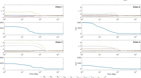
little damping, Hamiltonian dynamics dominate resulting in a highly correlated trajectory that can quickly explore the space. If there is high damping, the OU process dominates which results in less coherent evolution but also less exploration of the space. For optimal damping, the trajectories balances the drift and diffusion processes to explore the space without excessive correlation. . . 22 2.3 Position and potential energy trajectories of the four chains. . . 30 2.4 Sample trajectories projected onto theσ2andαplane where the color

indicates the evolution in time moving from blue to red. . . 32 2.5 Sample trajectories projected onto the σ2 and ru,3 plane where the

color indicates the evolution in time moving from blue to red. . . 33 2.6 Samples showing parameter distributions and correlation for the

glob-ally identifiable case using SOL-MC. . . 35 2.7 Plots of the minimum effective sample size for 1000 samples over

(11)

2.8 Samples showing parameter distributions for the unidentifiable case using SOL-MC. The colors represent the ten chains. . . 37 2.9 Samples showing parameter correlations for the unidentifiable case

using SOL-MC. The colors represent the ten chains. . . 38 2.10 Autocorrelation for the Hamiltonian and SOL-SDE dynamics defined

by a Gaussian posterior with imperfectly estimated covariance structure. 40 2.11 Mean and Covariance Estimate Error when using HMC, fixed

damp-ing SOL-MC, and fixed dampdamp-ing SOL-MC with momentum resam-pling (MR). The points indicate implementations with different pa-rameters and their error bars. The lines show the Pareto optimal performance front for each algorithm. . . 41 2.12 Mean and Covariance Estimate Error when using HMC, SOL-MC

with adaptive damping, and SOL-MC with momentum resampling (MR) and adaptive damping. The points indicate implementations with different parameters and their error bars. The lines show the Pareto optimal performance front for each algorithm. . . 42 2.13 Mean and Covariance Estimate Error when using RM-HMC,

Rie-mannian SOL-MC, and RieRie-mannian SOL-MC with momentum re-sampling (MR). The points indicate implementations with different parameters and their error bars. The lines show the Pareto optimal performance front for each algorithm. . . 43 3.1 Illustration of a set of distributions which gradually transform a

uni-modal prior into a biuni-modal posterior. These intermediate distribu-tions are defined by an annealing factor β ∈ [0,1] . . . 46 3.2 Illustration of finding∆βthat defines how much additional influence

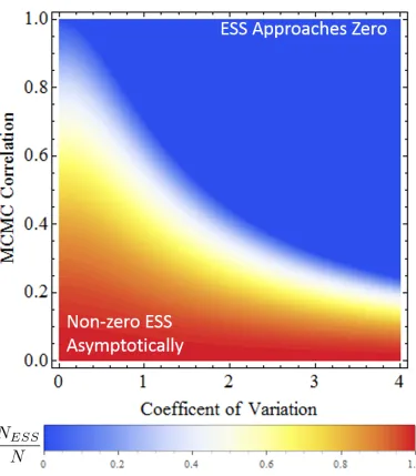
the data has in the next intermediate distribution level. Red dots indicate the sample and their size indicates their weight. If too large a ∆β step is made, only a few samples will have the majority of the weights, indicating that the samples poorly represent the distribution. If too small a∆βstep is made, the next distribution is too close to the current distribution making it an inefficient choice. . . 48 3.3 Asymptotically, with respect to the number of levels, the ratio of the

(12)

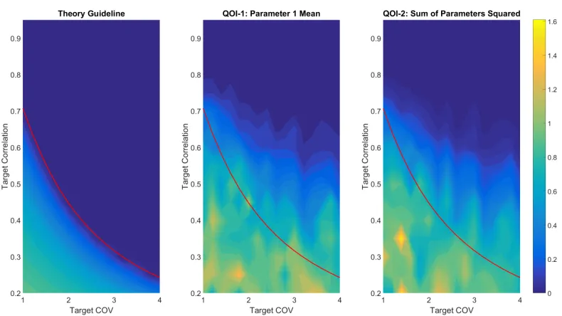
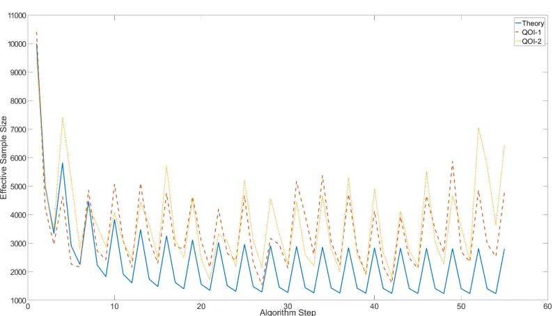
3.4 Comparison of the ratio of ESS to total number of samples for the theoretical results, equation (3.16), and the results for two actual quantities of interest computed by simulation. The red line is the theoretical learning cutoff. . . 56 3.5 Trajectory of the ESS during a run of ST-MCMC for two quantities

of interest, along with the theoretical trajectory. . . 57 3.6 Change factor in the ESS for each step in the ST-MCMC algorithm

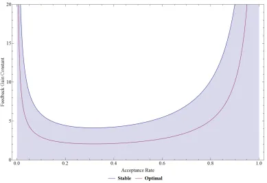
for the two quantities of interest along with the theoretical change factor. Green corresponds to the MCMC step, red the resampling step, and blue the importance weighting step. . . 58 3.7 Stability region of the linearized system for different target acceptance

rates. The optimal rate corresponds to critical damping. . . 66 3.8 Comparison of log scaling factor trajectories for different feedback

controller gains corresponding to underdamped (yellow), critically damped (red), and overdamped (blue). . . 67 3.9 Empirical relationship between proposal scaling factor and

accep-tance rate (left panel) and accepaccep-tance rate and correlation (right panel) for different acceptance rate values. . . 72 3.10 Histograms for the 49 parameters from the sample population of

Random Walk Metropolis, the Modified Metropolis Algorithm, and the Rank One Modified Metropolis Algorithm for the constrained Bayesian logistic regression problem. . . 78 3.11 Required number of forward model evaluations using Random Walk

Metropolis, the Modified Metropolis Algorithm, and the Rank One Modified Metropolis Algorithm to solve the constrained Bayesian logistic regression problem. . . 79 3.12 Sample Mean and Standard Deviation of the final sample population

using Random Walk Metropolis, the Modified Metropolis Algorithm, and the Rank One Modified Metropolis Algorithm for the static finite fault model parametersθk. . . 80

3.13 Histograms of the final sample population using Random Walk Metropo-lis, the Modified Metropolis Algorithm, and the Rank One Modified Metropolis Algorithm for the static finite fault model parametersθk. . 81

(13)

3.15 Required number of forward model evaluations using Random Walk Metropolis, the standard Rank One Modified Metropolis Algorithm, and the Adaptive Rank One Modified Metropolis Algorithm for an unconstrained Bayesian logistic regression problem. . . 83 4.1 A layered approach for fast power system estimation and control based

upon a Bayesian learning architecture. The shaded boxes describe inference methods developed in this work. . . 88 4.2 37-bus test system with nine generators on seven buses (Yellow). . . . 100 4.3 Comparison of the performance of fault handling methods for

differ-ent fault durations. RMSE is averaged over all states for a five second trajectory. . . 101 4.4 Performance comparison of integration methods. Each circle

corre-sponds to an estimator that uses different parameters for the numerical integrator. The computation time is measured relative to the length of the time period simulated. . . 102 4.5 Performance of the Extended Kalman Filter (EKF), Unscented Kalman

Filter (UKF), and Particle Filter (PF) for different specifications of modeled process noise and given an actual process noise level of 10−1. 104 4.6 Performance of the EKF (blue), UKF (red), and PF (orange) with

respect to the sampling and integration time step. . . 105 4.7 Estimator performance under different sampling rates and

measure-ment error intensities . . . 106 4.8 Performance impact of using additional PMUs for the local-global

state estimator, the figure shows the average error (red) over all pos-sible bus faults (grey). . . 107 4.9 Performance of the hybrid estimator for a large 148 bus system for

faults on buses 15, 31, 45, 87, and 110, lasting between 0.01 and 0.32 seconds. . . 108 4.10 a) Comparison of the estimator for tracking a stable (blue) and

unsta-ble (red) trajectory. b) Small-signal stability analysis for the system . 109 4.11 False detection rate for different levels of threshold and prior fault

probability. . . 110 4.12 Example fault detection for a cleared fault. . . 110 4.13 Example fault classification as more data is integrated. Colors

(14)

4.14 Illustration of dividing a power system into two partitions. The power flows on lines connecting the two regions are modeled as uncertain inputs. The voltage phasor on the input bus with the swing bus is also fixed. . . 112 4.15 Collection of Seven 37-bus subsystems arranged in a cycle. A fault

occurs in subsystem 4 and breakers on the lines 3-4 and 5-6 open to temporarily split the cycle into two connected components. . . 114 4.16 Comparison of the estimated (Red) and true dynamic states (Blue) of

the generator on Bus 31 of subsystem 1. The estimated one standard deviation uncertainty is shaded red. . . 116 4.17 Comparison of the estimated (Red) and true dynamic states (Blue)

for one of three generators on Bus 54 of subsystem 1. The estimated one standard deviation uncertainty is shaded red. . . 117 5.1 Graphic demonstrating the heterogeneous cell population response to

two chemical inputs. Colors indicate different cell florescent outputs. 119 5.2 We restrict the chemical inducer inputsa andbto be square waves.

They turn on at timestaON andtbON and turn off at timestaOFF and tbOFF. . . 122

5.3 The probabilistic model used to construct the likelihood of the ob-served data is based on two sources of uncertainty: model prediction uncertainty and random sampling errors. . . 125 5.4 Histograms of the posterior sample and kernel density plots showing

the correlation in the posterior for Case 1. . . 128 5.5 Histograms of the posterior sample and kernel density plots showing

the correlation in the posterior for Case 2. Note that the scale on the axes differ from Figure 5.4. . . 129 5.6 Histograms of the posterior sample and kernel density plots showing

the correlation in the posterior for Case 3. . . 130 5.7 Histograms of the posterior sample and kernel density plots showing

(15)

LIST OF TABLES

Number Page

2.1 Summary of the statistics for the four Markov Chains describing the effective sample size of each chain of length 2000 samples, total effective number of samples out of 8000 samples, mean estimate for each variable scaled relative to the true value, and the standard

deviation. . . 34

2.2 Summary of the statistics for the ten Markov Chains describing the effective sample size of each chain of length 2000 samples, total effective number of samples out of 20000 samples, mean estimate for each variable scaled relative to the true value and the scaled standard deviation. . . 39

5.1 The table describes the inputs, DNA states, and outputs to the event detector. Table adapted from [Hsi+16]. . . 121

5.2 The variables,θ, parameterize the event that chemical inducersaand bare added based upon the start time, end time, and magnitude. . . . 124

5.3 Posterior estimates for Case 1 . . . 128

(16)

C h a p t e r 1

INTRODUCTION TO BAYESIAN METHODS

Bayesian methods for identification and estimation are critical to the robust un-derstanding of a system because they allow us to quantify all of our uncertainty about the system using a probability distribution and to update this distribution with new information [BK98; BA02; Ves08; Bec10; Yue10b; Yue10a; WH12; APK15; GW15]. By taking the Bayesian approach, we are able to effectively capture our prior knowledge about a model and rigorously assess the plausibility of candidate model classes based on system data. Finally, we can then make robust probabilistic predictions that incorporate all uncertainties, allowing for better decision making and design. This robust approach is particularly relevant for complex system iden-tification, where the inverse problems are often ill-posed, many candidate models exist to describe the behavior of a system, and stochastic models are common.

1.1 Bayesian Inference

The Bayesian framework is a rigorous probabilistic method for representing uncer-tainty using probability distributions. This philosophy is rooted in probability as a logic [Bec10; Cox46; Cox61; Jay03]. Within this framework, probability distribu-tions are used to quantify uncertainty due to insufficient information, regardless of whether that information is believed to exist but is currently not available (epistemic uncertainty), or it is believed to not exist because of postulated inherent randomness (aleatory uncertainty). This notion of uncertainty makes the Bayesian framework the appropriate framework for posing system identification problems, where postu-lated system models have parameters whose values are uncertain rather than random. Therefore, we view system identification as updating a probability distribution that represents our beliefs about models of a system based on new information from system response data.

In general, the Bayesian inference problem uses Bayes’ theorem to update the understanding of a system using data, where understanding means assigning a probability function p()to different system descriptions. This updating process is visualized in Figure 1.1. The inference problem is formulated as follows: Given output measurementszi ∈ D, whereD is the set of data, and a system description,

(17)

Figure 1.1: Bayesian updating for the system descriptionswith the prior distribution

p(s)to the posterior distributionp(s | D)given dataD

p(D | s), describing the plausibility of the data given the description s, and (b) a prior distribution, p(s), representing the beliefs about the relative plausibility of

s, find the posterior distribution p(s | D) that represents the updated belief after integrating the observational data. For this, Bayes’ Theorem is used:

p(s | D)= p(D | s)p(s)

p(D) . (1.1)

The likelihood function,p(D | s), is the likelihood of observing the dataD given the model of the system. This model in the Bayesian framework maps s to a probability distribution on the outputs zi. The normalizing factor in equation (1.1),

p(D), is

p(D)=

∫

S

p(D | s)p(s)ds (1.2)

(18)

significant challenge to computational Bayesian methods since it is often difficult to find and explore all the peaks or the manifold of plausible solutions.

1.2 Bayesian Methods for Complex Systems

Inference Problems

Bayesian inference, as introduced in Section 1.1, for complex systems can broadly be divided into three fundamental problems: state estimation, parameter estimation, and model selection. These problems are interconnected and solving one cannot be done without assuming a solution to the others or solving them simultaneously. Together, these processes describe a hierarchy of Bayesian inference problems for dynamical systems, which we can use to design a Bayesian inference architecture.

This work considers both static and dynamic systems that can be described by a specific modelM or a discrete set of possible models also called model classes,Mi

fori = 1...N. These models may be informed by an understanding of the physics of the complex system or by some set of functions that are believed to capture the space of possible behaviors of the system.

In the model selection problem, the likelihoods of different modelsM_ifori= 1...N

can be computed based upon the data from a system, D. The probability of any modelMi, given observational dataD, is defined asp(Mi | D). Assuming the prior

probability of a model is known and defined as p(Mi) such that ÍN_i p(Mi) = 1,

then the posterior is

p(M_i | D)= p(D | Mi)p(Mi)

p(D) (1.3)

Using the law of total probability:

p(Mi | D)=

p(D | Mi)p(Mi) ÍN

j p Mj

p M_j (1.4)

(19)

Applying the Bayesian inference formulation to parameter estimation and sys-tem identification yields the description of Bayesian syssys-tem identification given in [Bec10]: Given observation data D, and assuming a system model class M∗ consisting of (a) a likelihood function p(D | θ,M∗), describing the plausibility of the data given a set of parameters, θ, and (b) a prior distribution, p(θ | M∗), representing the initial beliefs about the relative plausibility of the possible values of the model parameter vector θ, find the posterior distribution p(θ | D,M∗)that represents the updated beliefs as

p(θ | D,M∗)= p(D | θ,M

∗₎

p(θ | M∗)

p(D | M∗₎ (1.5)

The normalizing factor in equation (1.5),p(D | M∗), is the evidence for the model classM∗. The evidence can be computed as

p(D | M∗)=

∫

p(D | θ,M∗)p(θ | M∗)dθ (1.6)

This evidence can then be used in Equation 5.13 to solve the corresponding model class section problem if multiple model classes exist to describe the behavior.

The parameter estimation or system identification problem is the most typical formu-lation for Bayesian inference. It captures static systems and deterministic dynamical systems. However, for a stochastic dynamical system, where the observed behavior of the system is a function of the state of the system, x(t), and an unknown input modeled as a stochastic process, estimating this internal state is itself a Bayesian inference problem called state estimation or Bayesian filtering.

State estimation is the process of using measurements from a stochastic dynamical system to infer the dynamical states. Assuming the measurements are available at discrete times, it is appropriate to treat the system as a discrete time system:

xk =F(xk−1,wk, θ,M∗) zk =H(xk, νk, θ,M∗)

(1.7)

Here,F(x,w, θ,M)is the discrete stochastic dynamic state evolution function from model classM and parameterized byθ, whileH(x,w, θ,M)is the stochastic mea-surement function also from model classM and parameterized byθ. At timetk for

(20)

an unknown stochastic input, while νk is an unknown measurement disturbance or

error.

State estimation can be done using the Bayes Filter, where the posterior distribution

p(xk | z1:k)is updated from the prior state estimate distributionp(xk | z1:k−1)using

the measurements up to timetk represented asz1:k. Using Bayes’ Theorem and the

Markov property, the posterior is found recursively by applying two equations:

First prediction ofxk givenz1:k−1:

p(xk | z1:k−1)= ∫

p xk | x0_k₋₁p x_k0₋₁ | z1:k−1dx0k−1 (1.8)

Then the correction step integrates the new observations, so the prediction of xk

givenz1:k is

p(xk | z1:k) ∝ p(zk | xk)p(xk | z1:k−1) (1.9)

This inference problem can be visualized through the graphical model in Figure 1.2. The Bayes Filter produces the minimum mean square error estimate of the state[Che03]. When the dynamical system is linear and the prior state estimate and noise distributions are white Gaussian, the Bayes Filter is the Kalman Filter[Sim06; Che03].

Solutions to the state estimation problem are then marginalized over to solve the parameter estimation problem:

p(θ_1:n | z1:k)=

p(z1:k | θ1:n)p(θ1:n) p(z1:k)

∝

∫

p(z1:k | x1:k, θ1:n)p(x1:k |θ1:n)dx1:k

p(θ1:n)

(1.10)

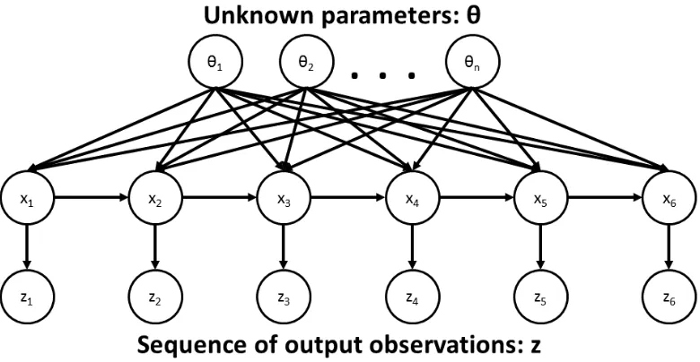
The statistical relationship between states and observations for the Bayesian state estimation problem is expressed using the graphical model in Figure 1.3.

(21)

[image:21.612.112.502.242.444.2]

Figure 1.2: Graphical Model of Bayesian Filtering/State Estimation

Figure 1.3: Graphical Model of Bayesian Parameter Estimation

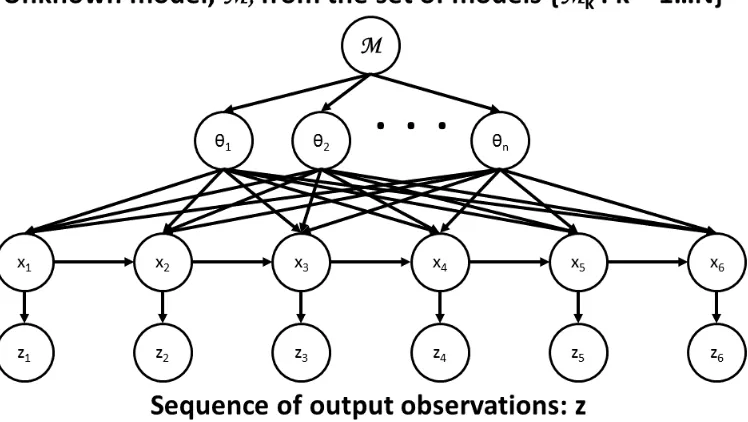
p(M | z1:k)=

p(z1:k | M)p(M) p(z1:k)

∝

∫

p(z1:k |θ1:n,M)p(θ1:n | M)dθ1:n

p(M)

(1.11)

The statistical relationship between parameters, states, and observations is expressed as a graphical model in Figure 1.4.

Applications of Bayesian Methods

(22)

[image:22.612.117.491.83.294.2]

Figure 1.4: Graphical Model of Bayesian Model Selection

practitioners to develop a better understanding of system modeling uncertainties, which can be integrated into the Bayesian framework to solve problems in uncertainty quantification, Bayesian optimization, and optimal experimental design. These tools are critical to robust system development, operation, and investigation,

Uncertainty quantification makes robust predictions about the future taking into account all sources of uncertainty [KO01; Chk+13; BT13; Naj09]. After solving a Bayesian inference problem, this updated understanding of the system model can be incorporated into robust predictions by marginalizing over the collective modelling uncertainty and other sources of uncertainty.

Bayesian optimal experimental design is a method to close the loop between data collection and inference by addressing the question of what experiment should be performed or measurement taken to best improve the estimate of some quantity of interest [CV95; HM13; KSG08; Bus+13]. Typically, Bayesian optimal experimental design takes the form of maximizing the expected information gain, also known as the relative Shannon entropy or the Kullback-Leibler divergence, between the prior and posterior given this potential data. This approach relies on the ability to solve the inverse problem to estimate the posterior distribution. This type of experimental design is critical for complex systems where data is often very expensive and there are complex relationships that constrain the identifiability of the posterior.

(23)

re-spect to very complicated black-box objective functions [BCD10; Sri+09], including functions with noise and uncertainty. This is done using the Bayesian framework. This method can then be used to design and optimize systems under uncertainty and explore the space of potential solutions by balancing an exploration and exploitation tradeoff.

Bayesian Inference Architecture for Dynamical Systems

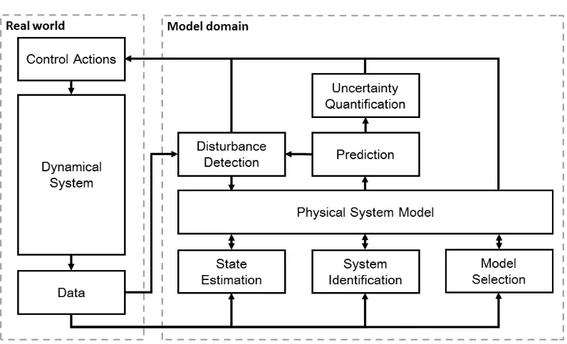
In order to efficiently integrate the Bayesian philosophy into the work of scientists and engineers, a general framework for inference problems for dynamical systems based upon theoretical models is needed. A conceptual approach to help formulate system level problems from the perspective of Bayesian inference is developed to do this in Figure 1.5. Typically, systems can be divided into processes that act on different temporal, spatial, and magnitude scales; therefore, learning and prediction algorithms should mirror these properties. By thinking about inference as a layered architecture, and utilizing this structure, inference can be performed quickly and flexibly.

On fast time scales, filtering methods are used for state estimation to determine the current operating state of the system. These methods are less flexible than full system identification estimation since they assume a system model but are very fast and can handel normal variations during operation. Then, by predicting the future distribution of responses for the system and comparing it to real observed data, large disturbances can quickly be detected so that appropriate actions can be taken to mitigate these events. This allows for greater flexibility in the detection of large, catastrophic disturbances, while still being fast. On slower time scales, as more data becomes available, the system model can be updated using system identification and model selection to identify disturbances or respond to gradual changes in the system. By allowing the model describing the system to be updated, the estimation architecture gains more flexibility. Using a fully Bayesian approach based on probability distributions, this architecture robustly combines inference, event detection, uncertainty quantification, and experimental design to have a closed loop approach to learning about a system’s behavior.

1.3 Markov Chain Monte Carlo Methods for Bayesian Inference

Solving Bayesian Inference Problems

(24)

[image:24.612.108.506.62.304.2]

Figure 1.5: A layered Bayesian approach for fast and flexible estimation and control.

analytical distribution. While approximate methods exist, they often have difficultly handling locally identifiable or unidentifiable problems [Bec10; Gel+14], where Bayesian methods are most needed. As a result, sampling methods are commonly used. The most common family of sampling methods is Markov Chain Monte Carlo (MCMC) [Bro+11], which creates a Markov chain defined by a transition rule, or kernel, whose stationary distribution is the desired posterior. In order to make estimates accurately, the samples must discretely capture the posterior distribution in a probabilistically appropriate way. Generating these samples makes MCMC computational intensive, as often thousands to millions of model evaluations are needed to fully populate the high probability content of a complex posterior. While, by the central limit theorem, the estimate quality for the mean of a finite-variance stochastic variable scales independently of the dimension given independent sam-ples, MCMC methods produce correlated samsam-ples, which can introduce poor high dimensional scaling. Many high dimensional problems where it is difficult to produce an efficient proposal distribution experience a “curse of dimensionality" because the sample correlation becomes very high. Thus, solving inference prob-lems using Bayesian methods is often prohibitively expensive because sampling high dimensional distributions efficiently is challenging.

(25)

E[g(θ) | D,M]=

∫

g(θ)p(θ | D,M)dθ≈ 1

N N Õ

i=1

g(θ_i) (1.12)

Assuming certain conditions hold, the quality of this estimate and its convergence can be assessed by the Markov chain central limit theorem [Gey11].

Markov Chain Monte Carlo

The basis for many MCMC methods is the Metropolis-Hastings algorithm, which produces a Markov chain with a desired stationary distribution, π(θ), by design-ing a transition kernel, K(θ0| θ), such that the Markov chain is ergodic and re-versible [Gey11; RC11]. Reversibility is a sufficient condition for the existence of a stationary distribution,π(θ), that satisfies the detailed-balance condition:

π(θ)K(θ0 |θ)= π(θ0)K(θ |θ0) (1.13)

This sufficient condition means that any transition kernelK(θ0| θ)may be chosen to maintain the stationary distributionπ(θ), as long as the reversibility condition (1.13) holds. Further, the composition of two kernels which have the same invariant distribution, π(θ), then also has π(θ) as its invariant distribution [Gey11]. This method can be used to create non reversible Markov chains with the correct stationary distribution out of a composition of reversible kernels.

α(θ0| θ)=min

1, π(θ0)Q(θ |θ0) π(θ)Q(θ0_| θ)

(1.14)

If the candidate is rejected, the current sample θ is repeated. This leads to the Metropolis-Hastings algorithm:

1. Initialize the stateθ1randomly, usually according to the prior, setn= 1

(26)

3. Accept or reject the candidate according to a sampled uniform variableζ on [0,1]:

θn+1=    

  

θ0

n+1 ζ ≤ α θ

0

n+1 | θn

θn ζ > α θ0_n₊₁ | θn

(1.15)

4. Incrementnand go to step 2

The evolution of the Markov chain according to the Metropolis-Hastings algorithm is illustrated in Figure 1.6. The resulting Markov chain has samples which are not independent, but correlated. Thus, the effective number of independent samples must be estimated to properly understand the convergence statistics. Based upon the Markov chain Central Limit Theorem, a standard method for judging the quality is the effective sample size (ESS) of the Markov chainθ1:N defined by

E SS[θ_1:N]= N

1+2ÍN_k₌₁ρk(θ1:N)

(1.16)

where ρk is the k lag autocorrelation function [DP11]. This provides a guide for

how to resample θ1:N to generate a set of ESS effectively independent samples

or how to incorporate the ESS into variance estimates. The effective sample size may be estimated for any function, E SS[g(θ_1:N)]. This gives useful convergence information for the function, which is particularly relevant when evaluating variance estimates. The quality of the variance estimate is based upon the ESS of the second order moment ofθ, not the ESS ofθitself.

The major challenge for the Metropolis-Hastings algorithm is designing an effective proposal distribution. The desired behavior of the Markov chain is for it to (1) converge quickly to the stationary distribution, that is, have a short burn-in time, and (2) have low correlation while sampling the stationary distribution. Optimal proposal distribution results only exist in simple cases [Ros+11; R+01].

Limitations of Metropolis-Hastings MCMC

(27)

Figure 1.6: Illustration of the evolution of a Markov chain for Metropolis-Hastings MCMC.

of finding and sampling it efficiently. Even when starting on the manifold, randomly sampling the region around it without detailed knowledge of that manifold will lead to low probability samples. Thus, if the proposal distribution is ill informed, very short steps are needed to ensure high acceptance rates, which leads to highly correlated samples. These types of distributions are common in inverse problems for complex dynamical systems where the data is not sufficiently rich to detangle the complex relationships produced by the dynamics leading to unidentifiable or only locally identifiable posteriors.

Further, even for simple distributions without complicated geometry, Metropolis-Hastings MCMC requires many model evaluations to produce an effective number of samples. Practitioners often run chains for hundreds of thousands or millions of iterations to ensure they have sufficiently uncorrelated their samples. Avoiding slow mixing by developing more efficient samplers is therefore critical for solving inference problems involving PDEs or ODEs where evaluating the forward model is computationally intensive.

(28)

has local information about its current state. Solving computationally intensive inverse problems, like those for complex dynamical systems, requires being able to exploit parallelism and adaptation based upon global information.

Several methods have been proposed to address this problem; however, no method has emerged as a general solution. Population based methods like Transitional MCMC (TMCMC) [CC07] and the Asymptotically Independent Markov Sam-pler (AIMS) [BZ13] work well for moderately high dimensional problems where a population of samples is able to capture the global structure of the posterior. Methods based upon exploiting local structure are also used, such as Adaptive MCMC [Ros+11] and HMC [Nea11]. Adaptive MCMC methods allow the pro-posal distribution to change slowly over time to better exploit the local posterior distribution geometry, while still maintaining the ergodicity of the Markov chain under some conditions. This adaptation enables Adaptive MCMC to work well for high dimensional problems. HMC is able to use the local gradient structure of the posterior distribution to gain high acceptance rates. This algorithm sam-ples along trajectories of almost constant energy, where the energy is defined as the joint probability of the posterior “potential energy" and a Gaussian momentum auxiliary variable or “kinetic energy" term. Riemannian Manifold HMC (RHMC) [GC11] further exploits local structure by making the kinetic energy position depen-dent [BS11]. The method introduced in [Ott+16] further extends HMC to infinite dimensional function spaces.

Contributions of this thesis

In Chapter 2, I discuss the Second-Order Langevin Monte Carlo sampler (SOL-MC) and its application to Bayesian inference. SOL-MC grew out of previous work which used the Second-Order Langevin stochastic differential equation (SDE) to approximately sample from probability distributions [TOM10; Tao11; MCF15]. Previous work also developed a Metropolized integrator, MAGLA, for this SDE [BO10; BV10] that maintains the correct invariant distribution, which we utilize. The results in this chapter are also found in [CB17]. My contribution in this work is to:

• Introduce SOL-MC for Bayesian inference

(29)

In Chapter 3, I explore the broad class of Sequential Tempered MCMC (ST-MCMC) algorithms which incorporate annealing, importance sampling, and MCMC to grad-ually transform a sample population from the prior to the posterior. Previous work on the development of these algorithms and their basic theory can be found in [CC07; DDJ06; MSB13]. My contribution in this work is to:

• Develop a theory to describe under what conditions learning is possible using ST-MCMC

• Introduce a feedback controller for the proposal distribution scaling during the Metropolis step to allow better tuning

• Introduce the Rank One Modified Metropolis Algorithm (ROMMA) to better enable scaling to high dimensions

In Chapter 4, I apply Bayesian methods to develop a learning architecture for power systems, specifically studying dynamic state estimation and fault detection and classification. This project grew out of work on fault classification done in [Wie+14] and further developed in our paper [Gar+15]. My contribution in this work is to:

• Introduce an integrated Bayesian state estimation, fault detection, fault clas-sification, and prediction architecture

• Develop a new implicit formulation of the Extended Kalman Filter for the state estimation of the differential algebraic equations describing the power system

• Formulate fault detection and classification as a Bayesian model selection problem

• Develop local and distributed methods for estimation on the power system to increase speed and robustness to disturbances

(30)

• Transform the forward model of the biosensor into a suitable probabilistic model for Bayesian inference

• Formulate the detection and identification of unknown inputs as a Bayesian inference problem

(31)

C h a p t e r 2

SECOND ORDER LANGEVIN MARKOV CHAIN MONTE

CARLO

In this chapter, we introduce the Second-Order Langevin Monte Carlo sampler, a MCMC algorithm which integrates many of the advantages of dynamical systems based sampling methods. The SOL-MC sampler is a based upon an auxiliary stochastic dynamical system, which enables us to study and optimize its perfor-mance using tools from the field of dynamical systems. We first provide motivation and discuss MCMC methods in general based upon auxiliary dynamical systems. Then we present a particular method based on the second-order Langevin stochastic differential equation to sample from a posterior distribution and show its relation-ship to the dynamical systems which underly other MCMC methods. Finally, we discuss the numerical implementation and metropolization of the SDE to ensure convergence to the correct posterior distribution, resulting in the final SOL-MC algorithm. Following the development of SOL-MC, we discuss tuning SOL-MC to optimize performance and present an example system identification problem to investigate SOL-MC under different conditions. Finally, we discuss some exten-sions of SOL-MC and compare these extenexten-sions to other dynamical systems based samplers using a simple test problem.

Much of the work presented here has appeared in:

[CB17] Thomas A Catanach and James L Beck. “Bayesian System Identifi-cation using Auxiliary Stochastic Dynamical Systems”. In: Interna-tional Journal of Non-Linear Mechanics (2017). doi: 10 . 1016 / j . ijnonlinmec.2017.03.012. url:https://doi.org/10.1016/ j.ijnonlinmec.2017.03.012.

2.1 Motivation

(32)

result, even though the candidate samples are far from the current sample, they will have high acceptance probability, thus reducing sample correlation. This is achieved by constructing a Hamiltonian dynamical system whose potential energy function is the negative log posterior probability density function (PDF), while the kinetic energy function is quadratic in the velocity coordinates of the auxiliary system, giving the corresponding momentum vector a Gaussian distribution independent of the position coordinates in the simplest setting where the mass matrix is constant. The marginal position distribution of this system is the desired parameter posterior. An application of HMC to Bayesian updating of high-dimensional dynamic systems is given in [CB09].

This auxiliary dynamical systems approach can be extended to stochastic dynamical systems, described by a stochastic differential equation (SDE) whose stationary distribution corresponds to the posterior of the Bayesian inference problem. These SDE approaches can not only be used in a standard MCMC framework, but can also be used to approximate the distribution without Metropolis steps [WT11; CFG14; MCF15]. SDEs are an active area of research, so there is a great opportunity to leverage these results to study the properties of these algorithms, such as work in infinite-dimensional spaces [Ott+16; DS13; Bes+11]. MCMC sampling based upon the damped second-order Langevin equation was originally introduced as a generalization of HMC for molecular dynamics by [Hor91]. Recently it has also been used as a sampler for Bayesian inference [TOM10; CFG14; Ott+16]. This SDE is an effective choice because it combines Hamiltonian dynamics with an Ornstein-Uhlenbeck process, which enables the state to both follow likely trajectories and to diffuse.

(33)

2.2 Dynamical Systems-based Samplers

Several dynamical systems-based methods for sampling arbitrary target probability distributions have been proposed, such as the Metropolis-adjusted Langevin Algo-rithm (MALA) [RS02], Hamiltonian/Hybrid Monte Carlo (HMC) [Dua+87; Nea11; GC11], and Stochastic Gradient MCMC (SG-MCMC) [WT11; CFG14; MCF15]. These methods combine a deterministic dynamic process, which encourages ex-ploration of high probability regions, with a method to inject noise, which enables diffusion and random sampling. The goal is to maximize convergence rate and minimize correlation while sampling the stationary probability distribution.

HMC begins by creating a Hamiltonian system whose position coordinates θ cor-respond to the model parameters in the Bayesian inference problem and whose momentum coordinates pare auxiliary variables added to embed the dynamics. A separable HamiltonianH(θ,p)is constructed where the potential energyV(θ)is the negative log of the target PDF, π(θ), and the kinetic energyT(p)is quadratic inp

with mass matrixM:

H(θ,p)=V(θ)+T(p)=−logπ(θ)+ 1 2p

T

M−1p (2.1)

The joint probability distributionΠ(θ,p)is then given by

Π(θ,p) ∝exp(−H(θ,p))= π(θ)exp

−1 2p

T M−1p

(2.2)

Notice thatphas a zero-mean Gaussian distribution with covarianceM.

(34)

[image:34.612.162.454.70.350.2]

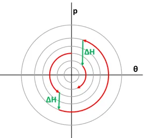
Figure 2.1: Illustration of the evolution of HMC for a 1D Gaussian posterior. The level sets of the Hamiltonian are seen in gray. The red trajectories illustrate the evolution of the system along a level set according to Hamiltonian dynamics. The green steps illustrate momentum resampling, which changes the level set.

The choice of the auxiliary mass matrix M is critical for creating a high efficiency algorithm since it guides the momentum re-sampling. This makes HMC sensitive to the auxiliary system parameter selection [BS11]. Alternatively, HMC can be extended to better adapt the momentum distribution to the local geometry through Riemannian Manifold HMC (RM-HMC) [GC11]. In RM-HMC, the fixed mass matrix M is replaced by a position dependent metricG(θ), which results in a new

Hamiltonian:

H(θ,p)=V(θ)+ 1

2log|G(θ) |+ 1 2p

T

G(θ)−1p (2.3)

(35)

a term proportional to the magnitude of local curvature, log|G(θ) |. Thus, when a trajectory transitions from a region of high curvature to low curvature, it gains kinetic energy so it will move faster through that region, enabling it to sample farther from the initial point. Further, the metric orients the momentum distribution to align with the curvature of the manifolds, so trajectories favor moving along the dominant directions of the manifold. Several methods have been presented for choosingG(θ),

based upon the Hessian. Since the metricG(θ)must be positive definite, the Hessian cannot be used directly. Instead, functions of the Hessian like the non-degenerate Fisher information matrix [GC11] and the SoftAbs metric [Bet13] are used.

While HMC uses momentum resampling then deterministic dynamics to propose candidate samples, SG-MCMC and MALA create a discrete-time approximation to an underlying stochastic differential equation. A Metropolis correction can then be applied to the discretization of this SDE to ensure it has the desired posterior as its stationary distribution. MALA is based upon the Metropolis-Hastings algorithm, but incorporates a Langevin diffusion into the proposal distribution for candidateθ0 [RS02], which typically gives it a shorter burn-in period to the posterior distribution than Metropolis-Hastings because the gradient term directs exploration:

θ0₌ _θ₊

hM∇logπ(θ)+ √

2hMξ (2.4)

Mis a preconditioning matrix,hthe auxiliary time step,ξhas a standard multivariate Gaussian distribution, and

√

M for a positive definite matrix M indicates a matrix square root. In general, the choice of diffusion used to sample the distributionπ(θ) is not unique. A broad class of possible diffusions if presented in [RS02].

Similarly, SG-MCMC creates a SDE whose marginal stationary distribution can be any posterior π(θ). This leads to a general framework for constructing a Markov process [MCF15]:

dz= f (z)dt+p2D(z)dW(t) (2.5)

The states,z, of the SDE are a combination of the variablesθand additional auxiliary variables. Within this framework, the SG-MCMC method is defined by the choice of a diffusionD(z)and drift term f (z). This may be done by choosing a Hamiltonian

H(z), positive-semidefinte diffusion matrixD(z), and skew-symmetric curl matrix

(36)

f (z)= − [D(z)+Q(z)] ∇H(z)+Γ(z)

Γ(z)_i =

d Õ

j=1

∂ ∂zj

Di j(z)+Qi j(z) (2.6)

with the distribution onzthen given by

π(z) ∝exp(−H(z)) (2.7)

2.3 SOL-MC Sampler

Second Order Langevin SDE

Similar to the methods in Section 2.2 we choose an underlying auxiliary dynamical system to derive the second-order Langevin (SOL) Stochastic Differential Equation and define our SOL-MC sampler. To do this, we use the described framework above from [MCF15]. We choose the Euclidean Hamiltonian (2.1), and the diffusion matrix and the curl matrix are taken as:

D(z)=

"

0 0

0 C(z)

#

(2.8)

Q(z)=

"

0 −I

I 0

#

(2.9)

These choices can be interpreted as creating an SDE that combines Hamiltonian dynamics with an Ornstein-Uhlenbeck (OU) process. Solving (2.6) using these choices forH(θ,p),D, andQyields the second-order Langevin or inertial Langevin SDE:

dθ = M−1pdt

dp=−∇V(θ)dt−C M−1pdt+√2CdW (2.10)

It was shown much earlier than [TOM10] by [Cau63] that this SDE, which models a viscously-damped nonlinear elastic dynamic system excited by white noise, has a stationary distribution defined by the Boltzmann-Gibbs distribution:

Π(θ,p) ∝exp[−H(θ,p)]=exp

−1 2p

T

M−1p−V(θ)

(37)

Figure 2.2: Illustration of the trade-off of choosing the damping. If there is very little damping, Hamiltonian dynamics dominate resulting in a highly correlated trajectory that can quickly explore the space. If there is high damping, the OU process dominates which results in less coherent evolution but also less exploration of the space. For optimal damping, the trajectories balances the drift and diffusion processes to explore the space without excessive correlation.

The HamiltonianH(θ,p)is the sum of a quadratic kinetic energy term and a pseudo potential energy termV(θ):

V(θ)=−logπ(θ) (2.12)

This SDE can be used to sample from an arbitrary PDF π(θ). To accelerate the convergence of the SDE to the appropriate stationary distribution π(θ), [TOM10] introduced a diffusion term using the damping matrixC(θ)in (2.10). The choice ofC(θ) determines whether the Hamiltonian dynamics or the diffusive dynamics dominate the trajectory. This trade-off is illustrated by Figure 2.2. The optimal choice of damping is considered in a later sub-section. Alternatively, if we choose the Hamiltonian (2.3), instead of (2.1), as the basis for our sampler, then we get a Riemannian formulation of the SOL SDE sampler, SOL-RMC.

Numerical Integration

(38)

Hamil-ton’s equation is approximated using a symplectic integrator, while the solution to the Ornstein-Uhlenbeck equation is solved exactly since it is a linear equation.

The GLA solves this SDE using Strang-Type Splitting:

(θk+1,pk+1)=ψtk+h,tk+h/2◦Θh◦ψtk+h/2,tk(θk,pk) (2.13)

This is a composition of two integrators: ψtk+h/2,tk (θ,p), which integrates the

Ornstein-Uhlenbeck process exactly from tk to tk + h/2, a half a time step, and Θh(θ,p), which approximately integrates the Hamiltonian system forward by a full

time steph:

ˆ

pn =exp

−h

2CnM

−1_pn₊q _I₋_exp ₋_hCn_M−1 _M_ξˆ_n

p1n/2= pnˆ − h

2∇V(θn) θn+1= θn+hM−1p1

/2 n

¯

pn₊1= p1

/2

n −

h

2∇V(θn+1)

pn₊1 =exp

−h

2Cn+1M

−1_pn_¯

+1+ q

I−exp −hCn₊1M−1 Mξn

(2.14)

We choose this 2nd-order GLA integrator because the 1st-order GLA integrator that is used in [TOM10] is not reversible and thus cannot be metropolized. It combines the exact integrator for the Ornstein-Uhlenbeck process with a symplectic Stőrmer-Verlet method for the Hamiltonian equation [BO10]. While this method is also not directly reversible, it is reversible when combined with a momentum flip. This momentum flip makes it similar to other metropolized dynamics based samplers such as HMC [BV10; Dua+87; Hor91].

Metropolization

The discretization in (2.14) for the SOL SDE in (2.10) introduces numerical errors so that (2.14) need not have the target stationary distribution. In order to ensure that the sampler exactly samples from the correct targetπ(θ), we add a Metropolis step after each integration time step. A metropolized formulation of a general GLA integrator for the inertial Langevin equation is introduced in [BV10] as the Metropolis Adjusted Geometric Langevin Algorithm (MAGLA). This metropolized formulations builds upon the original work of [Dua+87; Hor91]. The proposal(θ_n,pn) → θ∗

n+1,p

∗

n+1

(39)

the GLA integration algorithm (2.14). The Hamiltonian dynamicsΘhare reversible

when combined with a momentum flip. This reversibility means that

θ∗

n+1,p

∗

n+1

=Θh(θn,pn)

(θn,−pn)=Θh θ_n∗₊₁,−p∗_n₊₁

(2.15)

The Metropolis acceptance step is defined by

(θ_n₊₁,pn₊1)=        θ∗

n+1,p

∗

n+1

, ifζn < α θn,pn, θ_n∗₊₁,p∗_n₊₁

(θn,−pn), otherwise

(2.16)

where ζn is a sampled uniform variable on[0,1] and the momentum is flipped if

the candidate is rejected to maintain reversibility. The acceptance probability α in (2.16) is given by the Metropolis-Hastings algorithm (1.14):

α θn,pn, θ∗_n₊₁,p∗_n₊₁ =min       

1, Q θn,−pn | θ

∗

n+1,p

∗

n+1

Π θ∗_n₊₁,p∗_n₊₁

Q

θ∗

n+1,−p

∗

n+1 | θn,pn

Π(θ_n,pn)

       (2.17)

where the posteriorΠ(θ,p)is defined by (2.11) while the ratio of the proposal PDFs

Qis defined by

Q(θn,−pn|θ∗_n₊₁,p_n∗₊₁)π(θ∗_n₊₁,p∗_n₊₁)

Q(θ∗_n₊₁,−p∗_n₊₁|θ_n,pn)π(θn,pn) =exp

−∆E θn, θ_n∗₊₁

∆E θn, θ_n∗₊₁ =

1

2D2Ld θn, θ

∗

n+1,h T

M−1D2Ld θn, θ∗_n₊₁,h +V θ∗_n₊₁

−1

2D1Ld θn, θ

∗

n+1,h T

M−1D1Ld θn, θ∗_n₊₁,h −V(θn)

(2.18)

While [BV10] show this result when the friction coefficient C is constant, it still holds whenCis a function ofθ. In (2.18),Ld(θn, θn+1,h)is the discrete Lagrangian

which defines the symplectic integration scheme. For the 2nd-order GLA, the derivatives of the discrete Lagrangian are

D1Ld θn, θ∗_n₊₁,h =− M

θ∗

n+1−θn

h −

h

2∇V(θn)

D2Ld θn, θ∗_n₊₁,h =M

θ∗

n+1−θn

h −

h

2∇V θ

∗

n+1

(40)

Optimization and Tuning of SOL-MC

When implementing SOL-MC prescribed by (2.10), we have the freedom to choose the auxiliary mass matrix M and damping matrixC of the SDE. While designing the sampler, our goal is to speed up convergence to the stationary distribution and minimize correlations once the stationary distribution is reached to keep the effective sample size, ESS in (1.16), as large as possible. The first step toward choosing these parameters is to study the behavior of SOL-MC when sampling a Gaussian distribution, because the SDE for sampling the Gaussian can be solved analytically.

Gaussian Linear System

When the target distribution is a zero-mean Gaussian, it is straightforward to prove several optimality results. The Hamiltonian for this system is quadratic:

H(θ,p)= 1

2p T

M−1p+ 1₂θTGθ (2.20)

Thus, the SDE reduces to a stochastic linear system, which yields the continuous time dynamical system of the form zÛ=Az+bw:

"

Û θ Û

p #

=

"

0 M−1

−G −CM−1 # "

θ

p #

+

"

0

p

2C(θ) #

w (2.21)

Mass Matrix

The Gaussian potential in the Hamiltonian (2.20) has constant curvature, where

G(θ) = G = Σ−1 0. As discussed in Section 2.2 for HMC and RM-HMC, by choosing M, the mass matrix for the auxiliary system, to be G, the momentum distribution will align with the dominate directions of the Gaussian distribution. This reduces sample correlation. For the pseudo potential energy of a general posterior distribution, we locally approximate the system with a quadratic potential by taking the Hessian matrix of the potential,∂2_∂θV(₂θ). This a real symmetric matrix so it has a spectral decomposition in terms of the real eigenvaluesΛand orthonormal eigenvectorsQ:

H(θ)=∂ 2_V_(θ)

∂θ2

=QΛQT

(41)

The Hessian is not guaranteed to be positive definite, and so it must be transformed to be a suitable choice for M. We choose to use the SotfAbs metric [Bet13] ˜H. This choice smoothly transforms the small and negative eigenvalues of the matrixH

using a smoothing parameter. Small eigenvalues are mapped close to and large negative eigenvaluesλare mapped to−λ. The transformation is

M=H˜ (θ)

=QΛcoth−1ΛQT

(2.23)

When choosing, the smaller the, the flatter the quadratic estimate of the potential can be thus enabling the sampler to take larger steps in the flat directions, making generally small preferred. However, two factors keep from becoming too small. First, the long steps will cause numerical integration to be less accurate particularly when the problem is non-linear. Second, the prior distribution often introduces bounds for parameter values. Thus, if the posterior is flat, but bounded, and is small, the trajectories will often overshoot the boundary, causing a high rejection rate.

Since we are not concerned with maintaining detailed-balance while the SDE is converging to the stationary distribution during the burn-in period, we can adapt

M to reflect the local geometry via (2.23). Once we judge that we have reached the stationary distribution based upon the statistics of multiple chains,Mis fixed to reflect the local curvature of the stationary distribution.

Damping Matrix

For the linear stochastic dynamical system (2.21) withM= I, the dampingC(θ)is chosen in [TOM10] by minimizing the maximum real part of the eigenvalues of the dynamics matrixA. This choice corresponds to critical damping, which maximizes the convergence to the stationary distribution and thus minimizes the burn-in period. They find thatC(θ) = 2√G. More generally, it can be shown that whenM, C, G

are simultaneously diagonalizable,C(θ)=2√GM. The eigenvalues ofAin (2.21) are given by

det(A−λI)=det

λCM−1+λ2+M−1G

=detλΛCΛ−_M1+λ2+Λ−_M1ΛG

=0

(42)

whereΛM,ΛC, andΛGare the eigenvalues ofM,C, andG, respectively, expressed

as diagonal matrices. Since the system is now diagonal, we can see that in general the eigenvaluesλi take the form of

λ=− λC,i 2λM,i

± 1 2

v u tλ2

C,i

λ2 M,i

−4λG,i λM,i

(2.25)

The largest eigenvalue is then minimized whenλC,i =2 p_λ

G,iλM,isoC(θ)=2

√

GM. For a more general case, whenMandGdo not necessarily commute, this choice of parameters will not necessarily be positive definite. Thus, we choose the positive definite matrix 2

√

M1/2_GM1/2 _{for a general}_M_and_G_{. When the dynamic system}

is non-linear, we linearize it by taking the Hessian matrix of the potential, ∂2_∂θV(2θ).

We then transform this using (2.23) into a positive definite matrix, ˜H, to capture the curvature of the potential surface, giving it the ability to adapt to the local geometry. This is the same as locally fitting a Gaussian distribution to the posterior and using that linear system to design the damping. Ultimately this yields

C(θ)=2

q

M1/2_H˜ (θ)M1/2 _(2.26)

Convergence and Correlations

As shown in the previous section, minimizing the largest eigenvalue of the linear stochastic dynamical system (2.21), whenMandGcommute, maximizes the conver-gence rate since the system is critically damped. Furthermore, this also minimizes the autocorrelation function for this system. The general stochastic linear system

Û

z=Az+bwhas the solution:

z(t)=exp[At]z(0)+

∫ t

0

exp[A(t−s)]bdw(s) (2.27)

Let the dynamical system be converged to its stationary distribution and z(0) be its state. Then assuming the stationary distribution is a zero-mean Gaussian, with covarianceΣ, the covariances between z(t)andz(0)is:

cov[z(t),z(0)]=exp[At]Σ (2.28)

(43)

coordinate system individually. The dynamics of each of these 2D systems is de-scribed in [Per13]. The matrix exponential, exp[At], decays at a rate proportional to exp(Re[λ]t)and has a known form which depends on whether the eigenvalues are both real, both complex, or identical. Minimizing the maximum real part of the eigenvalues in (2.25) causes this decay rate to be fastest, which minimizes the autocorrelation over the trajectory. Thus the effective sample size of the MCMC sampler defined by this SDE will be highest.

Computational Considerations

Dynamical systems based sampling methods require taking derivatives of the likeli-hood function. Taking the gradient is unavoidable since it produces the underlying dynamics. Computing the Hessian is useful for capturing the correlation structure and the appropriate length scales. Traditional techniques like symbolic derivative solvers or finite differences do not scale, are computationally intensive, and often imprecise. Automatic Differentiation (AD) presents an alternative approach that typically outperforms these traditional methods. AD analyzes code as it compiles and computes the derivative based upon the underlying elementary operations being executed on the machine level using the chain rule. Since it takes derivatives of the computer code itself, it can take derivatives of much more complicated likelihood functions than symbolic methods. While AD libraries have been developed for a variety of languages, Julia, a language specifically designed for scientific computing is especially powerful [Bez+12; RLP16]. Julia looks like a scripting language but is “just-in-time” compiled, thus giving it the speed of a compiled language like C. We choose Julia for implementing SOL-MC.

As an example, for the shear building model in the next section, the likelihood function takes approximately 0.2 second to evaluate and has up to 12 parameters. Using AD, the gradient computation takes 1.8 seconds and the Hessian takes around 9.3 seconds. When using finite differences, the gradient takes 5.8 seconds and the Hessian 150 seconds. Thus we see significant computational cost savings.

2.4 System Identification Example

Hysteretic Structure Model

(44)

model can produce globally identifiable or unidentifiable cases. For the globally identifiable case, we show that SOL-MC is able to effectively find and sample the posterior efficiently. For the unidentifiable case, we show that SOL-MC can still sample the posterior, but samples with less efficiency than in the globally identifiable case.

System Identification Problem

We consider the problem of identifying unknown parameters for the three-story Masing shear building model where the building is excited by earthquake ground motion as in [MB08]. We used ten seconds from the Sylmar ground motion record at the Olive View Hospital parking lot recorded during the 1994 Northridge earthquake and available from the Strong-Motion Virtual Data Center [Eng]. This acceleration time history is sampled at a 50 Hz. The mass distribution for the structure can be estimated from structural drawings much more accurately than the other structural model parameters, and so we assume that the mass of each story is known and it is 1.25×105kg. The pseudo-static influence vector b is known to be[1 1 1]T. The small-amplitude inter-story stiffnessKiis unknown but has a true value of 2.5×108 N/m for each story when simulating the synthetic response data. The ultimate strengthru,i is unknown for each story, but has an actual value of 1.75×106N. The

smoothness parameterαi is also unknown, but it is assumed to have the same value

αfor each story. Its true value is 4. We assume that the viscous damping matrixC

takes the form of a Rayleigh damping matrix:

C= cmM+ckK (2.29)

where the coefficients are unknown, but have true values of 0.293 for cm and 2.64×10−4forck.

The output y(t) = xÜ(t)+ν(t)is the acceleration of each story sampled at 50 Hz, yielding 500 samples in the trajectory for each of the three stories. The output is subject to Gaussian additive noise,ν(t), with mean zero and standard deviationσ. The value ofσis unknown, but has a true value of 0.5 m/s2. Ultimately, this yields a likelihood function for the output dataD of the form:

p(D | θ, σ)= 2πσ2 −_{Nd Nt}

2

exp

"

− 1 2σ2

Nd

Õ

i=1 Nt

Õ

t=1

y(_ti)(θ) −yˆ_t(i)

2 #

(45)

[image:45.612.68.553.59.330.2]

Figure 2.3: Position and potential energy trajectories of the four chains.

where the ten unknown parameters are θ = k1,k2,k3,cm,ck,ru,1,ru,2,ru,3, α, σ T

, ˆ

y_t(i) is the measured output at time step t of story i and y(_ti)(θ) is the simulated expected output given parametersθ.

The prior distributions on the parameters are chosen as follows: Kihas a log normal prior with logarithmic mean log 2.5×108and logarithmic standard deviation 0.5;

ru,ialso has a log normal prior with logarithmic mean log 2.5×108

and logarithmic standard deviation 0.5;αhas a log normal prior with logarithmic mean log(4.0)and logarithmic standard deviation 0.5;σ2_{has a uniformly distributed prior between 0}

and 3;cmhas a uniformly distributed prior between 0 and 1.5; andckhas a uniformly distributed prior between 0 and 1.5×10−3.

(46)

Results: Globally Identifiable Case

We began by simulating several Markov chains to estimate when the SDE reached stationary state. During this initial burn-in phase, 300 steps were simulated where the SDE was solved without Metropolis correction to speed up convergence. The steady state can be identified once the likelihood function stops changing significantly and the chains appear to be sampling from the same region. Four chains were selected based upon their posterior likelihood and they were used to simulate 2000 samples from the posterior using the metropolized sampler. The trajectory of the samples and the log posterior can be seen in Figure 2.3. We see that they converge to the stationary distribution in under 300 iterations and then begin sampling from it. The burn-in period was determined by inspecting the convergence of the log posterior function for the chains before the SDE is metropolized. During the burn-in period, the time step was set to 0.1 and the mass matrixMwas adapted to the local geometry. Once the burn-in period ended, the time step was set to 1.0 and the mass matrix fixed to ensure that the chain had the correct stationary distribution for the sampling. The potential surface in this example is generally very non-smooth, and so a smaller time step is needed to converge faster to the high probability manifold. Once the trajectory finds the high probability manifold, a larger step can be taken since it is typically much smoother.

The trajectories of many sample chains during a burn-in period can be seen in Figures 2.4 and 2.5. For the projection onto the σ2 and αplane given in Figure 2.4, we see that the trajectories generally converge to the same funnel like path as they move toward the stationary distribution at the bottom near (1,1). At early time steps, the trajectories increase the measurement varianceσ2since the data fit is so poor. Asσ2becomes very large, this effectively anneals the problem, allowing the trajectory to explore more space without getting stuck in a local minimum. As the data fit becomes better,σ2decreases constraining the trajectories, and forces them to converge to the high probability manifold. This works well since the model is globally identifiable.

In contrast, Figure 2.5 shows the projection onto theσ2andru,3plane, where there is