Softcodes of Parallel Processing Milne’s Device via
Exponentially Fitted Method for Valuating Special
ODEs
J. G. Oghonyon, Member, IAENG, M. R. Odekunle, A. O. Adesanya, O. F. Imaga Abstract- The idea of technological computing has immensely
assisted to enhance accuracy and maximize computed errors involving computational math. Softcodes computer programme is guided towards supplying comfortable computation, proficiency and faster results at all times. The objective of this study will be to devise softcodes of parallel processing Milne’s device (SPPMD) via exponentially fitted method for valuating special ordinary differential equations. This is established through collocation and interpolation of the exponentially fitted method. Dissecting (SPPMD) produces the principal local truncation error (PLTE) after expressing the order of SPPMD leading to the boundary of convergence. Some selected examples of special ODEs were tested to show the efficiency and accuracy of (SPPMD) at different boundary of convergence. The finished results exist with the aid of (SPPMD). Computed results show that the (SPPMD) is more proficient compare to subsisting methods in terms of the work out max errors at all levels.
Index Terms- Softcodes, exponentially fitted method, boundary of convergence, Principal local truncation errors
I. INTRODUCTION
Several computational methods for the direct consolidation of (1) exist and subsequently, authors have not been able to utilize the peculiar info concerning special ODEs. For instance, scholars will not take into consideration the vibrating or decomposing behavioral attributes of the exact solution. Thus, SPPMD is consider as one of the most effective technic for valuating special ODEs. See [15]. This research study sees special ODEs owning an exceptional character of the approximative solution been situated ahead of time. Such special problem is of the class [10]-[11], [14], [19], [26]
Manuscript submitted March 30, 2018; revised for submission April 7, 2018. This work was supported by Covenant University Centre for Research, Innovation and Discovery (CUCRID, Ota, Ogun State, Nigeria.
J. G. Oghonyon, Department of Mathematics, College of Science and Technology, Covenant University, P.M.B. 1023, Ota, Ogun State, Nigeria (corresponding author phone no.: +234-8139724200; [email protected]).
M. R. Odekunle, Department of Mathematics, Modibbo Adama University OF Technology, Yola, Nigeria
O. A. Adesanya, Department of Mathematics, Modibbo Adama University of Technology, Yola, Nigeria ([email protected]).
I. F. Imaga, Department of Mathematics, College of Science and Technology, Covenant University, P. M. B. 1023, Ota, Ogun State, Nigeria ([email protected]).
(1)
with vibrating exact solutions, where , is the proportion of the physical organization and . See [27], [34].
Equation (1) possesses majorly alternating, increasing and decomposing solutions that are widely known in numerous areas, these includes, ambiance, biological sciences, Newtonian mechanics, celestial bodies/universe, quanta theory, control theory and electrical circuit. Technological computing of distinct technics has been laid down by exponentially fitted method with recognized frequence and having solution beforehand abounds in literatures. Observe [4]-[5], [14], [19], [24] is particularly reserve. Scholarly persons have projected and implemented (1) to give the sought after result. See [27], [35]. However, [26]-[28] carried out all math calculations employing electronic computer programming code in Matlab format. On another occasion, [10]-[11], [17], [29]-[30]concluded math application using a composed encrypt in Mathematica 10. 0 to showcase the efficiency and accuracy of the technics. However, [9] executed all numeric computations on a PC computing machine device initiated by running PYTHON. Nevertheless, several shortcomings were noticed from the bookmen’s contribution listed supra. This admits; applying a set step size and lack of suit step size, lack of boundary of convergence to insure convergence of the method and cumbersome computation without error control. The motivation of this study stems from the need to design an exceptional SPPMD with known frequence of one as seen in [23], [34] thereby yielding better computed max errors at the least boundary of convergence.
From the gaps enlisted earlier, this research study apart from demonstrating the use of SPPMD comes with some computational benefits such as designing suitable step size, varying the step size, deciding the boundary of convergence to ascertain convergence and maximize error control. Hence, this constitute the primary objective of SPPMD as computing technics which is suitable to valuate vibrating problems. See [7], [12]-[13], [19]-[20], [32]-[33].
Theorem (Weierstrass Approximation Theorem)
Let be continuous and periodic. Then for each
, there exists a trigonometric polynomial
such that for all .
polynomial such that in a uniform manner on . See [8].
The residuary of this research study is as complies: in Subsection 2 SPPMD of Materials and Methods; in Subsection 3 Examples of Vibrating Problems; in Subsection 4 Computational Results and Discussion; in Subsection 5 Conclusion as cited [3], [32]-[33].
II. MATERIALS AND METHODS
Under this subsection, the objective to be attained will be to invent SPPMD. Parallel processing Milne’s device is a conjugation of parallel processing predictor scheme (PPPS) and parallel processing corrector scheme (PPCS) of ilk order. This pair is defined as
, (2)
. (3)
Par (2) and (3) gives the SPPMD with , containing characteristics that bank on suited step size, changing step size and frequence. Mentioning that is the
numeric estimate to the precise solutions i.e.
, and owning
. In order to arrive at par (2) and (3), the exponentially fitted method is employed in concert with the collocating /interpolating scheme to estimate the precise solution on time interval of for PPPS. Again, PPCS utilizes for
PPCS via the interpolating subprogram of the type (4)
. (4)
Rewriting (4) give birth to the softcodes of exponentially fitted method (SEFM) of the form
, (5)
since w is always given, and are unchanging parameters needed to ascertain in a particular manner. Presuming the condition that equation (5) matches the precise solution at some picked out interval to give the approximation as
, . (6)
Demanding that the interpolating function (6) gratifies par (1)
at the points
to bring forth the coming estimation of
PPPS as
(7) while PPCS is stated as
(8)
Uniting the estimation of (6), (7) and (8) will produce the four-fold systems of equation in Au=b pattern.
, (9)
, (10)
Working out the systems of equation will develop the softcodes of PPPS and PPCS for solving the systems of equation. Finding and subbing the measures of into (5) will generate the continuous SPPMD for PPPS and PPCS as
. (12)
Valuating the continuous PPPS and PPCS (11) and (12) at some selected points of will bring forth the
PPPS and PPPCS as
, (13)
(14)
where is the known frequence, and
are unchanging constants. Find [1]-[2], [13], [26]-[30], [32]-[33]for more items.
Inventing the convergence boundary of SPPMD
To propel the SPPMD, the PPPS and
PPCS are processed as PPPS-PPCS pair possessing the ilk order. A compendium of [7], [12]-[13], [19]-[20], [32]-[33] shows that it is executable to look for the approximate of principal local truncation error of the PPPS-PPPS pair in absence of calculating higher differential constants of .
Make bold that , where and establishes the order of the PPPS and PPCS. Straightaway, for a scheme of order , the investigation of PPPS will give birth to the principal local truncation errors as
(15)
.
A like computing analysis of PPCS will generate the principal local truncation errors as
(16)
,
where and are in existent as a separate entity of the step-size h and behave as the precise solution to the differential constant fulfiliing the starting pre-condition . See [7], [12]-[13], [19]-[20], [32]-[33] for more info.
To advance, the pre-condition is set small for h valuates to be attained as
, (17)
and executing the SPPMD relies immediately on this precondition put forward by (17).
Further simplification of the principal local truncation errors of (15) and (16) as well as dropping off terms of degree
, it gets well to achieve the computation of the
principal local truncation errors of SPPMD as
(18)
.
Citing the statements that , and
are acknowledged as PPPS and PPCS estimates brought forth by the SPPMD of order p, while
,
and
are distinctly named the principal local
truncation errors. and are the boundaries of convergence of SPPMD.
discontinue the final results of the iterative process or repeat the successive process with a smaller varying step size. The procedure is truly acceptable on the basis of a try out test evaluation as defined by (18). Check [7], [12]-[13], [19]-[20], [32]-[33] for more details.
III. NUMERICAL EXAMPLES
Two problems are studied and solve employing SPPMD at distinct boundaries of convergence such as , ,
and . See [23], [34] for more details. A softcodes
founded on SPPMD is composed applying computing software package. This SPPMD is carried out in a parallel
processing style as prescribed by SPPMD. See appendix.
Problem 1: Consider the initial value ODE
, .
Exact Solution: .
Problem 2: Consider the nonlinear Duffing equation:
, . Exact Solution: .
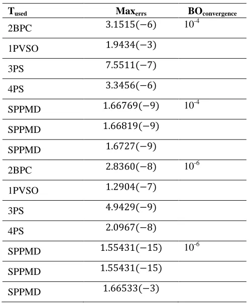
IV. RESULTS AND DISCUSSION
[image:4.612.315.563.414.731.2]This subsection introduces the softcodes of the computational results executed employing the SPPMD. The finalized output supplied were achieved with the assistance of Mathematica 9 kernel to show-case the efficiency and preciseness. See [1]-[2].
Table 1 of problem 1
Tused Maxerrs BOconvergence
2BPC 10-4
1PVSO
3PS
4PS
SPPMD 10-4
SPPMD
SPPMD
2BPC 10-6
1PVSO
3PS
4PS
SPPMD 10-6
SPPMD
SPPMD
Tused Maxerrs BOconvergence
2BPC 10
-8
1PVSO
3PS
4PS
SPPMD 10-8
SPPMD
SPPMD
2BPC 10-10
1PVSO
3PS
4PS
SPPMD 10-10
SPPMD
[image:4.612.48.297.424.726.2]SPPMD
Table 2 of problem 2
Tused Maxerrs BOconvergence
2BPC 10-4
1PVSO
SPPMD 10
-4
SPPMD
SPPMD
2BPC 10-6
1PVSO
SPPMD 10-6
SPPMD
SPPMD
2BPC 10-8
1PVSO
SPPMD 10-8
SPPMD
Tused Maxerrs BOconvergence
2BPC 10
-10
1PVSO
SPPMD 10-10
SPPMD
SPPMD
SPPMD: errors in SPPMD (Softcodes of parallel processing Milne’s device) for tested problems 1 and 2.
Tused: technic used.
Maxerrs: magnitude of the maximum errors of SPPMD.
: boundary of convergence.
2BPC: error in 2BPC (implementation of the two point predictor-corrector block method using variable step size) for tested problem 1 and 2. See [23]. 1PVSO: errors in 1PVSO (implementation of the one point method variable step size and order using the integration coefficients. See [23].
3PS: errors in 3PS (the implementation of the three-step implicit block method for tested problem 1. See [34].
4PS: errors in 4PS (the implementation of the four-step implicit block method for tested problem 1. See [34].
A composed step by step technic that will enforce the SPPMD implementation and valuation of the maximum errors is been prescribed below as follows:
Stride 1: Choose the step size for h.
Stride 2: The order of the parallel processing predictor-corrector pair must be the alike.
Stride 3: The stride measure of the parallel processing Predictor method must be one stride above the parallel processing corrector method.
Stride 4: Define the boundary of convergence of the SPPMD. Stride 5: Insert the SPPMD in any computing software package.
Stride 6: Adopt single stride technic to prime if necessary, if not, avoid stride 6 and move on to stride 7.
Stride 7: Carried out the implementation of SSPMD in computing software package.
Stride 8: If stride 7 is discontinued due to h value and boundary of convergence, adopt this new rule of generator stated below to find the true value of length h to achieve convergence, otherwise move on to stride 9.
.
Stride 9: Valuate the magnitude of the maximum errors after the boundary of convergence is satisfied.
Stride 10: Put into writing the magnitude of the maximum errors. See [32].
V. CONCLUSION
The computed terminal outputs shown in Table 1 and Table 2 demonstrates the SPPMD is attained with the aid of the boundary of convergence, suited and varying stride size. This boundary of convergence helps to check whether the looping is allowed or disallowed. Therefore, establishes the efficiency of the SPPMD to obtain better maximum errors compare to 2BPC, 1PVSO, 3PS and 4PS in the least boundary of convergence of , , , and as cited
[23], [34]. For this reason, it will satisfactory to resolve that the SPPMD is effective for computing special problem of frequence one as against [23], [34]. Further work will be to apply trigonometrically fitted parallel processing Milne’s device on first order ODEs.
APPENDIX
The SPPMD for solving problem 1 and 2 is seen infra. g[t_]=Exp[-t]
w=1
h= given value, x[n]=given starting value t=given value
g[1]=g[0]+h(g'[0])+(h^2/2)g''[0]+(h^3/6)g'''[0]+(h^4/24)g''''[0] g[2]=g[1]+h(g'[x[n]])+(h^2/2)g''[x[n]]+(h^3/6)g'''[x[n]]+(h^4/24)g''''[ x[n]]
g[3]=g[2]+h(g'[x[n]+h])+(h^2/2)g''[x[n]+h]+(h^3/6)g'''[x[n]+h]+(h^4 /24)g''''[x[n]+h]
g[4]=g[3]+h(g'[x[n]+2h])+(h^2/2)g''[x[n]+2h]+(h^3/6)g'''[x[n]+2h]+( h^4/24)g''''[x[n]+2h]
g[5]=g[4]+h(g'[x[n]+3h])+(h^2/2)g''[x[n]+3h]+(h^3/6)g'''[x[n]+3h]+( h^4/24)g''''[x[n]+3h]
t=x[n]+2h
g[4]=g[3]+h((-(6+3w-37w^2)/(6w^2))g'[t-x[n]]+(-19/3+3/w)g'[t-x[n]+h]-(-(6+3w-13w^2)/(6w^2))g'[t-x[n]+2h])
t=x[n]+4h
g[6]=g[4]+h((155/12+7/w^3-2/w^2-2/w)g'[t-x[n]]+(-46/3- 14/w^3+4/w^2+4/w)g'[t-x[n]+h]+(65/12+7/w^3-2/w^2-2/w)g'[t-x[n]+2h])
t=x[n]+6h
g[8]=g[5]+h((133/6+26/w^3-3/w^2-9/(2w))g'[t-x[n]]+(-85/3- 52/w^3+6/w^2+9/w)g'[t-x[n]+h]+(61/6+26/w^3-3/w^2-9/(2w))g'[t-x[n]+2h])
t=x[n]+5h
g[7]=g[6]+h((-(6+3w-37w^2)/(6w^2))g'[t-x[n]]+(-19/3+3/w)g'[t-x[n]+h]-(-(6+3w-13w^2)/(6w^2))g'[t-x[n]+2h])
t=x[n]+7h
g[9]=g[7]+h((155/12+7/w^3-2/w^2-2/w)g'[t-x[n]]+(-46/3- 14/w^3+4/w^2+4/w)g'[t-x[n]+h]+(65/12+7/w^3-2/w^2-2/w)g'[t-x[n]+2h])
t=x[n]+9h
g[11]=g[8]+h((133/6+26/w^3-3/w^2-9/(2w))g'[t-x[n]]+(-85/3- 52/w^3+6/w^2+9/w)g'[t-x[n]+h]+(61/6+26/w^3-3/w^2-9/(2w))g'[t-x[n]+2h])
y[u_]=Exp[-u] w=1
h=given value, x[n]=given starting value u=given value
y[2]=y[1]+h(y'[x[n]])+(h^2/2)y''[x[n]]+(h^3/6)y'''[x[n]]+(h^4/24)y''''[ x[n]]
y[3]=y[2]+h(y'[x[n]+h])+(h^2/2)y''[x[n]+h]+(h^3/6)y'''[x[n]+h]+(h^4 /24)y''''[x[n]+h]
y[4]=y[3]+h(y'[x[n]+2h])+(h^2/2)y''[x[n]+2h]+(h^3/6)y'''[x[n]+2h]+( h^4/24)y''''[x[n]+2h]
y[5]=y[4]+h(y'[x[n]+3h])+(h^2/2)y''[x[n]+3h]+(h^3/6)y'''[x[n]+3h]+( h^4/24)y''''[x[n]+3h]
u=x[n]+2h
y[4]=y[1]+h((169/12-1/w^2-1/(2w))y'[u+x[n]]+(-53/3+2/w^2+1/w)y'[u+x[n]+h]+(79/12-1/w^2-1/(2w))y'[u+x[n]+2h]) u=x[n]+4h
y[6]=y[2]+h((40/3+7/w^3-2/w^2-2/w)y'[u+x[n]]+(-44/3- 14/w^3+4/w^2+4/w)y'[u+x[n]+h]+(16/3+7/w^3-2/w^2-2/w)y'[u+x[n]+2h])
u=x[n]+6h
y[8]=y[3]+h((121/12+26/w^3-3/w^2-9(2w))y'[u+x[n]]+(-23/3- 52/w^3+6/w^2+9/w)y'[u+x[n]+h]+(31/12+26/w^3-3/w^2-9/(2w))y'[u+x[n]+2h])
u=x[n]+5h
y[7]=y[4]+h((169/12-1/w^2-1/(2w))y'[u+x[n]]+(-53/3+2/w^2+1/w)y'[u+x[n]+h]+(79/12-1/w^2-1/(2w))y'[u+x[n]+2h]) u=x[n]+7h
y[9]=y[5]+h((40/3+7/w^3-2/w^2-2/w)y'[u+x[n]]+(-44/3- 14/w^3+4/w^2+4/w)y'[u+x[n]+h]+(16/3+7/w^3-2/w^2-2/w)y'[u+x[n]+2h])
u=x[n]+9h
y[11]=y[6]+h((121/12+26/w^3-3/w^2-9(2w))y'[u+x[n]]+(-23/3- 52/w^3+6/w^2+9/w)y'[u+x[n]+h]+(31/12+26/w^3-3/w^2-9/(2w))y'[u+x[n]+2h])
ACKNOWLEDGEMENTS
The authors would like to appreciate Covenant University for providing financial backing through grants throughout the study period of time.
REFERENCES
[1] M. L. Abell and J. P. Braselton, “Mathematica by Example,” 4th Edition, Elsevier, USA, 2009.
[2] G. Adejumo, M. T. Abioye and T. A. Anake, “Adoption of computer assisted language learning software among Nigerian secondary school,” EDULEARN14 Proceedings. 950-955.
[3] A. O. Akinfenwa, S. N. Jator and N. M. Yao, “Continuous block backward differentiation formula for solving stiff ordinary differential equations,” Computers and Mathematics with Applications. Vol. 65, No. 7, pp. 996-1005, April 2013.
[4] T. A. Anake, D. O. Awoyemi and A. O. Adesanya, “One-step implicit hybrid block method for the direct solution of general second order ODEs,” IAENG International Journal of Applied Mathematics. Vol 42, No. 4, pp. 224-228, 2012.
[5] T. A. Anake and L. O. Adoghe, “A four point integration method for the solutions of IVP in ODE,” Australian Journal of Basic and Applied Sciences. Vol 7, No. 10, pp. 467-473, 2013.
[6] T. A. Anake, S. A. Bishop, A. O. Adesanya and M. C. Agarana, “An A(α)-stable method for solving initial value problems of ordinary differential equations,” Advances in
Differential Equations and Control Processes. Vol. 13, No. 1, pp. 21-35, May, 2014.
[7] U. M. Ascher and L. R. Petzoid, “Computer methods for ordinary differential equations and differential-algebraic equations,” SIAM, USA, 1984.
[8] M. Bond, “Convolutions and the Weierstrass approximation theorem, Department of Mathematics, Michigan State University,
https://bondmatt.files.wordpress.com/2009/09/weierstrass2-01.pdf, 2009.
[9] M. Calvo, J. I. Montijano and M. Van Daele, “Exponentially fitted fifth-order two-step peer explicit methods,” AIP Conference Proceedings. Vol. 1648, No. 1, pp. 1-4, 2015. [10] R. D’Ambrosio, E. Esposito, B. Paternoster, “Exponentially
fitted two-step hybrid methods for y^''=f(x,y),” Journal of Computational and Applied Mathematics. Vol. 235, pp. 4888- 4897, 2011.
[11] R. D’Ambrosio, E. Esposito and B. Paternoster, “Exponentially fitted two-step Runge-Kutta methods: construction and parameter selection,” Applied Mathematics and Computation. Vol. 218, pp. 7468-7480, 2012.
[12] J. R. Dormand, “Numerical methods for differential equations, A Computational Approach, London, 1996.
[13] J. D. Faires and R. L. Burden, “Initial-value problems for ODEs,”3rd Edition, Dublin City University, Brooks Cole, 2012.
[14] W. Gautschi, “Numerical integration of ordinary differential equations based on trigonometric polynomials,” Numerical Mathematics. Vol 3, pp. 381-397, 1961.
[15] D. Hollevoet, M. Van Daele, G. V. Berghe, “The optimal exponentially-fitted Numerov method for solving two-point boundary value problems,” Jounral of Computational and Applied Mathematics. Vol. 230, pp. 260-269, 2009.
[16] Z. B. Ibrahim, K. I. Othman and M. Suleiman, “Implicit r-point block backward differentiation formula for solving first-order stiff ODEs,” Applied Mathematics and Computation. Vol. 186, No. 1, pp. 558-565, March, 2007.
[17] S. N. Jator, “On a class of hybrid methods for y^''=(x,y,y^' ),” International Journal of Pure and Applied Mathematics. Vol. 59, No. 4, pp. 381-395, January, 2010.
[18] Y. L. Ken, I. F. Ismail and M. Suleiman, “Block methods for special second order ODEs,” USA, 2011.
[19] J. D. Lambert, “Computational Methods in Ordinary Differential Equations,” New York, 1973.
[20] J. D. Lambert, “Numerical Methods for Ordinary Differential Systems, “New York, 1991.
[21] Z. A. Majid and M. B. Suleiman, “Implementation of four-point fully implicit block method for solving ordinary differential equations,” Applied Mathematics and Computation. Vol. 184, No. 2, pp. 514-522, January, 2007.
[23] Z. A. Majid and M. Suleiman, “Predictor-corrector block iteration method for solving ordinary differential equations,” Sains Malaysiana. Vol. 40, pp. 659-664, June, 2011.
[24] J. Martin-Vaquero and J. Vigo-Aguiar, “Exponentially fitting BDF algorithms: Explicit and implicit 0-stable methods,” Journal of Computational and Applied Mathematics. Vol. 192, pp. 100-113, 2006.
[25] S. Mehrkanoon, Z. A. Majid and M. Suleiman, “A variable step implicit block multistep method for solving first-order ODEs,” Journal of Comp. and Appl. Mathematics. Vol. 233, No. 9, pp. 2387-2394, March, 2010.
[26] F. F. Ngwane and S. N. Jator, “Block hybrid method using trigonometric basis for initial value problems with oscillating solutions,” Numerical Algorithm. Vol. 63, pp. 713-725, October, 2013.
[27] F. F. Ngwane and S. N. Jator, “Solving oscillatory problems using a block hybrid trigonometrically fitted method with two off-step points, Electronic Journal of Differential Equations,” Conference on Differential Equations and Computational Simulations. Vol. 20, pp. 119-132, October, 2013.
[28] F. F. Ngwane and S. N. Jator, “Trigonometrically-fitted second derivative method for oscillatory problems,” SpringerPlus. Vol. 3, pp. 1-11, June, 2014.
[29] F. F. Ngwane and S. N. Jator, “Solving the telegraph and oscillatory differential equations by a block hybrid
trigonometrically fitted algorithm,” Hindawi Publishing Corporation. Vol. 2015, pp. 1-15, October, 2015.
[30] F. F. Ngwane and S. N. Jator, “A trigonometrically fitted block method for solving oscillatory second-order initial value problems and Hamiltonian systems,” Hindawi Publishing Corporation. Vol. 2017, pp. 1-14, January, 2017.
[31] M. R. Odekunle, M. O. Egwurube, A. O. Adesanya and M. O. Udo, “Five steps block predictor-block corrector method for the solution of y^'' f(x,〖 y,y〗 ^'),” Applied Mathematics. Vol. 5, pp. 1252-1266, 2014.
[32] J. G. Oghonyon, S. A. Okunuga and S. A. Iyase, “Milne’s implementation on block predictor-corrector methods,” Journal of Applied Sciences. Vol. 16, No. 5, pp. 236-241, April, 2016
[33] J. G. Oghonyon, S. A. Okunuga and S A Bishop, “A variable- step-size block predictor-corrector method for ODEs,” Asian Journal of Applied Sciences. Vol. 10, No. 2, pp. 96-101, March, 2017.
[34] H. M. Radzi, Z. A. Majid, F. Ismail and M. Suleiman, “Four step implicit block method of Runge-Kutta type for solving first order ODEs, IEEE. Vol. 2011, pp. 1-5, April, 2011.