Direct Search Optimization Application
Programming Interface with Remote Access
Pedro Mestre
Member, IAENG,
Jo˜ao Matias, Aldina Correia
Member, IAENG,
Carlos Serˆodio
Member, IAENG
Abstract—Search Optimization methods are needed to solve optimization problems where the objective function and/or constraints functions might be non differentiable, non convex or might not be possible to determine its analytical expressions either due to its complexity or its cost (monetary, computational, time,...). Many optimization problems in engineering and other fields have these characteristics, because functions values can result from experimental or simulation processes, can be modelled by functions with complex expressions or by noise functions and it is impossible or very difficult to calculate their derivatives. Direct Search Optimization methods only use function values and do not need any derivatives or approximations of them. In this work we present a Java API that including several methods and algorithms, that do not use derivatives, to solve constrained and unconstrained optimization problems. Traditional API access, by installing it on the developer and/or user computer, and remote API access to it, using Web Services, are also presented. Remote access to the API has the advantage of always allow the access to the latest version of the API. For users that simply want to have a tool to solve Nonlinear Optimization Problems and do not want to integrate these methods in applications, also two applications were developed. One is a standalone Java application and the other a Web-based application, both using the developed API.
Index Terms—Nonlinear Programming, Derivative-free, Java, API, Remote access, Web Services.
I. INTRODUCTION
Let us consider a general unconstrained optimization problem of the form:
min x∈Rn
f(x) (1) where:
• f :Rn →Ris theobjective function.
and a general constrained optimization problem of the form:
min x∈Rn
f(x)
s.t. ci(x) = 0, i∈ E
ci(x)≤0, i∈ I
(2)
where:
• f :Rn →Ris theobjective function; Manuscript received 11 November, 2010.
P. Mestre is with CITAB - Centre for the Research and Technology of Agro-Environment and Biological Sciences, University of Tr´as-os-Montes and Alto Douro, Vila Real, Portugal, email: [email protected]
J. Matias is with CM-UTAD - Centre for the Mathematics, Uni-versity of Tr´as-os-Montes and Alto Douro, Vila Real, Portugal, email: j [email protected]
A. Correia is with ESTGF-IPP, School of Technology and Management of Felgueiras Polytechnic Institute of Porto, Portugal, [email protected] C. Serˆodio is with CITAB - Centre for the Research and Technology of Agro-Environment and Biological Sciences, University of Tr´as-os-Montes and Alto Douro, Vila Real, Portugal, email: [email protected]
• ci(x) = 0, i ∈ E, with E = {1,2, ..., t}, define the problemequality constraints;
• ci(x) ≤ 0, i ∈ I, with I = {t+ 1, t+ 2, ..., m}, represent the inequality constraints;
• Ω = {x∈Rn:ci= 0, i∈ E ∧ ci(x)≤0, i∈ I} is the set of all feasible points, i.e., the feasible region.
These general problems model many real-life situations. In problems where the values of the objective function or constraints functions are the result of a slow and complex deterministic simulation; when the objective function values are data gathered from experiments; when problems have complex analytical expressions or do not have an analytical expression at all; when the objective function has noise; etc. We can have non smooth, non linear, non continuous, non convex and with many local minima functions. In this case it is not possible to use derivative based methods, so derivative-free optimization methods must be used.
Methods that use models to approximate involved func-tions or their derivatives need more evaluafunc-tions of funcfunc-tions values and might not be a good approximation. An optimal solution of the model can not be a good approximate solution for the real problem.
In these cases we can use Direct Search methods, which only need information about the functions values, without the use of derivatives or approximations to them. They advance towards to the optimal based on the comparison of the functions values at several points. These methods can also be used when the derivatives have discontinuities, in points round the optimal, when are difficult to determine or when its calculation demands a high computational effort.
In this paper an API (Application Programming Interface), that provides some Direct Search methods to solve non-linear problems, is presented. Besides the API, also some example applications to solve the above presented problems, that use the API, are presented.
One of the objectives is to implement a platform indepen-dent API, to support the applications presented in this paper and to be used by programmers who wish to include it on their software projects. It is then possible to integrate the developed methods in other applications such as engineering software packages. Besides the traditional use of an API, that is installed locally on the development and production computers, it can also be accessed remotely, i.e., the API can be used without the need to install it on the target computer. For this platform independence to be achieved, it has been implemented using Java technology and remote access to the API, over the Internet, is made using Web Services. A major advantage of using Web Services is that they allow client
IAENG International Journal of Applied Mathematics, 40:4, IJAM_40_4_05
Figure 1. API Block Diagram
applications to be developed in any programming language, despite the fact that Java Technology was used to implement the API.
The main objectives of this paper, which is based on [1], is to present the general structure and functionalities of the developed implemented API, highlighting the implement Optimization Algorithms for nonlinear constrained and un-constrained optimization problems of the forms (2) and (1) without the use of derivatives or approximations to them.
II. API STRUCTURE
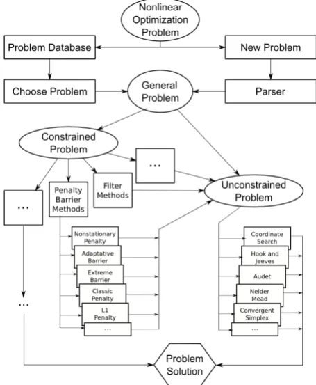
In Fig. 1 are presented all the options available to the user of the developed API.
The developed API, and consequently all applications based on it, allows the user to choose either to use a problem stored in the database or to define a problem to be solved.
If the first option is chosen, then the user can choose among one of the 25 unconstrained problems or one of the 18 constrained problems already available.
If the second option is selected, the user must then choose between constrained and unconstrained problems, define the objective function and the constraints (if any) and define the initial point. Supplied data is then interpreted by an expression parser and a new problem is generated.
After the problem is generated and depending on the type of problem (constrained or unconstrained problem) the user can choose one of the available methods to solve it.
A. Problems with Constraints
If a problem with constraints is chosen, i.e., a problem of the form (2) the user can then choose between: Penalty and Barrier Methods; Filters Method.
These are the methods that are already implemented, but in future other methods will be implemented , such as the Augmented Lagrangian methods.
The objective, when solving a problem with constraints, is to optimize f inΩ, but sometimesf and the constraints are defined outside of Ω. In such cases it is possible to use methods that ”works” outside the feasible region, but it is required, or at least desirable, to find an feasible approximation to the problem solution. However, according to Conn et. al. in [2] and Audet et. al. in [3], f and some constraint functions can not be defined outside ofΩ. Suppose
f or some constraint is just defined in X ∈ Ω, in this case, the constraints that defineX have to be satisfied at all steps in the iterative process for which the objective function (and/or the constraint) is (are) evaluated. Such constraints are notrelaxable. Other constraints only need to be satisfied approximately or asymptotically, these are relaxable.
Thus, one can distinguish Relaxable Constraints and Un-relaxable Constraints.
Definition 1: Constraints functions can be:
• Relaxable Constraints (soft or open) – Constraints that can just be satisfied approximately or asymptotically, being possible to define f and constraints values out-side the region defined by them, conout-sidering a certain tolerance.
• Unrelaxable Constraints(hard or closed) – Constraints that have to be satisfied at all steps in the iterative process, because one or more of the functions involved of the problem are not defined outside of the region defined by them.
1) Penalty and Barrier Methods: Penalty and Barrier Methods have been created to solve problemPdefined in (2), by solving a specially chosen sequence of problems without
IAENG International Journal of Applied Mathematics, 40:4, IJAM_40_4_05
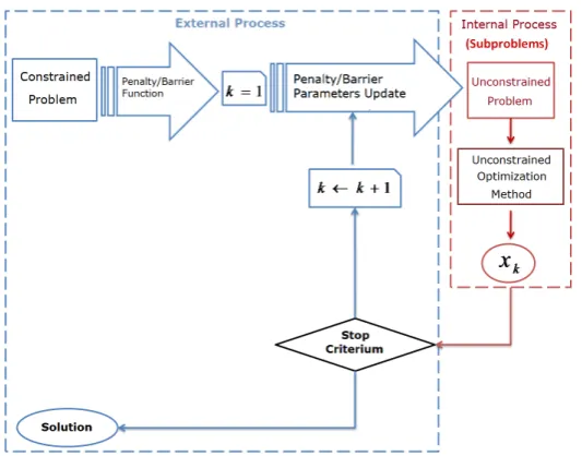
constraints. The original problem is transformed into a sequence of unconstrained problems of the form (1)(External Process) which are solved using methods typically used to solve unconstrained problems (Internal Process). Fig. 2 shows the process diagram block.
In these methods a succession of new objective functions, Φ, for the unconstrained optimization problems, is obtained, which contains information about the initial objective func-tion,f, and the problem constraints, thus the optimality and feasibility are treated together. A succession of unconstrained problems that depend on a positive parameter, rk, which solutionsx∗(rk)converge to the initial problem solutionx∗, is built.
Penalty and Barrier Methods, as presented in Fig. 2, are built by two processes:
• External Process- where a succession of unconstrained problems is created;
• Internal Process - where the unconstrained problems are solved.
The new sequence of problems (of the type (1)) to be solved at each iteration k, that replaces problem P, P(rk) is defined by:
Φ(xk, rk) : min xk∈Rn
f(xk) +rkp(x) (3) where p is a function that penalizes (penalty) or refuses (barrier) points that violates the constraints.
There are several approaches that use this methodology, and it is used in several areas. We can see it being used in Optimizations fields like in context of Linear Optimization, [4]; Particle Swarm Optimization, [5]; Nonlinear Program-ming, [6], [7] and [8] among many others and also in many real applications, for example in [9] and [10].
Of the existing Penalty/Barrier functions we implemented the following: External Barrier Function; Progressive Bar-rier Function; Classical Penalty Function; Static/Dynamic Penalty Function; `1 Penalty Function.
Barrier methods are adequate for solving problems where a feasible approximation to the solution is needed, however the initial point must also be feasible.
The main idea of these methods is reject, in the iterative process, infeasible points and to dissuade the points of any approximation to the feasible region border.
The External Barrier Function, widely used with Direct Search Methods with feasible points, for example by Audet et. al., [11], [12], [13], [14], [15], [3] is defined by:
Φ(x) =
f(x) se x∈Ω
+∞ se x /∈Ω (4)
This function works well with the Direct Search Methods to deal with constraints, because these methods use the objective function value only for comparison in the studied points. So if point falls outside or it approaches the feasible region border Φ = +∞, it is then rejected.
On the other hand, for methods that build models to approximate the objective function this barrier function might not be the most appropriated, since it is a little inflexible because it can eliminate points that can be a good approximation, not to the model but to the objective function.
The need for a feasible initial point caused the develop-ment of a new version of this method, [15], which can also be chosen by the user in the application. In this second version a relaxable constraints violation measurement function is used b : X ⊂ Rn → R+, where a maximum is imposed to the violation value, and points that have a value above this limit are rejected. Authors call Progressive Barrier
to this approach, and MADS-PB (Mesh Adaptive Direct Search - Progressive Barrier) to the method. One advantage of this method is its ability of starting the process with points that violates the relaxable constraints and accepts both testing points and interactions with feasibleviolation to this constraints.
In this method the authors consider the subset X ∈ Ω defined by the relaxable constraints of the problem. If a point is not in X it is rejected, if it is in X then the relaxable constraints (rj(x) ≤ 0, with j = 1, ..., p and where p is the number of relaxable constraints) are treated using the functionbX:Rn →R:
bX(xk) =
m P
i=1
(max (ci(xk),0))2 if x∈X
+∞ if x /∈X
(5)
Note that, consideringxk the iteration to be tested bybX, then bX(xk) = 0 if and only if xk verifies all relaxable constraints of the problem, i.e., ifxk ∈Ω, and ifxk violates any of the relaxable constraints then 0< bX(xk)<+∞ .
Therefore, in each iteration the unconstrained optimiza-tion problem to be solved as the new objective funcoptimiza-tion ΦX(xk) =f(xk) +bX.
This approach is called progressive barrier since it is attributed a maximum value for the violation at each iteration
hkmax, that is progressively updated (iteration by iteration) using a relation of non dominance, used in the Filters Method, between the tested points and withhkmax→0when
k→+∞.
Penalty Methods do not require a feasible initial point to begin the iterative process, however the final approximation to the solution of the problem might be infeasible. Penalty functions penalize the constraints violation, allowing that infeasible points may occur in the iterative process, although penalized, instead of creating a barrier in the border of the feasible region.
In these methods, the feasible region is expanded to Rn,
but a wide penalization, in points that are outside of the original feasible region, is applied to the new objective function of the unconstrained problem.
Classic Penalty Functions include the following type of functions:
ΦX(xk) = f(xk) +rkp(xk) = = f(xk) +rk
m X
i=1
[max{0, ci(xk)}] q
, (6)
withq≥1, and:
• ifq= 1in (6), the functionp(x)is called linear penalty function and the problem to be solved at each iteration, that replaces problem P, is an unconstrained problem
IAENG International Journal of Applied Mathematics, 40:4, IJAM_40_4_05
Figure 2. Penalty and Barrier Methods Implementation Diagram Block
P(rk):
P(rk) : min x∈Rn
f(x) +rk m X
i=1
[max{0, ci(x)}] (7)
wherer={rk}+∞k=1is a succession such thatrk→+∞. • if q= 2in (6), the function p(x) is called a quadratic penalty function and the problem to be solved at each iteration, that replaces problemP, is an unconstrained problemP(rk):
P(rk) : min x∈Rn
f(x) +rk m X
i=1
[max{0, ci(x)}]2 (8) where as aboverk→+∞.
Static Penalty Methods were proposed by Homaifar et al.[16]. In these methods a family of violation levels for each constraint type is used. Each violation level imposes a different penalty. The disadvantage of this method is the number of parameters to be selected early in the iterative process, which rapidly increases with the growth number of constraints and violation levels. A penalty vector is selected for the whole process.
With the penalty vectors α ∈ Rt e β ∈ Rm−t it can
be built, for problem (2), a Penalty Problem (unconstrained problem) for each iterationk, withρ≥1:
min x∈Rn
Φk(x, α, β) (9) with
Φk(xk, α, β) = f(xk) + t P
i=1
αi|ci(xk)| ρ
+
+ m P
i=t+1
βi[max(0, ci(xk)]ρ.
(10)
This Penalty Method can be Exact or Inexact. Ifρ= 1in (10), it is an Exact Penalty Method, ifρ >1it is an Inexact Penalty Method, [17].
The Homaifar’s Static Penalty Method, [16] (1994), has solved a problem similar to (9) with (10), setting the penalty vectors αandβ. This procedure requires the initial selection of a great number of initial parameters (one for
each constraint) and, besides that, it is and Inexact Penalty Method (ρ >1).
As an alternative to the search for the penalty parameters by trial-and-error, there are the Dynamic Penalty Methods [18], that gradually increment the penalties in (9) with Φk defined in (10). They find the global minima ˜xof (9), for each penalty combination and they stop whenx˜is a feasible solution to P, (2).
Many variants of these methods exist. One of them, which is widely known, is theNon-stationary Method that solves a sequence of problems of the same type as (9) withΦkdefined at (10) and ρ >1, updating the penalty parameters at each iteration k, according to the following conditions (C >0 is a constant parameter):
αi(k+ 1) =αi(k) +C.|ci(x)|, i= 1, ..., t (11)
βi(k+1) =βi(k)+C.[max(0, ci(x))], i=t+1, ..., m (12)
`1 Penalty Method was initially proposed by Pietrzykowski [19], and it has been studied and used by many authors, for example Gould et. al. in [20] and Byrd et. al. in [6], furthermore, it has been the base for many penalty methods.
This is a local minimization Exact Penalty Method and it solves at each iterationk the problem:
min xk∈Rn
`(k)1 (xk, µ) (13) with
`(k)1 (xk, µ) = f(xk) +µ t X
i=1
|ci(xk)|+
+ µ
m P
i=t+1
max[ci(xk),0],
(14)
andµ→+∞.
2) Filter Method: To solve a constrained Nonlinear Op-timization Problem (NLP), it must be taken in account that the objective is to minimize the objective function and the constraints violation, that must be zero or tend to zero. This
IAENG International Journal of Applied Mathematics, 40:4, IJAM_40_4_05
involves two concepts:optimality(which has the propose of minimize the objective functionf) and thefeasibility(which is intended to minimize the constraints violations).
In the Penalty/Barrier methods, the optimality and fea-sibility are treated together, however in the Filters Method the concept of bi-objective optimization dominance is used, considering optimality and feasibility separately. In each iteration two phases exist: the first is the feasibility phase and the second is the optimality phase.
The Filters Method was introduced by Fletcher and Leyffer em [21] to globalize SQP (Sequential Quadratic Program-ming) methods and with the motivation to avoid the difficulty in the penalty parameters and/or the Lagrange multipliers estimation. It has been one of the most used techniques in several areas of constrained linear and non-linear optimiza-tion.
A review to the Filters Method was presented by Fletcher et. al. in [22]. In this work they expose the main Filter Methods techniques implemented so far in literature and the main convergence results and also indicate areas where, until then, those methods were used.
This methodology has been applied in several areas of optimization, for example, among others:
1) In Direct Search by Audet and Dennis [23], where Filter Methods are used with Pattern Search Methods, and in Correia et. al. [24], where a new Direct Search Method for Constrained Nonlinear Optimization, that combines the features of a Simplex Method with the Filter Methods techniques. This method, similarly to Audet and Dennis method [23], does not need to calculate or approximate any derivatives, penalty parameters or Lagrange multipliers;
2) In context of non continuous and non differentiable optimization by Fletcher et. al. [25], by Gonzaga et. al. [26] and by Karas et. al. [27];
3) Gould et al. in [28] presents a multidimensional filter and in [29] extends this technique.
4) In SQP by Antunes and Monteiro [30] and by Nie et. al. [31];
5) In Interior Points Methods by Ulbrich et. al. [32]; 6) In a context of Mixed Variable Constrained
Optimiza-tion Problems by Abramson et. al. [33];
7) More recently, one can mention the works of Friedlan-der et al. [34], Luo et al. [35], [36], [37] and Silva et. al. [38].
Filter Methods consider the NLP (2) as a bi-objective program, and it has as main goal the minimization of both the objective function (optimality) and a continuous function
hthat aggregates the problemmconstraint functions values (feasibility).
Priority must be given to hsince it is not reasonable to have as a problem solution a infeasible point, i.e., that does not comply with the constraints.
Therefore, the function hmust be such that:
h(x)≥0 withh(x) = 0 if and only ifxis feasible. We can then define has:
h(x) =kC+(x)k, (15)
where k.k is the norm of a vector and C+(x)is the vector of the t+m values of the constraints in x, i.e, ci(x) for
i= 1,2, ..., t+m:
C+(x) =
ci(x) if ci(x)>0 0 if ci(x)≤0 Considering the norm 1, for example, it is obtained:
h(x) =kC+(x)k1= t+m X
i=1
max (0, ci(x)), Considering the norm2, for example, it is obtained:
h(x) =kC+(x)k2= v u u t
t+m X
i=1
max (0, ci(x)) 2
.
In the API implemented are available, besides these usual measures, more five alternative measures such as presented in [39].
The Filters Method define aforbidden region, memorizing pairs(f(xk), h(xk)), with good performance in the previous iterations, avoiding dominated points (as defined by the current Pareto rule) by the points of this set, in the next iterations.
Definition 2: A point x∈Rn dominates y∈Rn, and is
written as x≺y, iff(x)≤f(y)andh(x)≤h(y).
Definition 3: Afilter,F, is a finite set of points where no pair of points,xandy of the setF, as a relationx≺y, i.e., the filter is made by points such none dominates the other.
A point is accepted by the filter if and only if it is not dominated by other point belonging to the filter and its inclusion eliminates from it all the points that it dominates. We can say that a filter is a dynamic set. A filter works then as a criterion for the iteration acceptance.
Consider the Fig. 3, based on the figure presented by Ribeiro et. al. in [40], that illustrates a filter with four points (represented by a, b, c and d). The Filter points a, b, c
andd define the forbidden region, shaded area. If the point under test is the point represented by y, since it is in the forbidden region it will not be accepted into the filter. But the point represented by z is out of the forbidden region, and therefore it will be accepted and included into the filter. The same applies to the point represented by w, it is not in the forbidden region and therefore it will be accepted and included in the filter, however, in this case, there would still rise to the elimination of points represented by c andd of the filter, since they are in the forbidden region defined by
w, i.e.,canddare dominated byw.
Karas [27], to define a temporary pair for the filter, uses the equality (f(xk), h(xk)) = (f(xk)−αh(xk),(1−α)h(xk)) introducing thereby the envelopeconcept. This modification avoids the acceptance of pairs too close to previous iterations. The concept of envelope is introduced to avoid the ac-cumulation of non-stationary points in the filer, demanding a significant decrease in f or h for each filter input. With this concept it is added a surrounding region to the feasible region, creating a little higher forbidden region and points in this new region are rejected.
Auddet and Dennis, in [11], used for the first time the Filters Method together with the Direct search Methods,
IAENG International Journal of Applied Mathematics, 40:4, IJAM_40_4_05
Figure 3. A Filter with four points (based on Ribeiro et. al. [40]).
namely with Pattern Search Method, showing some conver-gence results. This filter has three main differences to the other filters, according to Fletcher et. al. in [22]:
1) Only needs a simple decrease, similarly to the Pattern Search Methods;
2) The poll center is feasible or is the infeasible iteration with the lower constraint violation;
3) The filter includes a pair (0, fF) that corresponds to the best feasible iteration, i.e., the feasible iteration with the lowest function value found so far in the iterative process.
Let us consider fF the value of the objective function in the best feasible point found until then. Audet filter accepts the point xk if and only if: h(xk) = 0∧f(xk) < fF or
h(xk)< hl∨f(xk)< fl,∀(xl, fl)∈ Fk.
Moreover, it is established a maximum limit to h values of the points accepted in the filter, hmax. Only points xk such that h(xk)< hmax can be included in the filter. This condition avoids the filter to accept points, that even though have an acceptable value forf, are very distant to the feasible region.
These changes were also considered by Correia et. al. in [24] where the Filter Method combined with the Nelder-Mead was implemented and it was compared with Filter Method combined with the Hooke and Jeeves, a Pattern Search Method, this second similarly to what Audet and Dennis did in [23].
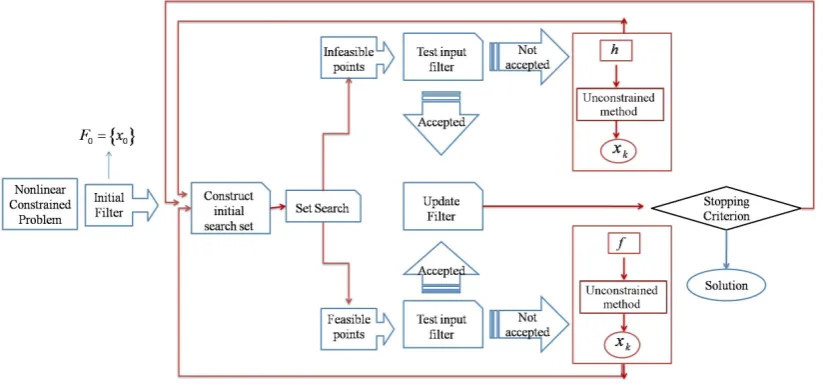
Fig 4 presents the diagram block of the Filter Meth-ods implemented in the API. The implemented algorithm initialise the process constructing the initial Filter which contains the initial point. Then a initial set of search is constructed. In this implementation this set is defined by:
S0 = {x0=v0} ∪ {vi :vi=x0+ei, i= 1, ..., n} where
ei, i = 1, ..., n are the vectors of the usual canonical base in Rn (in the next iterations this set must be Sk =
{xk} ∪ {vi :vi=xk+ei, i= 1, ..., n}, where xk is the current iteration). Then the set search is initialised, beginning with the first point position in the seti= 0.
If the point that is being analysed is a feasible point, its inclusion in the filter is tested:
• If the point is not accepted in the filter:
– An unconstrained optimization method is used to optimize f;
– A new point is obtained;
– Turning to the construction of the set search, from this point.
• If the point is accepted in the filter:
– The filter is updated and this point is considered the new approximation to the solution, i.e., the new iteration;
– If the stop criterion is verified, this approximation is the final approximation to the solution, else go back to the construction of the set search, from this point.
If the point that is being analysed is an infeasible point, its inclusion in the filter is tested:
• If the point is not accepted in the filter:
– An unconstrained optimization method is used to optimize h;
– A new point is obtained;
– Go back to the construction of the set search, from this point.
• If the point is accepted in the filter:
– The filter is updated and this point is considered the new approximation to the solution, i.e., the new iteration;
– If the stop criterion is verified, this approximation is the final approximation to the solution, else go back to the construction of the set search, from this point.
In the end of the process, besides the final solution approximation there are also available the filter points, that are the non dominated points found in the iterative process, so any one of them can be a good approximation solution.
The numerical tests presented in our recent works, Correia et. al. [41], [42], [43], showed that this method is quite effective, in comparison with divers algorithms.
B. Unconstrained Problems
Both for the Penalty/Barrier and the Filters methods it is needed, in the internal process, to solve unconstrained problems with general form like the defined in (1).
Our API and application offers to the user or programmer the following five algorithms to solve such problems:
• A coordinated search algorithm;
• Hooke e Jeeves algorithm;
• A version of Audet et. al. algorithms;
• The Nelder-Mead algorithm;
• A Convergent Simplex algorithm.
These are well known methods found in the specialized literature.
The first three are Pattern Search Methods (described, for example, by Conn et. al. in [2], Chapter 7 - Directional Direct-Search Methods). These methods determine possible optimal points using fixed directions during the iterative process: starting from a iteration xk, the next iteration will be found by searching in a pattern or a grid of points, in the directions d, at a distanceδk (calledstep length).
IAENG International Journal of Applied Mathematics, 40:4, IJAM_40_4_05
Figure 4. Block diagram of the implemented Filters Method
Last two methods are Simplex Methods (described, for example, by Conn et. al. in [2], Chapter 8 -Simplicial direct-search methods). These methods are characterized by starting from an initial simplex and modifying the search directions at the end of each iteration, using movements of refection, expansion and contraction to the inside and the outside, together with the shrunk step towards the best vertex.
III. OPTIONS, VARIABLES ANDPARAMETERS
To solve a problem, regardless of the chosen options, there are parameters that should be defined, while others are set internally, without user intervention.
A. Parameters chosen by the user
For the methods and algorithms to work, besides the problem expression and the initial point, also additional parameters are needed. Some of them are specific to some methods while others are generic. This last set of parameters, which can be changed by the user, are presented in this subsection.
To simplify, in this subsection only the general parameters will be referred, without entering into too much details for those details, although necessary, are too specific to some algorithms.
Generally, it is asked to the user, that he choose or define the following values or parameters, generic to the application:
Input data for the Penalty/Barrier Methods are:
1) Problem to be solved; 2) Initial Point;
3) The penalty/barrier function to be used (1 to 6)
-phi to use;
4) Initial parameters for the penalty/barrier function; 5) Maximum number of external process iterations-kmax; 6) Tolerance for the distance between two iterations -T1; 7) Tolerance between two values of the objective function
in two consecutive iterations -T2; 8) Minimum step length - T3;
9) Method to be used in the internal process - M ET i;
10) Possible change to change the process parameters of the chosen internal process -SouN i;
11) Maximum value of the constraints violation -hmax; 12) Updating factor for the penalty/barrier parameters -γ; Values defined by default in the API are: : kmax = 40,
α= 1,T1 = 0.00001,T2 = 0.00001,T3 = 0.001eγ= 2. In the filters methods input data are, the points above, 1), 2), 5), 6), 7), 9), 10) and the
• The maximum initial value for the constraints violation - hmax;
Parameters defined by default in the API are:kmax= 40e
T1 =T2 = 10−5.
To use the unconstrained methods, previously described in the internal process, it is also needed to define the following parameters:
• Maximum number of internal iterations -kmax; • Initial step length -α:
• Tolerance for the distance between two iterations;
• Tolerance between two values of the objective function in two consecutive iterations;
• Minimum step length;
B. Returning results
The unconstrained methods implemented here, have the following return values:
• Number of objective function evaluations;
• Last values calculated at the Stop Criteria;
• The found solution;
• Value of the objective function at the found solution;
The Filters Methods return the following parameters:
1) Number of internal process iterations; - k; 2) Number of objective function evaluations; 3) Last iteration;
4) Value of the objective function at the last iteration; 5) Best feasible solution (if any);
6) Value of the objective function at the best feasible solution;
7) Iteration at which the best feasible solution was found; 8) Best infeasible solution (if any);
IAENG International Journal of Applied Mathematics, 40:4, IJAM_40_4_05
9) Value of the objective function at the best infeasible solution;
10) Iteration at which the best infeasible solution was found;
11) Value of the constraints violation at the best infeasible solution;
12) Set of non dominated solutions.
Penalty/barrier methods algorithms return the same of the above results, 3), 4), 5), 6), 7), 8), 9), 11) and
• Number of external process iterations;
• Number of Penalty/Barrier function evaluations;
• Value of Penalty/Barrier function at the last iteration;
• Penalty/Barrier function value at the best infeasible solution;
• Iteration were was found the best infeasible solution;
• Constraint violation value at the best infeasible solution;
IV. API IMPLEMENTATION
To obtain platform independence two key technologies must be chosen: the programming technology and the Re-mote Method Invocation technology. The first will define on which platforms the API can be installed, the second will define which technologies will be able to do the remote access.
For the implementation of the API Java Technology was selected, It has official support by Oracle for the most used Operating Systems. However, in this type of applications, not only the portability must be taken in account. Performance is also a key issue.
Several authors have benchmarked Java against other programming languages used in this kind of applications, such as C and FORTRAN [44], and they concluded that it has a good relative performance. In finite element analysis[45] it even has a performance comparable to C. Considering the above presented information, no performance constraints are expected in our API.
The choice of the correct technology for remote access is also very important mater to be considered. The objective is to provide support for remote access for the most used computing platforms and programming languages. The use of Web Services is then a natural choice.
The API can then be accessed in two different ways, one using the standard procedure of installing the .jar
file containing all the developed classes in the developer computer, or remotely accessing the API trough the Local Area Network (LAN) or over the Internet. This last method allows developers and end clients to access always to the latest API version.
A. Using the locally installed API
To use the API from Java applications, using it installed in the local system, the user/programmer needs to save it in the local disc, and include the developed API classor
.jarfile in the classpath. A Class exists for each algorithm and method above mentioned. Fig. 5 shows a sample of Java code where the Pattern Search algorithm is used to minimize an expression.
String expr = ‘‘(x0-2)ˆ2 + (x1+2)ˆ2’’; String initPoint = ‘‘x0=0.0 x1=0.0’’; PatternSearch pattern =
new PatternSearch(expr,initPoit); pattern.run();
double[] result = pattern.getLastResult();
Figure 5. Java code to access the locally installed API - in this example the application executed the Pattern Search algorithm.
The problem expression and the initial point, in this example, are sent to the algorithm using the class constructor. To solve the problem methodrun()is called and results can be obtained by invoking the getLastResult()method. This last methods returns a double array which has the problem dimension.
At any moment setInitialPoint() and
setExpression() methods can be invoked to change the initial point or the problem expression, respectively. Besides these methods, the implemented API also includes methods to set and obtain the parameters and results above mentioned in section III.
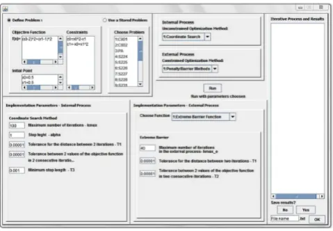
[image:8.595.307.547.398.564.2]An example application developed in Java, that uses the developed API is presented in Fig. 6. This application was developed to demonstrate all the features of the API, and it is to be used as a tool for those that do not want to develop application and only want to use the developed methods.
Figure 6. Example of an application that uses the API installed locally.
B. Remote Access using Web Services
Access to the API as presented in the previous section can only be made if the API is installed on the computer where methods are needed. Besides that, it can only be accessed using Java, since this is the programming technology used in its implementation.
To enable remote access to the implemented methods they were made available using Web Services. By using this technology it is possible to access to them, not only using Java, but also other programming languages used in scientific applications [46] such as FORTRAN, C, C++ and the .NET Framework (C# for example).
Although RMI (Remote Method Invocations) has better performance in Java applications than Web Services[47], they are used in because of its wide compatibility. Also, the
IAENG International Journal of Applied Mathematics, 40:4, IJAM_40_4_05
time spent in communications is much smaller than the time needed to run the optimization methods.
This is mainly due to the fact that Java-RMI uses a binary message format and Web Services use XML(Extensible Markup Language), thus it has a higher protocol overhead.
To access the API, the programmer does not need to install any file on the development computer. It is only needed to have installed the correct development tools. Using the tools provided by the used programming technology, the user must import the WSDL (Web Service Definition Language) file from the URL (Unified Resource Locator)
http://server.address:port/NLOSolver?wsdl, using the correct IP address of the server where the API is installed and correct port number as well. After generating all the locally needed files, the API can then be used.
Sample code showing how to access the remote API using Java is presented in Fig. 7 and Fig. 8 shows sample C# code to access the remote API.
NLOSolverService service =
new NLOSolverService(); NLOSolver nlos =
service.getNLPSolverPort(); String sessionID =
nlos.connect(login,password); String expr = "(x0-2)ˆ2 + (x1+2)ˆ2"; String initPoint = "x0=1 x1=0"; nlos.runPatternSearch
(sessionID, expr, initPoint); List<Double> result =
[image:9.595.342.512.146.279.2]nlos.getPatternSearchLastResult (sessionID);
Figure 7. Java code to access to the remote API using Web Services - in this example the application executed the Pattern Search algorithm.
NLPOolverClient nlps =
new NLOSolverClient(); String sessionID =
los.connect(login, password); String expr = "(x0-2)ˆ2 + (x1+2)ˆ2"; String initPoint = "x0=1 x1=0"; nlos.runPatternSearch
(sessionID, expr, initPoint); double[] result =
nlos.getPatternSearchLastResult (sessionID);
Figure 8. C# code to access the remote API using Web Services - in this example the application executed the Pattern Search algorithm.
Methods available in the remote API include:
connect, to create a new session (needed to deal with multipble access); runMethod, to run a specific method or algorithm, for example:
runAudet, runNelder, runPatternSearch;
getMethodLastResult to fetch the result of a method last run, for example getAudetLastResult,
getPatternSearchLastResult; disconnect to end the session and free all the resources allocated on the server side.
In the example presented in Fig. 7 and Fig. 8 the method connect is used sending two parameters (String) used for
authentication: login and password. Using these credential allows to do access control of the API.
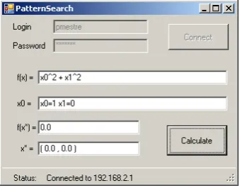
[image:9.595.49.285.291.430.2]An example application developed in C# is presented in Fig. 9. It minimized the expression entered by the user accessing to the API using Web Services. In this particular application the Pattern Search method is used.
Figure 9. Example of an application in C# that acesses to the remote API using Web Services to minimize the function using the Pattern Search Method.
C. Web Application
Besides the Java application above presented, it was also developed a Web-based application, based on the API, accessible using a web browser, to allows users to solve constrained and unconstrained problems, either by choosing one of the problems previously stored in database or by spec-ifying the problem expression and constraints (in constrained problems).
[image:9.595.49.288.479.598.2]This application, which runs on a server and not on the client side, was developed using Java Server Pages (JSP) and it interacts directly with the API. The purpose of this application is to allow users, that do not want to integrated the methods on their applications and simply want to solve a problem. Fig 10 shows the user interface with some of the options available when the user chooses to solve a constrained problem.
Figure 10. Web-based Application
IAENG International Journal of Applied Mathematics, 40:4, IJAM_40_4_05
[image:9.595.325.528.585.771.2]V. CONCLUSION ANDFUTUREWORK
In this paper an API to solve constrained and uncon-strained Nonlinear Optimization Problems was presented. It has been implemented using Java, which makes it compatible with the most used Operating Systems. For those who do not want to install it, or need to access to the API using other programming technology than Java, the developed API supports remote access using Web Services.
Example applications have been presented. Those ap-plications were implemented in Java (accessing the API both locally and remotely) and in C# (accessing the API remotely). However the access to the implemented methods is not restrict to these two programming languages. Any programming language cam be used, as long as it has support for Web Services.
As future work, authors intend to transform the API into a Framework, making it a more powerful for use both in optimization and engineering research.
REFERENCES
[1] J. Matias, A. Correia, P. Mestre, C. Serˆodio, and C. Fraga, “Web-based application programming interface to solve nonlinear optimization problems,” inLecture Notes in Engineering and Computer Science - World Congress on Engineering 2010, vol. 3. London, UK: IAENG, (2010), pp. 1961–1966, ”Certificate of Merit for The 2010 International Conference of Applied and Engineering Mathematics” WCE - ICAEM’10.
[2] A. R. Conn, K. Scheinberg, and L. N. Vicente, Introduction to Derivative-Free Optimization. Philadelphia, USA: MPS-SIAM Series on Optimization, SIAM, (2009).
[3] C. Audet, J. E. D. Jr., and S. L. Digabel, “Globalization strategies for mesh adaptative direct search,” Les Cahiers du GERAD, ´Ecole Polytechnique de Montr´eal, Tech. Rep. G-2008-74, (2008). [4] P. Moengin, “Polynomial penalty method for solving linear
pro-gramming problems,” IAENG International Journal of Applied Mathematics, vol. 40(3), p. Online publication: IJAM 40 3 06, (2010).
[5] M. Pant, R. Thangaraj, and V. P. Singh, “Particle swarm optimization with crossover operator and its engineering applications,” IAENG International Journal of Computer Science, vol. 36(2), p. Online publication: IJCS 36 2 02, (2009).
[6] R. H. Byrd, J. Nocedal, and R. A. Waltz, “Steering exact penalty methods for nonlinear programming,” Optimization Methods & Software, vol. 23, no. 2, pp. 197–213, (2008).
[7] L. Chen and D. Goldfarb, “Interior-point l(2)-penalty methods for nonlinear programming with strong global convergence properties,”
Mathematical Programming, vol. 108, no. 1, pp. 1–36, (2006). [8] S. Leyffer, G. Calva, and J. Nocedal, “Interior methods for
mathematical programs with complementarity constraints,” SIAM Journal on Optimization, vol. 17, no. 1, pp. 52–77, (2006). [9] P. Nanakorn and K. Meesomklin, “An adaptive penalty function in
genetic algorithms for structural design optimization,”Computers & Structures, vol. 79, no. 29-30, pp. 2527 – 2539, (2001).
[10] T. Ibaraki, S. Imahori, K. Nonobe, K. Sobue, T. Uno, and M. Yagiura, “An iterated local search algorithm for the vehicle routing problem with convex time penalty functions,”Discrete Applied Mathematics, vol. 156, no. 11, pp. 2050 – 2069, (2008).
[11] C. Audet and J. E. D. Jr., “Analysis of generalized pattern searches,”
SIAM Journal on Optimization, vol. 13, no. 3, pp. 889–903, (2002). [12] C. Audet, “Convergence results for pattern search algorithms are tight,”
Optimization and Engineering, vol. 2, no. 5, pp. 101–122, (2004). [13] C. Audet, V. B´echard, and S. L. Digabel, “Nonsmooth optimization
through mesh adaptive direct search and variable neighborhood search,”J. Global Opt., no. 41, pp. 299–318, (2008).
[14] C. Audet and J. E. D. Jr., “Mesh adaptive direct search algorithms for constrained optimization,”SIAM Journal on Optimization, no. 17, pp. 188–217, (2006).
[15] ——, “A mads algorithm with a progressive barrier for derivative-free nonlinear programming,” Les Cahiers du GERAD, Ecole´ Polytechnique de Montr´eal, Tech. Rep. G-2007-37, (2007). [16] A. Homaifar, S. H. V. Lai, and X. Qi, “Constrained optimization via
generic algorithms,”Simulation, vol. 62, no. 4, pp. 242–254, (1994).
[17] D. P. Bertsekas,Nonlinear Programming. Belmont, Massachusetts: Athena Scientific, (1999).
[18] F. Y. Wang and D. Liu, Advances in Computational Intelligence: Theory And Applications (Series in Intelligent Control and Intelligent Automation). River Edge, NJ, USA: World Scientific Publishing Co., Inc., (2006).
[19] T. Pietrzykowski, “An exact potential method for constrained maxima,”
SIAM Journal on Numerical Analysis, vol. 6(2), pp. 299–304, (1969). [20] N. I. M. Gould, D. Orban, and P. L. Toint, “An interior-pointl1-penalty
method for nonlinear optimization,” Rutherford Appleton Laboratory Chilton, Tech. Rep., (2003).
[21] R. Fletcher, S. Leyffer, and P. L. Toint, “On the global convergence of an slp-filter algorithm,” Dundee University, Dept. of Mathematics, Tech. Rep. NA/183, (1998).
[22] ——, “A brief history of filter method,” Argonne National Laboratory, Mathematics and Computer Science Division, Tech. Rep. ANL/MCS-P1372-0906, (2006).
[23] C. Audet and J. Dennis, “A pattern search filter method for nonlinear programming without derivatives,” SIAM Journal on Optimization, vol. 5, no. 14, pp. 980–1010, (2004).
[24] A. Correia, J. Matias, P. Mestre, and C. Serˆodio, “Derivative-free optimization and filter methods to solve nonlinear constrained problems,”International Journal of Computer Mathematics, vol. 86, no. 10, pp. 1841–1851, (2009).
[25] R. Fletcher and S. Leyffer, “A bundle filter method for nonsmooth nonlinear optimization,” Dundee University, Dept. of Mathematics, Tech. Rep. NA/195, (1999).
[26] C. Gonzaga, E. Karas, and M. Vanti, “A globally convergent filter method for nonlinear programming,”SIAM Journal on Optimization, vol. 14, no. 3, pp. 646–669, (2003).
[27] E. W. Karas, A. A. Ribeiro, C. Sagastiz´abal, and M. Solodov, “A bundle-filter method for nonsmooth convex constrained optimization,”
Mathematical Programming, vol. 1, no. 116, pp. 297–320, (2006). [28] N. Gould, S. Leyffer, and P. Toint, “A multidimensional filter algorithm
for nonlinear equations and nonlinear least-squares,”SIAM Journal on Optimization, vol. 15, no. 1, pp. 17–38, (2005).
[29] N. Gould, C. Sainvitu, and P. Toint, “A filter-trust-region method for unconstrained optimization,”SIAM Journal on Optimization, vol. 16, no. 2, pp. 341–357, (2006).
[30] A. Antunes and M. Monteiro, “A filter algorithm and other nlp solvers: Performance comparative analysis,”Lecture Notes in Economics and Mathematical Systems - Recent Advances in Optimization, vol. 563, pp. 425–434, (2006).
[31] P. Nie, “Sequential penalty quadratic programming filter methods for nonlinear programming,”Nonlinear Analysis-Real World Applications, vol. 8, no. 1, pp. 118–129, (2007).
[32] M. Ulbrich, S. Ulbrich, and L. Vicente, “A globally convergent primal-dual interior-point filter method for nonlinear programming,”
Mathematical Programming, Ser. A, vol. 2, no. 100, pp. 379–410, (2004).
[33] M. Abramson, C. Audet, and J. D. Jr., “Filter pattern search algorithms for mixed variable constrained optimization problems,”Pacific Journal of Optimization, no. 3, pp. 477–500, (2004).
[34] M. Friedlander, N. Gould, S. Leyffer, and T. Munson, “A filter active-set trust-region method,” ANL/MCS-P1456-0907, Tech. Rep., (2007). [35] H. Luo, “Studies on the augmented lagrangian methods and convexification methods for constrained global optimization,” Ph.D. dissertation, Department of Mathematics, Shanghai University, Shang-hai, (2007).
[36] H. Luo, X. Sun, and D. Li, “On the convergence of augmented lagrangian methods for constrained global optimization,” SIAM Journal on Optimization, no. 18, pp. 1209–1230, (2007).
[37] H. Luo, X. Sun, and H. Wu, “Convergence properties of augmented Lagrangian methods for constrained global optimization,” Optimiza-tion Methods & Software, vol. 23, no. 5, pp. 763–778, (2008). [38] R. Silva, M. Ulbrich, S. Ulbrich, and L. Vicente, “A globally
convergent primal-dual interior-point filter method for nonlinear programming: new filter optimality measures and computational results,” Dept. Mathematics, Univ. Coimbra, Tech. Rep. Preprint 08-49, (2008).
[39] A. Correia, J. Matias, P. Mestre, and C. Serˆodio, “Direct search filter methods,” inBook of Abstracts of the 24nd European Conference on Operational Research, Lisbon, Portugal, (2010).
[40] A. Ribeiro, E. Karas, and C. Gonzaga, “Global convergence of filter methods for nonlinear programming,”SIAM J. on Optimization, vol. 19, no. 3, pp. 1231–1249, 2008.
[41] J. Matias, A. Correia, P. Mestre, and C. Serˆodio, “Derivative-free nonlinear optimization filter simplex,” in Book of Abstracts of the
IAENG International Journal of Applied Mathematics, 40:4, IJAM_40_4_05
XV International Conference on Mathematics, Informatics and Related Fields, Pol´onia, (2009), p. 47.
[42] A. Correia, J. Matias, P. Mestre, and C. Serˆodio, “Penalty versus filter methods,” inBook of Abstracts of the 23nd European Conference on Operational Research, Bonn, Alemanha, (2009), p. 189.
[43] ——, “Derivative-free nonlinear optimization filter simplex,” Interna-tional Journal of Applied Mathematics and Computer Science (AMCS), vol. 20, no. 4, (In Press, 2010).
[44] J. M. Bull, L. A. Smith, C. Ball, L. Pottage, and R. Freeman, “Benchmarking Java against C and Fortran for scientific applications,”
Concurrency and Computation: Practice and Experience, vol. 15, no. 3-5, pp. 417–430, March-April 2003.
[45] G. P. Nikishkov, Y. G. Nikishkov, and V. V. Savchenko, “Comparison of C and Java performance in finite element computations,”Computers & Structures, vol. 81, no. 24-25, pp. 2401–2408, September 2003. [46] R. A. van Engelen, “Pushing the SOAP Envelope WithWeb Services
for Scientific Computing,” in Proceedings of the International Conference on Web Services (ICWS), 2003, pp. 346–352.
[47] M. B. Juric, I. Rozman, B. Brumen, M. Colnaric, and M. Hericko, “Comparison of performance of Web services, WS-Security, RMI, and RMI-SSL,”Journal of Systems and Software, vol. 79, no. 5, pp. 689– 700, May 2006, quality Software.
![Figure 3.A Filter with four points (based on Ribeiro et. al. [40]).](https://thumb-us.123doks.com/thumbv2/123dok_us/387617.536282/6.595.66.268.55.220/figure-filter-points-based-ribeiro-et-al.webp)