AN ENERGETIC VARIATIONAL APPROACH TO MATHEMATICAL MODELING OF CHARGED FLUIDS: CHARGE PHASES, SIMULATION AND WELL POSEDNESS
A Thesis in Mathematics
by
Rolf Josef Ryham
c
2006 Rolf Josef Ryham
Submitted in Partial Fulfillment of the Requirements
for the Degree of
Doctor of Philosophy
Chun Liu
Professor of Mathematics
Thesis Advisor, Chair of Committee
Ludmil Zikatanov
Professor of Mathematics
Thesis Co-Advisor, Co-chair of Committee
Qiang Du
Professor of Mathematics Internal Committee Member
Yousry Azmy
Professor of Nuclear Engineering External Committee Member
Fanghua Lin
Silver Professor of Mathematics, Courant Institute, NYU Special Member
John Roe
Professor of Mathematics Department Chair
In thesis we propose a mathematical model of electrolyte fluid and interface sys-tems. The model is based on a coupling between the Navier-Stokes equations of an incompressible fluid, the Nernst-Plank-Poisson equations of a diffuse, binary elec-trolyte, and the phase field Allen-Cahn equation. The coupling is derived in the energetic variational framework and guarantees the consistent exchange of the ki-netic energy of the fluid, entropic and electric energy of the charge carriers and the surface area of the interface. Using the phase field as a topological labeling of the interface, we introduce a “short range” barrier potential which selectively blocks charge migration across the interface. The model is able to capture the dynamics of both charge induced flow and selection by the interface. This is demonstrated by simulation of the coalesence of two charge selective vesicles by charge induced motion.
We also develope the existence theory for global classical solutions of the NPP equations with smooth data in space dimensiond≤3,global weak solutions to the NPP equations coupled with the NS equations ford≤3 and global weak solutions for small initial data with the additional phase field Allen Cahn equation in space dimension d ≤ 2. The NPP equations are a system of second order, divergence form, semilinear, nonlocal parabolic equations. We elucidate many of the special features of the NPP equations which are nonstandard in complex fluid systems.
List of Figures vi
Acknowledgments vii
Chapter 1 Introduction 1
1.1 Permselective Membranes . . . 4
1.2 Energetic Formulation . . . 6
Chapter 2 The Energetic Variational Approach 8 2.1 Interfacial Energies . . . 9
2.2 Least Action Principle and Variational Derivatives . . . 12
2.3 The Nernst-Plank-Poisson Equations . . . 16
Chapter 3 Charge Phases 19 3.1 Introduction . . . 19
3.2 Phase field barrier functional . . . 21
3.3 A model of electrolyte droplets . . . 24
3.4 Free energy variation . . . 25
3.5 Verification for transport case . . . 27
3.6 Simulation . . . 31
3.7 Conclusion . . . 35
Chapter 4 Classical and Weak Solutions 37 4.1 Preliminaries . . . 37
4.2 Classical Solutions to PNP Equations . . . 39
4.3 PNP and NS Coupling . . . 46
4.4 PNP, NS, Allen-Cahn Coupling . . . 53
5.2 Stationary Solutions . . . 57 5.3 Plug Flow . . . 68
Bibliography 70
3.1 Two phase fluid model of electrolyte droplet. . . 20
3.2 Finite element simulation of droplet coalescence . . . 22
3.3 Evolution of phase field energySη(φ) for a variety of applied fieldsE. . . 33
3.4 Evolution of phase field for two oppositely charged droplets. . . 33
3.5 Mass conservation with respect toU(t) . . . 35
3.6 Mass conservation in domain and change in surface energy . . . 35
5.1 Numerical demonstration of upper bound of solution maximum. . . 67
I would like to express my deepest gratitude to my advisors; Professors Chun Liu and Ludmil Zikatanov. I am forever indebted to them for their guidance and will always treasure their friendship.
Portions of this thesis were completed while the I was visiting the Institute for Mathematics and its Applications in Minneapolis and at the Lawrence Livermore National Lab. I am grateful for their support and hospitality. I would also like to acknowledge the partial support of the National Science Foundation through grants and the VIGRE graduate fellowship.
Much of thesis was also motivated and assisted by discussions with Professors Qiang Du, Douglas Arnold, Martin Bazant, Fang-Hua Lin, Qi Wang, and Zhi-Qiang Wang.
This thesis is dedicated to my father Rolf, whose reflection I see in myself more and more as I grow older, to my mother Christine, whose constant support, sympathy and compassion are felt even in those around me, to my brother Patrik, whom I dearly miss, to my bff STM, to ACD, who taught me to be brave, and finally, to Aur´elie, whose grace and tenderness remind me why life is beautiful.
Introduction
A well established model for charged fluids is given by the transport and Lorentz force coupling between the Navier-Stokes equations of an incompressible fluid and the transported Poisson-Nernst-Plank (PNP) equations of a binary, diffuse charge system [42, 46, 44, 45]. The equations are
ρ(ut+u· ∇u) +∇π=ν∆u+ (n−p)∇V, (1.1)
∇ ·u= 0, (1.2)
nt+u· ∇n=∇ ·(Dn∇n−µnn∇V), (1.3)
pt+u· ∇p=∇ ·(Dp∇p+µpp∇V), (1.4)
∇ ·(ǫ∇V) =n−p. (1.5)
u is the fluid velocity, π is the pressure, ρ is the fluid density and ν the fluid viscocity. n and p are the density of binary diffuse negative and positive charges respectively;Dn, Dpandµn, µpare their respective diffusivity and mobility tensors. ǫis the dielectric constant of the fluid. In this work we consider the caseρ=Dn =
Dp =µn=µp = 1. ǫ is taken to be a constant1. In chapter 5, we consider the case stationary solutions of (1.1)-(1.5) when ǫ→0.
Several classical and contemporary experimental phenomena can be theoreti-cally and numeritheoreti-cally recovered from this system of equations. They include the
1ǫ2=ǫ
0ǫrkT /(C∞L)e2, whereǫ0is the permittivity of vacuum,ǫris the relative permittivity,
kT is thermal energy,C∞ is the characteristic charge density,eis the elementary charge andL
is the characteristic length scale. Typically,ǫranges from 10−3 to 10−6 for realistic systems on
motion of charge selective, conducting or polarizable particles and the induced mo-tion of fluids. These phenomena arise as a result of polarized concentramo-tion layers at the boundary interface between the charged fluid and inclusions [52, 42, 44]. It is in this charged induced motion that electro kinetics becomes a key tool in micro fluidic devices with applications to fluid pumping and particle selection.
Traditionaly, (1.1)-(1.5) are posed in a fixed domain. In this work we couple equations (1.1)-(1.5) with the Allen-Cahn equation as a diffuse formulation of a moving boundary interface. The boundary interface partitions the domain into a region where the dynamics of the charge system are seperated from the other region. As is the case with many interface boundary systems, the modeling of boundary kinetics becomes difficult due to the mixing of coordinate systems. This problem is especially apparent when the interface is free to move or the functions defined over the regions separated by the interface are coupled through boundary condition. In electrolyte systems especially, many experimental observations have yet to be recovered by correct boundary kinetic formulations. A major focus of studies in electrolyte research attempts to understand the interface boundary condition coupling of the diffuse charged bodies and electrostatic potential. From a theoretical standpoint, the interface also represents a difficulty in the existence and regularity theory. The authors demonstrated in [48] that without the presence of an interface, the system (1.1)-(1.5) is totally dissipative. The presence of a boundary, however, introduces terms which are not amenable to producing apriori estimates. The reader should understand that this irrespective of the zero Debye length limit and is a misfeature of the PDE.
equation. Chapter 5 is devoted to stationary solutions of (1.1)-(1.5) in the limit
ǫ→0.
The question of existence of classical solutions to the PNP equations (and weak solutions to the PNP and NS coupling) is nontrivial. The PNP equations are a second order, divergence form, semilinear, nonlocal system. The nonlocal convective term in the equations for n and p ∇V is self induced by the Poisson equation (1.5). The potentialV is repulsive in the sense that the sign dependence on V in (1.4) and (1.5) is opposite of the sign dependence on n in (1.5) and p in (1.5). Thus the equation dynamic results in a dissipation of the potential energy due to V. If the sign dependence were switched (as is the case for the equations of chemotaxis, see [22]), i.e. the self induced potential is attractive, then such a system is degenerate and exhibits finite-time blow-up solutions. This indicates that the existence of global solutions has a nontrivial dependence on the equation structure.
1.1
Permselective Membranes
Equations (1.1)-(1.5) are in the majority studied in the context of permselective membranes2. A permselective membrane is the boundary interface between an electrolyte (liquid) solution and a solid or liquid region which is selectively per-meable. Selectively permeable means that the junction permits currents of one (or none) of the charge species. Studies of permselective membranes account for the relationship between the current of this particular species and the difference in voltage (potentential) between the boundary interface and the bulk of the elec-trolyte.
There is a region of concentration polarization near the boundary interface. A concentration polarization refers to the boundary layer at the boundary interface where the charge densities are, in general, different3. The structure of the bound-ary layer has a complicated dependence on the potential difference and the current of the charge species at the junction. The complexity of this boundary layer has historically lead to numerous formulations of boundary conditions and approxi-mations of the governing equations (1.1)-(1.5). It is worth pointing out that no boundary conditions have yet been formulated which satisfactorily account for the experimentally observed relationships between current and voltage. Three inter-esting, contemporary formulations of the boundary layer structure question the validity of the governing equations in the region of concentration polarization.
One formulation focuses on the ion transport in membranes where the permse-lective interface is a membrane with open channels. Potassium channels (a typical integral membrane protien) have an overall length of 45 ˚A and a 10 ˚A diame-ter cavity. The differing dielectric properties of the surrounding protien and lipid membrane (solid) and the open channels (aqueous) at a scale comparable to the length scale of the governing equations make it difficult to (formally) calculate the induced surface charge and potential within the channel, [24]. If the radius of hydrogen is 0.5 ˚A, then such a channel would allow for the presence of atmost
π(20)2 ≈ 1200 particles. Describing this system by a continuum distribution is questionable. Nevertheless such a study is of great importance considering that
2Similar equations have been extensively studied in semiconductor device, electrochemical
film, and fuel cell models.
all extracellular regulatory mechanism occur through a membrane ion transport. A notable study of ion transport in open channels is [51, 40]. Beginning from the equations of motion for individual ions the authors have derived a modified version of the diffuse equations (1.4)-(1.5), to include forces induced by self induced sur-face charges. They have called this the Coniditional Poisson-Nernst-Plank (CPNP) system. An older study by [18, 19] derives the induced surface charge when an arbitrary charge distribution is given.
Two other areas of study have postulated the existence of additional dynam-ics at the electrolyte junction. The work by [47] has given convincing numerical evidence that electro-osmotic convection at the electrolyte junction induces a pe-riodic vorticity in the flow along the interface. They claim that the convection due to a fluid instability is the source of overlimiting conductance, rather than the traditional thought that it is simply due to electroconvection. In discussion, though, Rubinstein has conceded that this instability has not been experimentally observed. A more recent attempt by [20] has considered modifying the free energy of the charge system to include steric effects, namely that the charge density at the junction is limited by the finite radius of the individual ions. Following [21], they introduce the additional entropic contribution to account for the order a3 solvent displacement by ions of radiusa.This approach is similar to ours, as we introduce in Chapter 3 a free energy that penalizes for the presence of ions in regions exterior to the electrolyte (see equation (3.14).)
the boundary and that the potential φ diverges to ±∞ uniformly away from the interface. The assignment of fixed boundary conditions for either charge species then becomes an unrealistic assumption because the value of either charge species at the interface can be parametrized by ǫ and the total net charge! One might argue, though, that an electrolyte of nonzero net charge does not exist, along with said instability. This is in a sense true, to the degree of what one means by zero net charge. If a current is present at the electrolyte junction, then a change in the net charge, although slight, might be significant with respect to ǫ to induce the above mentioned instability. This being said, we claim that any asymptotic expansion of
n, p and φ with respect to ǫ is unjustified without first explicitly guaranteeing or specifiying that the total net charge is “small” compared to ǫ. We plan to extend the results of Chapter 6 to more general boundary conditions of the potential φ
and to include the nonzero current/boundary flux case.
1.2
Energetic Formulation
The charge PNP equations stems from a well defined free energy consisting of the electric and entropic energy. Other energetic contributions, such as those leading to induced surface charges [40], steric effects [20] and other forces can similarly be accounted for by modifications of the free energy. Also, the force induced by the charge system on the fluid, (in our case (n−p)∇V in equation (1.1)) is similarly derived from this free energy (see Chapter 2, section 2.2). A major contribution of this work is formulation the hydrodynamic system (1.1)-(1.5) and the PNP equations themselves in terms of energetic principles at the continuum level. To clarify, the equations of motion
¨
x−γ−1x˙ =∇F(x), x∈
RN, N ≫1
particle positions leads to the the Liouville (conservation of mass) equation. This is our point of departure, namely in correctly formulating the force ∇F in terms of the continuum distribution of x.
There are several consequences of such a formulation. The first and most im-portant consequence is the differential inequality describing the exchange between kinetic and free energy of the charge system (see equation (2.14) with variants (3.30) and (4.31)). We refer to this differential inequality as the canonical energy law. In the mathematical existence theory this DI is the source of apriori bounds which are so critical in the construction of approximate solutions. This object, which is natural to study from the mathematical standpoint, also captures the physical force balance of the system; it states that the exchange of kinetic and free energy is lost to diffusion and viscous damping. In equations (1.4)-(1.5) the fluid imparts a force on the charge system through transport while in equation (1.1) the charge system imparts the Lorentz force on the fluid. From the modeling point of view, any formulation which does not reflect this force balance relationship in an energy law cannot be faithful to the dynamic.
This admonishen holds for numerical approximations as well. In order for the numerical approximation to be faithful to the force balance dynamic it must also satisfy a discrete form of the canonical energy law. For example, in existence proofs found in Sections 4.2 and 4.3, it quickly becomes apparent solutions and solution approximations of the PNP equations must be strictly positive for the canonical energy law to hold. To address this need, we have chosen a numerical discretization4 of equations (1.4) and(1.5) which preserves the positivity of the diffusion-convection operator under the assumption that the domain triangulation (tetrahedralization in three dimensions) is Delaunay. Furthermore, when the prob-lem being considered has solutions limiting to a simgular probprob-lem, e.g. ǫ → 0 in (1.5), then the only physically relevent approximations captured by the numerical scheme will be those with energies bounded irrespective ofǫ.
The Energetic Variational
Approach
The energetic variational approach to complex fluid problems consists of postu-lating energies that approximate the energy of internal variables of the complex fluid, and defining energetically consistent evolution equations. By consistent, we mean that the net exchange of the internal variables’ energies and kinetic energy, ignoring viscous losses, is zero. A general framework for producing such evolu-tion equaevolu-tions relies on two variaevolu-tion principles; the least acevolu-tion principle and the principle of steepest descent. The least action principles stipulates that the fluid minimizes the loss of kinetic energy to the energy of internal variables. The law of steepest descent stipulates that the internal variable chooses an evolution path which minimizes the internal energy most quickly. The choice of this path is of the gradient descent with respect to the internal energy where the gradient is de-fined by the admissable perturbations of the internal variable. The consistency of the system is a generic consequence of the coupling through transport and force balance. In some notable cases, the consistency of the complex fluid system is key to developing an existence theory and developing numerical strategies which guarantee stability. This is unfortunately not the case for the system considered in this work.
Two of these notable complex fluid systems are liquid crystals, viscoelastic fluids and fluid structure systems.
Nernst-Plank-Poisson (NPP) equations with the presence of an interface for the most simple set-ting; the evolution of charged fluids where the charge system is simply restricted to the interior of an interace. This system requires us to consider several energetic constructs. The first will be the implicit description of the interface by the phase-field labeling function. We will introduce the necassary variational formalism and derivation of the force balance equations via the least action principle. With these tools we derive the NPP equations and Lorentz force coupling with the fluid. In chapter 3, we introduce an additional interface/phase field dependent potential to charge system.
As elluded to before, the energetic vartional framework guarantees the consis-tency between the kinetic and internal energy transfer. Additional estimates must be made for the charge densities to gaurantee the existence of solutions with the fluid coupling. The canonical internal energy of diffuse systems implies no addi-tional regularity of solutions other than integrability. Below we give a thorough outline of the implicit description by the phase field internal variable, the deriva-tion of orce balance equaderiva-tions by the least acderiva-tion principle and introduce several notions and aspects of variational derivatives.
2.1
Interfacial Energies
In general, the interface between regions Γ(t) evolves according to its interfacial energy dissipation. The interfacial energy, denotedS,is exchanged with the kinetic energy of the surrounding fluid and the energy of other internal variables, e.g. the electric and entropic energy of the charge system. The exchange of energy with the charge system is realized by restriction of the charged bodies to regions specified by the interface. The exchange with kinetic energy is realized through interfacial forces as governed by S. In return, the interface, viewed as a two dimensional region of the fluid, is transported by the fluid flow field.
are described by Eulerian variables. Traditionaly, there are several well-established methods of analytically and computationally modeling surfaces. Most notably, these include direct methods, the front tracking [1, 2], volume of fluid (VOF) [3], and level set methods [4], [14].
The most straight forward way of handling a moving surface is the direct method. One employs a discretization with grid points on the surface itself, using finite differences, finite-elements, and boundary-integral techniques. Although con-ceptually convenient, this method inherits the trappings of a moving mesh scheme. Large deformations in the surface may lead to mesh entanglement, and keeping track of the mesh requires a great deal of algorithmic complexity. Most impor-tantly though, it is difficult to couple the surface motion with the field equation of a body force, making interface motion through a fluid difficult to model.
Alternatively, one may fix a discretization of the domain, and represent the surface motion as a vector field distributed along a thin band within which the surface resides. Methods of this type include the level set, VOF, and front track-ing methods. The advantage here is that the surface motion, although distributed over a small region, is a bulk quantity and couples easily with other fields. Fur-ther, there is no algorithmic overhead in keeping track of the quality of the domain discretization. The above mentioned schemes, however, do not treat the discretiza-tion uniformly on the whole domain. Front tracking requires the soludiscretiza-tion of an auxiliary Riemann problem to extrapolate the difference scheme at the interface. In the other models, the indicator function must be renormalized at each time step, introducing artificial dampening to the surface motion.
The phase field is a topological labeling of the interior and exterior of the interface in the domain Ω⊂Rdby the values 1 and -1. The transition region, where
φ deviates from these two values, is where the associated energy density ofSη and consequently interfacial force are supported. η is the order parameter describing the characteristic thickness of the interfactial region. The interface Γ(t) is now loosly associated with this region, motivating another phase field nomenclature, the diffuse interface. In the limit η→0, the phase field approaches the something like the characterstic function of the interior and exterior of Γ(t) while the diffuse interface forces heuristically approach those of the the original sharp interface dynamic. The sharp interface limit of phase field dynamics is popular topic of research and the convergence of energy and force terms for all but the most simple energies remain largely unknown. The reader intersted in these results may further investigate the references given herein.
The interfacial energySη(φ) of the phase fieldφdepends on the type of interface being considered. For example, if the interface Γ(t) = {φ= 0}models the junction between two immisable fluids, then the energy
Sη(φ) =
Z
Ω 1 2η|∇φ|
2+ 1
ηW(φ)dx, W(φ) =
1 4(φ
2
−1)2 (2.1)
approximates the surface area of Γ(t) in the limit η → 0. Loosly speaking, if Sη
Other forms of the functionalSη approximate more general interfacial energies;
In the case of membrane vesicles, where Γ(t) models a lipid membrane for example
Z
Ω
η
2
∆φ− 1 η2W
′(φ)
2 dx≈
Z
Γ(t)
H2dS (2.2)
is a good approximation of the mean curvature energy or in the case of the topo-logical index of the vesicle,
Z
Ω
η∆φ− 1 ηW
′(φ)
W′(φ)dx≈ Z
Γ(t)
K dS (2.3)
approximates the Euler number of {φ = 0}. K = k1k2 and H = (k1 +k2)/2 are of course the Gaussian and mean curvature of Γ(t) respectively. Unlike, (2.1), not a great deal is known about the asymptotic behaviour, existence of minimizers or existence of time dependent solutions given by (2.2) (see [43, 39] for two recent developements). The minimization of (2.2) is related to the Willmore problem from differential geometry, [57]. This author and collaborators have proposed (2.2) and (2.3), and the resulting hydrodynamic equations in the study of vesicle membranes. We have demonstrated the convergence of these functionals to their geometric analogues under the somewhat restrictive ansatz that φ satisfy an optimal profile condition [26, 27, 31]. However, our collaborators have simulated the minimization and hydrodynamic coulping of (2.2) and (2.3) which are encouraging results as to the viability of phase field modeling of vesicle membranes, [25, 26, 29, 30].
2.2
Least Action Principle and Variational
Derivatives
variation with respect to the predomain.
Assume that ψ : Ω→Ris a function, the internal variable, and
L(ψ) =
Z
Ω
Q(ψ,∇ψ)dx (2.4)
is a functional, the internal energy. A variational derivative of L, if it exists, is defined as the limit
lim
s→0 1
s(L(ψ s)
−L(ψ0)) (2.5)
whereψsis a one parameter family of functions chosen with respect to a particular
type of test function, or perturbation.
The usual Frechet derivative, denoted simply by Lψ or L′ (in case it is clear thatLdepends only on one function, the prime (·)′ notation is used), is defined by
hLψ, ui=
Z
Ω
(Qψ− ∇ ·Q∇ψ)u dx, ∀u∈Cc∞(Ω).
The perturbation in this case is a solution to the equation ∂sψs+u = 0, ψ0 =ψ. The space of test functions for the Frechet derivative are maps from Ω intoRwhich are added to the functional argument.
In contrast, in the variation of the domain, the variation is chosen from maps from Ω to itself. The test space is the tangent space of diffeomorphisms of Ω The variation of the domain derivative, denoted Lψ
∗, is given by hLψ∗,ui=−
Z
Ω
(Qψ − ∇ ·Q∇ψ)∇ψ·udx, ∀u∈(Cc∞(Ω))2. (2.6)
In this case, the pertubation occurs within the argument of ψ itself, so that ψs
solves the transport equation ∂sψs+u· ∇ψs = 0, ψ0 = ψ. The variation of the
domain describes the pertubation of those internal variables which are moving with the fluid, e.g. a material labelings or densities of very small, dilute particles.
If ψ is the density of particles indexed by points in the conitunuum W with positions in Ω, then a third variation is chosen from the tangent space of maps into Ω from the predomain W.The deviation of the the variable ψ is motivated as follows. Suppose that ψs is defined as a constant multiple of the Jacobian, Js of
fieldv: Ω→R3 by v(xs) =∂
sxs. We may compute the deviation ofψs as follows;
for any y∈C∞ 0 (Ω),
Z
Ω
∂sψ(X)y(X)dX= d
ds Z
Ω
det(Js((xs)−1(X)))ψ0((xs)−1(X))y(X)dX
= d
ds Z
W
ψ0(w)y(xs(w))dw =
Z
W
ψ0(w)∇y(xs(w))·∂sxs(w)dw
=
Z
Ω
det(Js((xs)−1(X)))ψ0((xs)−1(X))∇y(X)·v(X)dX
=−
Z
Ω∇ ·
(ψs(X)v(X))y(X)dX.
As the above identity holds for all y, we have that the class of all admissable perturbations to functions of the formψs(xs) = det(Js)ψ
0.is given by solutions to the equation∂sψs+∇·(ψsv) = 0.The derivative with respect to such perturbations, L∗ψ, is defined where ψs is a solution to the convection equation, hence
hL∗ψ,ui=−
Z
Ω
ψ∇(Qψ− ∇ ·Q∇ψ)·udx, ∀u ∈(Cc∞(Ω))2. (2.7)
Note that ifuis divergence free,hL∗
ψ,ui=hLψ∗,uias expected. We have chosen the∗notation to emphasize the duality between these two forms,L∗
ψ =ψ∇Lψwhile Lψ
∗ =Lψ∇ψ. Furthermore, one immedietly sees that the essential duality between
Lψ, Lψ
∗ and L∗ψ are the identities
hLψ
∗,ui=−hLψ,u· ∇ψi, (2.8)
hL∗
ψ,ui=−hLψ,∇ ·(ψu)i, ∀u∈(Cc∞(Ω))2, (2.9)
assuming ψ is smooth. The above identities holds for functionals of higher order derivatives ofψ as well.
Let QT = Ω×[0, T] and assume now that ψ :QT → R is given. Consider the space of time dependent, volume preserving maps from Ω into Ω,
Given x∈ X we may define an action
A(x) =
Z T
0
Z
Ω 1
2|xt(X, t)| 2dX
−L(ψ(x))dt. (2.11)
Ifxis a minimizer ofA, it will satisfy lims→0s−1(A(xs)− A(x0)) = 0 for every one paramter family of maps xs ∈ X with x0 =x.Let y(X, t) = lim
s→0s−1(xs(X, t)−
x0(X, t)) and ψs(x(X, t)) = ψ(xs(X, t)). Further, let v(x(X, t)) = yt(X, t) and
u(x(X, t)) =xt(X, t). By definition, we have then
0 = lim
s→0s −1(
A(xs)− A(x0)) =
Z T
0
Z
Ω
xt·ytdX−lim
s→0s
−1(L(ψs)
−L(ψ0))dt
=−
Z T
0
Z
Ω
xtt·y dX + lim
s→0s
−1(L(ψs)
−L(ψ0))dt
=−
Z T
0
Z
Ω
(ut+u· ∇u)·vdx+hLψ∗,vidt,
∀v∈ {w∈(C0∞(Ω))2 : ∇ ·w= 0}.
Writing this last equation in strong form, we recover the force balance equation
ut+u· ∇u+∇p+Lψ∗ = 0, ∇ ·u= 0. (2.12) Suppose that, in addition to (2.12), ψ satisfies a transported gradient descent equation,
ψt+u· ∇ψ =−γK(ψ), γ >0 (2.13)
for some operatorK.Multiply (2.12) byu and (2.13) by Lψ and integrate the two term over Ω. Summing the two equations, we find
d dt
1 2kuk
2
L2(Ω)+L
+hLψ∗,ui+hLψ,u· ∇ψi=−γhLψ, Ki.
Applying (2.8), we find the conanonical dissipation law
d dt
1 2kuk
2
L2(Ω)+L
=−γhLψ, Ki. (2.14)
−∆Lψ this is obvious. IfK =−∇·(L∗ψ) we also have, by (2.9),hLψ, Ki=−hLψ,∇·
(L∗
ψ)i = h∇Lψ, L∗ψi = −h∇L∗ψ,∇ · (ψ∇Lψ)i = (ψ,|∇Lψ|2). This is nonnegative
whenever ψ ≥0, i.e. when ψ is a density for example.
2.3
The Nernst-Plank-Poisson Equations
We use this energetic formalism to make a systematic derivation of the NPP equa-tions from the free energy of the binary charge system. Later in chapter 3, we will modify this energy to include the short range repulsion from interfaces. The NPP equations can be rewritten in the form
nt+∇ ·(n(u+∇V +f) = 0, (2.15) pt+∇ ·(p(u− ∇V +g) = 0, (2.16)
ǫ∆V =n−p. (2.17)
Using the integral representation of solutions to the Poisson equation, we may rewrite
V(x) =−
Z
Ω
G(x, y)
ǫ (n(y)−p(y))dy (2.18)
whereG(x, y) is the Green’s kernel associated with Ω.We will define a free energy
L1(n, p) so the (2.15)-(2.17) become
nt+∇ ·(nu+ (L1)∗n+f) = 0, (2.19) pt+∇ ·(pu+ (L1)∗
p+g) = 0. (2.20)
f and g are additional data. In this way, we see that the NPP equations are derived from a gradient descent mechanism. The admissable perturbations to the variablesn and p are the variations on maps from the particle labeling space to Ω of which n and p are constant multiples (in time) of the determinant. Hence the gradient descent is not with respect to n and p, but to the maps which n and p
are determinants of. Define
L1(n, p) =
Z
Ω
nlog(n) +plog(p) + (n−p)
Z
Ω
G(x, y)
Following (2.7), (replace n by −∇ ·(ny) and pby −∇ ·(py))
h(L1)∗n,yi=−
Z
Ω
(1 + log(n))∇ ·(ny) +∇ ·(ny)
Z
Ω
G(x, y)
2ǫ (n−p)(y)dy
+ (n−p)
Z
Ω
G(x, y)
2ǫ ∇ ·(ny)(y)dy dx
=−
Z
Ω
(1 + log(n))∇ ·(ny) +∇ ·(ny)
Z
Ω
G(x, y)
ǫ (n−p)(y)dy dx
=
Z
Ω
n∇(1 + log(n))·y+ny·
Z
Ω∇
G(x, y)
ǫ (n−p)(y)dy dx
=
Z
Ω
∇n+n Z
Ω∇
G(x, y)
ǫ (n−p)(y)dy
·ydx,
=
Z
Ω
(∇n−n∇V)·ydx,
h(L1)∗p,yi=−
Z
Ω
(1 + log(p))∇ ·(py)− ∇ ·(py)
Z
Ω
G(x, y)
2ǫ (n−p)(y)dy
−(n−p)
Z
Ω
G(x, y)
2ǫ ∇ ·(py)(y)dy dx
=−
Z
Ω
(1 + log(p))∇ ·(py)− ∇ ·(py)
Z
Ω
G(x, y)
ǫ (n−p)(y)dy dx
=
Z
Ω
p∇(1 + log(p))·y−py·
Z
Ω∇
G(x, y)
ǫ (n−p)(y)dy dx
=
Z
Ω
∇p−p Z
Ω∇
G(x, y)
ǫ (n−p)(y)dy
·ydx.
=
Z
Ω
(∇p+p∇V)·ydx.
The second and seventh equations follow from the symmetry of the Green’s func-tion, see [32]. We have shown that (L1)∗
n=∇n−n∇V and that (L1)∗p =∇p+p∇V,
for which (2.19) and (2.20) are consistent with (2.15)-(2.17).
Similarly, we apply a domain variation to L1, (2.6), to derive the Lorentz force
F = (L1)n
again using the symmetry of the Green’s function hF,vi=h(L1)p∗,vi+h(L1)n∗,vi
=−
Z
Ω
(1 + log(n))v· ∇n+ (1 + log(p))v· ∇p
v· ∇(n−p)
Z
Ω
G(x, y)
ǫ (n−p)(y)dy dx
=
Z
Ω
(n−p)∇
Z
Ω
G(x, y)
ǫ (n−p)(y)dy·vdx=− Z
Ω
(n−p)∇V ·vdx
Note that v is divergence free, hence the total derivatives (1 + log(n))∇n and (1 + log(p))∇p vanish.
Assuming that n, p, V and u are smooth solutions to (2.15)-(2.17), (2.12) and n and pare everywhere positive, then (2.14) immedietly implies that L1(t) is bounded byL1(0) for all t >0. Furthermore, (assuming viscocity) theL2(Ω) norm and H1(Ω) norm of u are uniformly bounded and square integrable, respectively in time. Unfortunately,L1 is coercive with respect ton and ponly in the uniform,
Charge Phases
3.1
Introduction
Electrolytes are an example of a complex fliud which exhibits an interplay between flow fields and electric forces. Within this interplay, the fluids exhibit a variety of electrically induced flow phenomena at the milimeter to nanometer length scale which are not practically achievable by traditional mechanical or pressure driven means and thusly find promising application in microfluidic and material science engineering. The concentration and capture of bioparticles in pathogen detection devices ([59]), micron sized particle coating for drug delivery and mass spectroscopy ([56]) and field induced stiffening of nano particle suspensions ([55]) are three novel examples of electrorheological effects with promising industrial application.
In electrolyte models, charged bodies (ions) are described by a number density. Usually one considers two ion species, one negative, one positive, with number densities n and p respectively. The electrostatic potential, V is defined as the potential due to electric interactions with the ions n and p.
Electrolytes are in part characterized by their dielectric constant1, ǫ.The flow phenomena observed in electrolytes are strictly due to boundary layer effects where the characteristic thickness of the boundary layer is ǫ1/2. The boundary layer is sometimes called the Debye layer. Consequently, electrolyte models are
ubiqui-1ǫ2=ǫ
0ǫrkT /(C∞L)e2, whereǫ0is the permittivity of vacuum,ǫris the relative permittivity,
kT is thermal energy,C∞ is the characteristic charge density,eis the elementary charge andL
is the characteristic length scale. Typically,ǫranges from 10−3 to 10−6 for realistic systems on
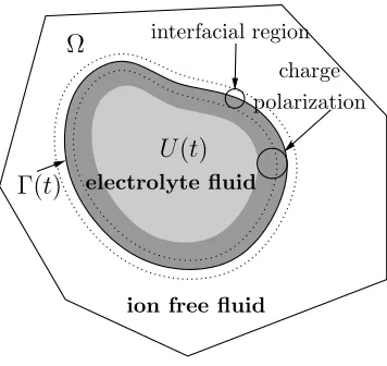
Ω
U(t) Γ(t)
charge polarization interfacial region
electrolyte fluid
[image:28.612.235.413.59.227.2]ion free fluid
Figure 3.1. Two phase fluid model of electrolyte droplet.
tously formulated in the context of an interface and electrolyte system. In tradi-tional approaches, the interface is stationary and is considered part of the domain boundary,∂Ω. The electric properties of the material opposite the electrolyte with respect to the interface boundary are described by boundary conditions of the variables n, p and V. From a physical standpoint, one must take care in summa-rizing the electric properties of the interface and region exterior to the electrolyte by boundary conditions (see [48].) Further, in many cases it is desirable that the interface be mobile. Freely floating inclusions such as large colloids ([16]) or vesicle membranes ([38]) are two important examples where a moving interface is present in an electrolyte.
3.2
Phase field barrier functional
In this chapter we propose a strategy to model the electrolyte and inclusions as a mixture of two incompressible fluids. We view the region occupied by the elec-trolyte as a time dependent subregion U(t) of the domain Ω. The interface is the boundary of this subregion, Γ(t) := ∂U(t). To achieve this end, we employ a phase field representation of the subregion U(t) by assigning
U(t) :={φ <0}, Γ(t) := {φ= 0} (3.1)
whereφ : Ω×[0, T]→R is the phase field indicator function. The phase field has an associated length scaleη which is the characteristic thickness of the interfacial region. The interfacial region is, roughly speaking, the region where φ is close to 0.
The intial data n0 and p0 of the variables n and p respectively are chosen so that the support of n0 and p0 are contained in U(0) = {φ(t = 0) < 0}. The ions are, however, diffuse, and will tend to migrate to the exterior ofU(t) as the system evolves. To ensure that this is not the case, we employ the following penalty formulation. We introduce the phase field barrier functional
BM(φ, n, p) :=
Z
Ω
M(φ+ 1)(n+p)dx. (3.2)
Owing to the special feature of the phase field function, φ is close to −1 in U(t) and 1 in the exterior ofU(t),
lim
η→0BM(φ, n, p) =M
Z
Ω\U(t)
n+p dx. (3.3)
Ideally, ifBM(φ, n, p) remains bounded independently oft andM, then n=p= 0 in Ω\U(t) asM → ∞.
Figure 3.2. Finite element simulation of droplet coalescence
energy and the mixing energy of the barrier potential. The mixing energy is of order M while the electric energy is of order ǫ−1/2. To ensure that the barrier potential energy is stronger than the electric energy, M is chosen larger than the electric energy scale. In simulation we consider the regime
η≪ǫ1/2 ≪Re, M−1 ≪ǫ1/2. (3.4)
The choice of the barrier functional (3.2) was motivated by the following Proposition 1. Suppose that v is divergence free and cand b satisfies
ct+v· ∇c= ∆c+M∇ ·(c∇b)
bt+v· ∇b = 0
where initially R
Ωc0b0dx= 0, c0 >0 and c|∂Ω = exp(−M) and b|∂Ω = 1. Then
Z
Ω
cb dx≤M−1 Z
Ω
colog(c0)dx+e−1|Ω|
Proof. Consider the energy densityA(c) =clog(c)+Mcb.By maximum principles,
c(x, t)≥0 for allx∈Ω and allt∈[0, T].Hence,A(c) is always defined. Note that
Ac = 1 + log(c) +Mb and ∇Ac =c−1∇c+M∇b. A brief calculation then shows that
d dt
Z
Ω
A(c)dx=−
Z
Ω
c|∇Ac|2dx. (3.5)
(3.5) simply says thatR
ΩA(c)dx is decreasing in time. Consequently
Z
Ω
A(c)dx≤ Z
Ω
A(c0)dx=
Z
Ω
c0log(c0)dx.
For c >0, we have that clog(c)> −exp(−1). Bounding the leftmost term in the above inequality from below, we find
−e−1|Ω|+M Z
Ω
cb dx≤ Z
Ω
c0log(c0)dx.
The above proposition states that in the ideal case when the indicator function
b is transported, the integral (mass) of the density functioncover the preimage of the value ofbgreater than any number is bounded uniformly in time. This integral can be made arbitrarily small for all time by chosing M large.
The barrier functional can further be motivated by considering the potential energy as due to shorter range interactions than the usual inverse distance elec-trostatic interaction. Assuming x is sufficiently far from the boundary of Ω, we formaly write
φ(x) =
Z
Ω 1
|x−y|∆φ(y)dy≈ Z
Ω\U(t)
2d−2 |x−y|3 dy
3.3
A model of electrolyte droplets
We consider the following system of the hydrodynamic flow of two incompressible fluids; the first fluid is an electrolyte, while the second fluid ion free; it has no or very little ions.
ρ(ut+u· ∇u) +∇π =ν∆u+ (n−p)∇V − ∇ ·(∇φ⊗ ∇φ), (3.6)
∇ ·u= 0, (3.7)
nt+u· ∇n=∇ ·(Dn∇n−µnn∇V +Mn∇φ), (3.8) pt+u· ∇p=∇ ·(Dp∇p+µpp∇V +Mp∇φ), (3.9)
∇ ·(ǫ∇V) =n−p, (3.10)
φt+u· ∇φ =γ(∆φ−η−2W′(φ)) (3.11)
Equations (3.6) and (3.7) are the Navier-Stokes (NS) equations whereu is the fluid velocity of the electrolyte fluid, π is the pressure, ρ is the fluid density and
ν the fluid viscocity. In equation (3.6), (n−p)∇V is the macroscopic Lorentz (or Coulomb) force. Similarly, ∇ ·(∇φ⊗ ∇φ) approximates the surface tension of the interface, see [37].
Equations (3.8) and (3.9) are the Nernst-Plank equations of a binary charge system, n and p are the densities of diffuse, negative and positive charges respec-tively. Dn, Dp are the respective diffusivity constants andµn, µp are the respective mobility constants. µn, µp and Dn and Dp are related by Einstein’s relation and the valence of the charged bodies. For example, in a solution of potassium chloride (KCl), the negative and positive valences are 1, (Cl−,K+). In equations (3.8) and (3.9) the convection involving ∇V is the migration of charge bodies due to the microscopic Coulomb’s force experienced by the charged bodies in the direction of the electric field (−∇V). The convective termM∇φ in (3.8) and (3.9), as we will see later, is derived from the mixing energy (3.2).
of the transport equation
φt+u· ∇φ = 0.
In this chapter we simply let ρ = Dn = Dp = µn = µp = 1. We consider the case when
u
∂Ω = 0, n|∂Ω =f >0, p|∂Ω =g >0, (3.12)
V
∂Ω =V0, φ
∂Ω = 1. (3.13)
3.4
Free energy variation
In this section we derive equations (3.6)-(3.11) from a free energy using variational principles. We define the internal energy of the electrolyte-interface system
L(n, p) =
Z
Ω
nlog(n) +plog(p) +V(p−n)dx
+BM(φ, n, p) +Sη(φ).
(3.14)
HereV is a solution of the Poisson equation (3.10) and thus may written explicitly in terms of convolution with the Green’s kernel G(x, y).
V(x) =
Z
Ω
G(x, y)
2ǫ (n(y)−p(y))dy.
We may rewrite (3.14)
L(n, p) =
Z
Ω
nlog(n) +plog(p)dx
+
Z Z
Ω2
G(x, y)
2ǫ (n−p)(y)(n−p)(x)dy dx
+BM(φ, n, p) +Sη(φ).
(3.15)
BM(φ, n, p) was defined in (3.2) and
Sη(φ) =
Z
Ω
η
2|∇φ| 2+ 1
4η(φ
2
In this form, we see that the free energy (3.15) is composed of entropic contribu-tions (the logarithmic terms), electrostatic interaction (Green’s kernel), the barrier functional and the interface surface area.
We define the chemical potentialβ(n) andβ(p) as the usual Frechet derivatives of L with respect ton and prespectively;
β(n) = 1 + log(n)−V +M(φ+ 1),
β(p) = 1 + log(p) +V +M(φ+ 1). (3.17)
The fluxes J(n) and J(p) are defined as the gradient of β(n) and β(p), scaled by
n and p respectively (Fick’s Law);
J(n) =n∇β(n), J(p) =p∇β(p). (3.18)
If, in addition,nandpare macroscopically transported by the fluid velocity uand
J(n) and J(p) are the fluxes ofnandp, then the conservation of mass implies that
nt+u· ∇n=∇J(n), pt+u· ∇p=∇J(p). (3.19) In contrast, we will now show that (3.18) and (3.19) are also variational in structure. We elaborate briefly. n and p are both a number density correspond-ing to the position of the negative and positive ions (particles) respectively. In particular, n and p can be written in terms of the inverse Jacobian of the map which specifies the position of these particles. The only variation which can occur in the physical system is with respect to the particle positions. This variation cor-responds to the usual variation of the function, where the function is the particle position map. Suppose that the particle positions are perturbed by the field v.
It is not hard to check that the deviation ns and ps of n and p respectively then
satisfy
δns+∇ ·(nsv) = 0, δps+∇ ·(psv) = 0, n0 =n, p0 =p.
n; d ds
s=0L(n
s, p) =
−
Z
Ω
β(n)∇ ·(nv)dx
=
Z
Ω
nv· ∇β(n)dx=
Z
Ω
nv·
∇n n − ∇V
dx
=
Z
Ω
v·J(n)dx
We see that the flux J(n) is the microscopic force experienced by the particle system. Because the motion of the particles is damped by fluid, the sum of micro-scopic forces J(n) translates into convection (net particle velocity.) Furthermore, if we define a variational derivative δL/δn of L by
Z
Ω
δL
δnw dx=− d ds
s=0L(n
s, p),=Z
Ω
J(n)· ∇w dx
∀w∈C0∞(Ω)
(3.20)
where∇wreplacesvin (3.20), we see that (3.8) is a transported, gradient descenct equation nt+u· ∇n = −δL/δn where the gradient direction is defined directly above. Analogous considerations hold for equation (3.9) and the variable p.
3.5
Verification for transport case
We will now study smooth solutions of (3.6-3.11) in the case when the phase field is purely transported, i.e. γ = 0.We will reproduce a similar result to Proposition 1. The difference here is that in addition to transport limited diffusion found in Proposition 1, the system (3.6-3.11) has the additional internal electrostatic coupling.
Suppose thatu,n,p, andφare C1 in time andC2 in space and solve (3.6-3.11) with initial data satisfying
n0 >0, p0 >0,
Z
Ω
(φ0+ 1)(n0+p0)dx= 0.
particular, no far electric fields may be present, i.e. V0 = constant. (3.6-3.11) are invariant under translations of the Dirichlet data forV. We thus choose
V0 = 0. (3.21)
Furthermore, we require that the chemical potential β(n) and β(p) vanish at the boundary;
n
∂Ω = exp(1−2M), p
∂Ω = exp(1−2M). (3.22) This implies that n, p > 0 on the boundary of Ω× [0, T]. A simple maximum principle then shows thatn and p are strictly positive in the interior as well.
Multiply equation (3.6) by the solution u and integrate by parts. One finds 1
2
d dtkuk
2
L2(Ω)+νk∇uk2L2(Ω) =
Z
Ω
(n−p)∇V ·u+ ∆φ∇φ·udx. (3.23)
Next, multiply (3.11) by ∆φ−W′(φ)/η2+M(n+p). Note thatW′(φ)∇φ is a total derivative;
d
dtSη(φ) + Z
Ω
Mφt(n+p) + ∆φ∇φ·u+M(n+p)∇φ·udx= 0 (3.24)
Finaly mutliply (3.8) by β(n) and (3.9) by β(p). Recall that β(n) = β(p) = 0 on∂Ω and (1 + log(c))∇cis a total derivative for c=n, p.
Z
Ω
(nt+u· ∇n)β(n)dx =
Z
Ω
(nlog(n))t+ (M(φ+ 1)−V)(nt+u· ∇n) =− Z
Ω
n|∇β(n)|2
(3.25)
Z
Ω
(pt+u· ∇p)β(p)dx=
Z
Ω
(plog(p))t+ (M(φ+ 1) +V)(pt+u· ∇p) =− Z
Ω
p|∇β(p)|2
(3.26)
where the right hand sides above come from integration by parts. Also, (n−p)Vt = ∆V Vt and (V0)t= 0 so that
Z
Ω
(p−n)Vtdx=− Z
Ω
∆V Vt = d dt
Z
Ω 1 2|∇V|
Summing (3.24)-(3.27), taking care account for the total derivatives
Z
Ω
M(φt+u· ∇φ)(n+p) +M(φ+ 1)(nt+pt+u· ∇(n+p))dx=
Z
Ω
M[(φ+ 1)(n+p)]t+u· ∇[(φ+ 1)(n+p)]dx
one finds
d
dtL(φ, n, p)−
1 2
d
dtk∇Vk
2
L2(Ω)
=−
Z
Ω
(n−p)∇V ·u+ ∆φ∇φ·udx
−
Z
Ω
n|∇β(n)|2+p|∇β(p)|2dx
(3.28)
Note that
k∇Vk2
L2(Ω) =
Z
∂Ω
V0∇V ·ndS− Z
Ω
(n−p)V dx
so that we may rewrite (3.28)
d
dtL˜(φ, n, p) =− Z
Ω
(n−p)∇V ·u+ ∆φ∇φ·udx
−
Z
Ω
n|∇β(n)|2+p|∇β(p)|2dx
(3.29) where ˜ L:= Z Ω
nlog(n) +plog(p) + 1
2V(p−n)dx+BM(φ, n, p) +Sη(φ) =L−1
2k∇Vk 2
L2(Ω).
Summing (3.29) with (3.23), we finally have
d dt(kuk
2
L2(Ω)+ ˜L) +νk∇uk2L2(Ω)≤0. (3.30) (3.30) is the canonical energy inequality associated with (3.6-3.11) and captures the dissipation of kinetic and internal energy. It implies that ku(t)k2
L2(Ω)+ ˜L(t)< ku(0)k2
˜
L(0) from above, then this inequaltiy implies
Z
Ω
(φ+ 1)(n+p)dx≤ M−1(2e−1|Ω|+c0), ∀t ∈[0, T].
This inequality is the same as found in Proposition 1. It is remarkable that it still holds despite the presence of a possible competing internal dynamic.
On solution existence
We will briefly discuss the existence of weak solutions to (3.6-3.11). Due to regular-ity considerations, it is necassary to assume thatγ >0.In this case, the procedure in the above section fails to produce an energy inequality of the form (3.30). This in part due to the fact that the variational structures which determine φ differs from that ofn and p.
Note that intrinsicly (3.30) is not a sufficient apriori estimate to produce a weak solutions to (3.8) and (3.9), as it implies thatn and p are only slightly more than integrable in space. Instead, depending on the regularity of φ, solutions of (3.8) and (3.9) satisfy a stronger energy inequality of the type usually derived for parabolic PDE. When φ solves (3.11), this stronger inequality holds for space dimension 2 and implies the existence of weak solutions for sufficiently small initial data. In summary, one may prove the following small data, global in time, existence theorem:
Theorem 1. Let Ω ⊂ R2 be bounded with smooth boundary. For kn0k
L2(Ω), kp0kL2(Ω) and k∇φ0kL2(Ω) sufficiently small, there exist a Leray solution of
(3.6-3.11) satifying boundary conditions (3.22) and (3.21).
The ability to construct a Galerkin approximate solution to (3.6-3.11) is highly dependent on the sign relationship between n,pandV and also the positivity ofn
and p. In general, positivity is difficult to ascertain for a Galerkin (or numerical) approximation, due to a lack of smoothness. However, one may prove the maximum principle, Lemma 4 found in the next chapter.
3.6
Simulation
We present several numerical simulations of equations (3.6-3.11). These simula-tions serve three purposes. The first is to demonstrate concretely the dynamic interaction between electrostatic, interfacial and fluid forces. The second is to ver-ify the potency of the phase field barrier functional, (3.2), in restricting densities to subregions of the domain. Finally, researchers traditionally avoid solving (3.6-3.11) numerically due to the boundary layer structure. Our algorthim, however, clearly preserves the boundary layer structure and resolves the Reynolds, Debye, and interfacial length scale without difficulty. Below we describe some of the fea-tures of this algorithm, in particular we elaborate on the finite elements used to discretize (3.6-3.11).
The following simulations were performed for a 1 by 1 unit square. The grid points were chosen uniformly with a mesh size of h = .01 We use Delaunay tri-angulations (generated by [53]) and a fully implicit forward Euler time stepping scheme with time step τ = 4×10⁻².
The viscocityνand Reynolds numberRewas 1. ηwas chosen as 10−2.Although
η is comparable to the mesh length h the interfacial region was clearly resolved, as is seen from the numerical experiments. The dielectricǫ was chosen to be 10−2. Thus η ≪ ǫ1/2 ≪ Re, as is desired by (3.4). A penalty coefficient of M = 5 was sufficient to almost entirely restrict the discrete densities to the droplet interior. This was suprising because the electric potential characteristically was only of one magnitude less. We chose γ = 10−3 so that the change in volume of the droplet did not signficanlty affect the dynamic of the simulation.
A simple iteration between equations (3.6)-(3.11) leads to a fixed point solution of the nonlinear couplings. We used Newton’s method to solve (3.11) for each time step.
defined by B3
T,h = λ1,Tλ2,Tλ3,T, where {λi}3i=1 are the barycentric coordinates associated with T. The pressure π was discretized by piecewise linear continuous elements. As it is well known, that the continuous, piecwise linear plus bubble velocity and continuous piecewise linear pressure is a stable finite element pair for the Stokes equation, namely, it satisfies the inf-sup condition [15], [17].
In our calculations, we have used a direct method to solve the Stokes equation since our problem was relatively small, of sizeO(104). However, for smaller values of the characteristic mesh sizeh, it will be necassary to use iterative methods. such as the Uzawa method [17], [54] and augmented Lagrangian algorithm [17].
At each time step, we discretize the operators in (3.8),(3.9) and (3.11) by the EAFE scheme proposed in [58]. The EAFE scheme is type of upwinding scheme for finite elements with automatic choice of the upwind direction. Such a dis-cretization is monotone for Delaunay triangulations, that is, the resulting stiffness matrix corresponding to the bilinear form of the convection diffusion equation, (with continuous convection and diffusion coefficients) is anM matrix if and only if the usual stiffness matrix corresponding to the Poisson equation is also an M
matrix. In the time stepping procedure, in the the fixed point iteration of the charge densities and during the Netwon iteration for the phase field, we must solve convection diffusion equations of the form
∇ ·(∇u+uβ) =f. (3.31)
0.0 0.1 0.2 0.3 0.4 0.5 0.6 0.7 0.8 1.50
1.75 2.00 2.25 2.50 2.75 3.00
t= time
Sη
(
φ
)
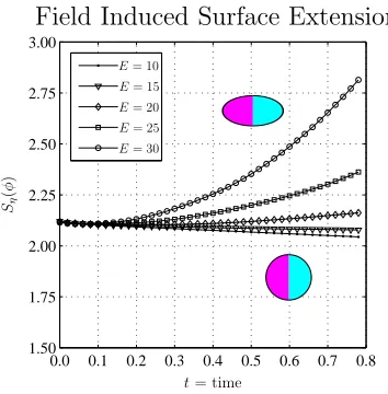
[image:41.612.223.400.47.227.2]E= 10 E= 15 E= 20 E= 25 E= 30
Figure 3.3. Evolution of phase field energySη(φ) for a variety of applied fields E.
Figure 3.4. Evolution of phase field for two oppositely charged droplets.
Field induced extension
The first class of simulations we present demonstrates the competition between electostatic forces and interfacial forces. We demonstrate this by applying an elec-tric field across an initially neutral electrolyte droplet by specifying the boundary conditions
V(x, y) = Ex, (x, y)∈∂([0,1]×[0,1]). (3.32)
φ was initially chosen so that U(0) was a ball centered at (1/2,1/2) and n and p
where chosen to be identically 0.5 in this ball and 0 outside this ball.
[image:41.612.220.434.274.409.2]w.r.t. the x = 1/2 axis and consequently stretch the droplet interface. For small fields the surface tension of the interface is sufficient to withstand the force induced by this polarization, and the droplet surface area decreases2. For large electric fields, the polarization induced force overcomes the surface tension and the surface area increases. Figure 3.3 compares this growth in surface area with respect to time for several different applied field strengthsE.We point out that from the energetic point of view, the system is converting electric energy fromE into surface energy
Sη(φ).
Charge induced coalescence
Next we consider two electrolyte droplets with opposite charge seperated over some distance.
φ is initially chosen so that U(0) is the union of two balls a distance apart.
n is initally chosen to be a constant 0.5 in the first ball, zero elsewhere and p is chosen to be 0.5 in the second ball and zero elsewhere. V satisfies zero boundary conditions.
The charge seperation produces a gradient in electric potential which in turn causes fluid motion through the Lorentz force. This causes the two seperated phases to move toward each other until they merge. The two phases coalesce at a close enough distance, widening the support of the negative charge density to that of the positive charge density and vic versa. The densities migrate into the other phase until a single, charge neutral phase is reached. At this point, interfacial forces dominate the motion of the phase and the droplet evolves under surface tension.
The dynamics of these two droplets are such that the electric energy is dissi-pated into kinetic energy in order to resolve the topological seperation. As the droplets are close enough, the energy of the topological seperation is lost. This can be seen in figure 3.6 as the sharp drop in surface energy Sη(φ).
Figures 3.5 and 3.6 clearly demonstrate the utility of our phase field barrier
2The phase field equation is not volume preserving in our simulation. Such a modification
0 1 2 3 4 5 6 7 0.1880 0.1882 0.1884 0.1886 0.1888 0.1890 0.1892 0.1894
0 1 2 3 4 5 6 7
0.0 0.2 0.4 0.6 0.8 1.0 1.2 1.4
t= time t= time
Negative Ion Mass InU(t)
R U(t)n dx
R
Ωn(1−φ)/2dx
Negative Ion Mass OutsideU(t)
R
Ω\U(t)n dx
R
Ωn(1 +φ)/2dx
×
10
−
[image:43.612.199.450.64.195.2]3
Figure 3.5. Mass conservation with respect toU(t)
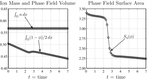
0 1 2 3 4 5 6 7
2.00 2.25 2.50 2.75 3.00 3.25 3.50
0 1 2 3 4 5 6 7
0.40 0.45 0.50 0.55 0.60 0.65
t= time t= time
Ion Mass and Phase Field Volume
R
Ωn dx
R
Ω(1−φ)/2dx
Phase Field Surface Area
Sη(φ)
Figure 3.6. Mass conservation in domain and change in surface energy
formulation. In figures 3.5 we see that the total density (mass) n interior to U(t) changes less than one hundreth of the total mass. Similarly, the mass exterior to droplet, despite diffusion and electric convection, is less than one hundreth of the total mass. Moreover, in figure 3.6, the total mass of n is almost constant in time while the phase field surface area Sη(φ) drops by 10% in the simulation time.
3.7
Conclusion
[image:43.612.204.444.235.363.2]formulation based on a barrier functional for restricting the support of solutions of the hydrodynamic Poisson-Nernst-Plank equations to the evolving subregions of the domain. We validated the model by energetic arguments and several dynamic, finite element simulations.
Future work will include modeling cell membranes by interfaces with elastic bending energy and spontaneous curvature [25], [26], as well as variable perme-abilities of the interface to ions [24], [40]. With an elastic interface, a particulary interesting application of our formulations would be to electric cell lysis, [38].
Classical and Weak Solutions
4.1
Preliminaries
We introduce the usual notation and spaces associated with the Navier-Stokes and other second order, time dependent equations. The inner product of two functions
u and v in L2(Ω) and two functions u and v in (L2(Ω))2 is denoted by (u, v) and (u,v) respectively. V is the space {v ∈(C∞
0 (Ω))3 : ∇ ·v= 0} and H and V are the closure of V in L2(Ω) and H1
0(Ω) respectively. We choose a basis {vi}∞i=1 for
H which satisfies (vi,vj) = δij and (∇vi,∇vj) = 0 if i 6= j (see [54].) we define
the forms
b(u, v, w) =
Z
Ω
u· ∇vw dx, b(u,v,w) = 3
X
i=1
b(u,vi,wi)
for all v, w ∈ H1(Ω) and u,v,w ∈ (H1(Ω))2. In three space dimensions, b and b are continuous and trilinear with respect to the H1
0(Ω) norm. Using the same notation, we will consider maps from [0, T] ⊂ R into the spaces X, whose norms are bounded in Lp for 1≤p≤ ∞. For example, Lp([0, T];X) (also writtenLp(X)
when the interval of dependence is clear) is defined as
u: [0, T]→X :
Z T
0 k
The space Y(α1, α2;X1, X2) is space of maps u∈Lα1(X1) withu′ ∈Lα2(X2). QT
is the cylinder Ω×[0, T]. We will frequently use Lemma 1. For u∈H1
0 and Ω∈R3 bounded with smooth boundary kukL4(Ω) ≤ kuk1/4
L2(Ω)kuk 3/4
H1
0(Ω). (4.1)
We define a second trilinear form, θ(u, f, v) for u, f ∈ H1(Ω), v ∈ H1 0(Ω) as follows,
θ(u, f, v) =
Z
Ω∇ ·
(u∇W)v dx=−
Z
Ω
u∇W · ∇v dx,
whenever ∆W = f with W|∂Ω = 0. With f ∈H1(Ω), W is differentiable so that the above integrals make sense. Furthermore, one has
Lemma 2. If u, f ∈H1(Ω) and v ∈H1
0(Ω), then
|θ(u, f, v)| ≤ c0kukH1(Ω)kfkH1(Ω)kvkL2(Ω), (4.2) |θ(u, f, v)| ≤ c2kukL2(Ω)kfkH1(Ω)kvkH1
0(Ω). (4.3)
for some constantsc0 andc2 depending only onΩ.Furthermore, ifu∈H01(Ω)then
θ(u, f, u) =
Z
Ω 1 2u
2f dx. (4.4)
Proof. By elliptic regularity, W ∈ C1(Ω) with k∇Wk
C0(Ω) ≤ c0kfkH1(Ω) for some
c0 =c0(Ω) when d≤3.Then
|θ(u, f, v)|=
Z Ω
u∇W · ∇v dx
≤
c0kukL2(Ω)k∇vkL2(Ω)kfkH1(Ω)
This implies (4.3). Also
|θ(u, f, v)|=
Z Ω
(∇u∇W +u∆W)v dx = Z Ω
(∇u∇W +uf)v dx
≤c0k∇ukL2(Ω)kvkL2(Ω)kfkH1(Ω)+kukL4(Ω)kfkL4(Ω)kvkL2(Ω) ≤c1kukH1(Ω)kfkH1(Ω)kvkL2(Ω)
(4.5)
For (4.4),
θ(u, f, u) = −
Z
Ω
u∇W∇u dx=−
Z
Ω 1 2∇u
2
∇W dx=
Z
Ω 1 2u
2f dx.
4.2
Classical Solutions to PNP Equations
Settingǫ=M = 1, we rewrite (3.8)-(3.10) in the following form
nt=∇ ·(∇n+n(∇φ− ∇V −u)), pt=∇ ·(∇p+p(∇φ+∇V −u)),
∆V =n−p.
This motivates the following
Theorem 2. Let n0, p0 ∈ C∞(Ω) and β1, β2 ∈ C∞(QT) and k > 0 a constant.
Then there exists unique, positive n, p ∈ C∞(Q
T) satisfying n, p|∂Ω = k for all
t∈[0, T], n, p|t=0=n0, p0 and
nt=∇ ·(∇n+n(β1 − ∇V)), (4.6)
pt =∇ ·(∇p+p(β2+∇V)), (4.7)
∆V =n−p. (4.8)
Theorem 2 is nontrivial in the sense that if one were to switch the sign of V, i.e. V solves ∆V =p−n, then [22] have shown that finite time blow-up solutions exist for sufficiently large initial data. We show in lemma 3 that (4.6)-(4.8) has a small time weak solution, in lemma 4 that this solution is positive and then extend the solution globally.
Lemma 3. Assume the hypothesis of theorem 2. Then there exist
˜
n,p˜∈Y([0, δ); 2,1;H01(Ω), H−1(Ω))