Abstract—The purpose of this paper is to study the Legendre wavelets for the solution of linear and nonlinear fractional integro-differential equations. The properties of Legendre wavelets together with the fractional order operational matrix of integration are used to reduce the problem to the solution of a system of algebraic equations. Also a reliable approach for convergence of the Legendre wavelets method is discussed. Further some numerical examples are shown to illustrate the accuracy and reliability of the proposed approach and the results have been compared with the exact solution.
Index Terms—Legendre wavelets, Block pulse functions, operational matrix, fractional integro-differential equation, convergence, numerical solution
I. INTRODUCTION
N recent years, fractional calculus has attracted many researchers successfully in different disciplines of science and engineering. One of the main advantages of the fractional calculus is that the fractional derivatives provide a superior approach for the description of memory and hereditary properties of various materials and processes [1-3]. Differential equations involving fractional order derivatives are used to model a variety of systems, such as the field of viscoelasticity, heat conduction, electrode-electrolyte polarization, electromagnetic waves, diffusion equations and so on [4-6]. Since its tremendous applications in several disciplines, a considerable attention has been given to the exact and the numerical solutions of fractional differential equations and fractional integral equations. Even numerical approximation of fractional differentiation of rough functions is not easy as it is an ill-posed problem.
Other than modeling aspects of these differential equations, the solution techniques and their reliability are rather more important. In order to obtain the goal of highly accurate and reliable solutions, several methods have been proposed to solve the fractional order differential and fractional order integral equations. The most commonly used methods are Variational Iteration Method [7], Adomian Decomposition Method [8-9], Generalized Differential Transform Method [10-11] and Wavelet Method [12-13].
Manuscript received August 4, 2017; revised March 06, 2018. Na Guo is with the Institute of Disaster Prevention, Sanhe, Hebei, P.R.China (e-mail: [email protected]).
Yunpeng Ma (Corresponding author) is with the School of Aeronautic Science and Engineering, Beihang University, Beijing, P.R.China (e-mail: [email protected]).
In this paper, the main objective of the present paper is to introduce the Legendre wavelets method to solve the linear and nonlinear fractional integro-differential equations. The method is based on reducing the equation to a system of algebraic equations by expanding the solution as Legendre wavelets with unknown coefficients. The main characteristic of an operational method is to convert a differential equation into an algebraic one. It not only simplifies the problem but also speeds up the computation.
II. LEGENDRE WAVELETS AND THEIR PROPERTIES The Legendre wavelets
nm( )
x
are given by the following [14]1/ 2
2 ˆ ˆ
2 1 ˆ 1 1
2 (2 ),
( ) 2 2 2
0,
k k
m k k
nm
m n n
P x n x
x
otherwise
(1)
where
k
1, 2,
,
n
ˆ 2
n
1
,n
1, 2,
, 2
k1 ,0,1,
,
1
m
M
is the degree of the Legendre polynomials andM
is a fixed positive integer,P x
m( )
are the Legendre polynomials of degreem
.A function
f x
( )
defined over[0,1)
may be expanded by the Legendre wavelets as1 0
( )
nm nm( )
n m
f x
c
x
(2)where
c
nm
f x
( ),
nm( )
x
, and,
is the inner product off x
( )
and
nm( )
x
.If the infinite series in Eq.(2) is truncated, then Eq.(2) can be written as
1
2 1
1 0
( )
( )
( )
k M
T nm nm
n m
f x
c
x
C
x
(3)where
C
and
( )
x
areˆ
2
k 1m
M
column vectors, given by1 1
10 1 1 2 0 2 1
[
,
,
,
,
k,
,
k]
TM M
C
c
c
c
c
(4)1 1
10 1 1 2 0 2 1
( )
[
,
,
,
,
k,
,
k]
TM M
x
(5)For simplicity, we write Eq.(5) as ˆ
1
( )
( )
( )
m
T i i
i
f x
c
x
C
x
(6)Numerical Algorithm to Solve Fractional
Integro-Differential Equations Based on
Legendre Wavelets Method
Na Guo and Yunpeng Ma*
I
IAENG International Journal of Applied Mathematics, 48:2, IJAM_48_2_06
where
c
i
c
nm,
i
nm. The indexi
is determined by the relationi
M n
(
1)
m
1
. Therefore, we have1 ˆ
1 2 (2 1) 1
[ ,
,
,
,
,
k,
,
]
T
M M m
C
c c
c
c
c
(7)1 ˆ
1 2 (2 1) 1
( )
[
,
,
,
,
,
k,
,
]
T
M M m
x
(8)Similarly, an arbitrary function of two variables
u x y
( , )
defined over[0,1) [0,1)
may be expanded into the Legendre wavelets basis asˆ ˆ 1 1
( , )
( )
( )
( )
( )
m m
T ij i j
i j
u x y
u
x
y
x U
y
(9)where
U
[
u
ij]
andu
ij
i( ),
x
u x y
( , ),
j( )
y
.We investigate the convergence of the Legendre wavelets expansion in the following theorems.
Theorem 2.1 A function
f x
( )
, defined on[0,1]
, is with bounded second derivative, sayf
( )
x
M
, can be expanded as an infinite sum of Legendre wavelets, and the series converges uniformly to the functionf x
( )
, that is1 0
( )
nm nm( )
n m
f x
c
x
,where
c
nm
f x
( ),
nm( )
x
and,
is the inner product off x
( )
and
nm( )
x
.Proof.
1 0
1/ 2 ˆ
( 1)/ 2
2 ˆ
( 1)/ 2
( )
( )
2
1
ˆ
( )
2
(2
)
2
k k nm nm k n k m nc
f x
x dx
m
f x
P
x
n dx
,let
2
kx
n
ˆ
t
, then1/ 2 1 2 1 1/ 2 1 1 1 1/ 2 1 1 1 1 1 1/ 2 1 1 1
ˆ 2 1 1
2 ( )
2 2 2
ˆ 2 1 ( ) 2 2 ˆ 1 ( ( ) ( ))
2 (2 1) 2
ˆ 1
( ( ) ( ))
2 (2 1) 2
k
nm k m k
m k k m m k k m m k k
n t m
c f P t dt
m n t
f P t dt
n t
f d P t P t
m
n t
f P t P t
m
1 1 1/ 2 1 1 1 1 1 ˆ 1 1 ( ( ) ( ))2k (2 1) 2k 2k m m
n t
f P t P t dt
m
1/ 2 1 1 13 1 1
1/ 2 1
2 2
3 1 1
1/ 2 2 3 1 ˆ 1 ( ( ) ( )) 2 (2 1) 2
ˆ ( ) ( ) ( ) ( ) 1
2 (2 1) 2 2 3 2 1
ˆ ( ) ( ) 1
2 (2 1) 2 2 3
m m
k k
m m m m
k k
m m m
k k
n t
f P t P t dt
m
P t P t P t P t
n t
f d
m m m
P t P t P
n t f m m
1 2 1 1/ 2 1 2 25 1 1
1/ 2 1
2 2
5 1 1
( ) ( ) 2 1 ˆ ( ) ( ) ( ) ( ) 1
2 (2 1) 2 2 3 2 1
ˆ ( ) ( ) ( ) ( ) 1
2 (2 1) 2 2 3 2 1
m m m m m
k k
m m m m
k k
t P t
m
P t P t P t P t
n t
f dt
m m m
P t P t P t P t
n t
f dt
m m m
Consider 2 1 2 2 1 2 1 2 2 1 2 1 2 2 1ˆ ( ) ( ) ( ) ( )
2 2 3 2 1
ˆ (2 1) ( ) (4 2) ( ) (2 3) ( )
2 (2 3)(2 1)
ˆ (2 1) ( ) (4 2) ( ) (2 3) ( )
2 (
m m m m k
m m m
k
m m m
k
P t P t P t P t
n t
f dt
m m
m P t m P t m P t
n t
f dt
m m
m P t m P t m P t
n t f dt
2 1 12 2 2 2 2 2
1
2 2 2
2 2
1 2
2 2 2
2 2
2 2
2 2
2 2
2 3)(2 1) (2 1) ( ) (4 2) ( ) (2 3) ( ) 2
(2 3) (2 1)
2 2 2 2
(2 1) (4 2) (2 3)
(2 3) (2 1) 2 5 2 1 2 3
2 12(2 3) (2 3) (2 1) 2 3
24 (2 1) (2
m m m
dt
m m
m P t m P t m P t
M dt
m m
M
m m m
m m m m m
M m
m m m
M m m
3) Thus, we obtain1
2 2
1
1/ 2
ˆ ( ) ( ) ( ) ( )
2 2 3 2 1
24
(2 1)(2 3)
m m m m
k
P t P t P t P t n t f dt m m M m m
.Therefore, we have
5 1 1
2 2 2
5 2
2
5 2
2
12 1 1
2 (2 1) (2 1)(2 3)
12 1 (2 3) 2 12 1 (2 3) (2 ) nm k k M c
m m m
m m n . Hence, the series
1 0 nm n m
c
is absolute convergent, itfollows that 1 0
( )
nm nm n mc
x
converges to the functions( )
f x
uniformly.Theorem 2.2 If a continuous function
u x y
( , )
defined on[0,1) [0,1)
has bounded mixed fourth partial derivative4 2 2
( , )
ˆ
u x y
M
x y
, then the Legendre wavelets expansion of( , )
u x y
converges uniformly to it.Proof. Let
u x y
( , )
be a function defined on[0,1] [0,1]
and4 2 2
( , )
ˆ
u x y
M
x y
, whereM
ˆ
is a positive constant. The Legendre wavelet coefficients of functionu x y
( , )
are defined as 1 1 0 0 1/ 2 1 / 2 0 ( , ) ( ) ( )2 1 ˆ
( , ) 2 (2 ) ( )
2
nk
ij i j
k k
m j
I
u u x y x y dxdy m
u x y P x n y dxdy
,by change of
2
kx
n
ˆ
t
, and1
2
kdx
dt
, we getIAENG International Journal of Applied Mathematics, 48:2, IJAM_48_2_06
1/ 2 1 1 / 2 0 1 1/ 2 1 1 1 1
1 0 1
1/ 2
1 1
1 1
1 0 1
ˆ 2 1
2 ( ) , ( )
2 2
ˆ 1
( ) , ( ( ) ( ))
2 (2 1) 2
ˆ 1
( ) , ( ( ) ( ))
2 (2 1) 2
k
ij j k m
j m m
k k
j m m
k k
m n t
u y u y P t dtdy
n t
y u y d P t P t dy
m
n t
y u y P t P t dy
m 1/ 2 1 1 1 1
1 0 1
1/ 2 1 1
1 1
3 1 0 1
1/ 2 1
3 1 1
ˆ ,
1 2 1
( ) ( ( ) ( ))
2 (2 1) 2
ˆ ,
1 2
( ) ( ( ) ( )) 2 (2 1)
ˆ ,
1 2
= ( )
2 (2 1)
k
j m m
k k
k
j m m
k k j k n t u y
y P t P t dtdy
m t
n t
u y
y P t P t dtdy
m t n t u y P y d m t 1 2 2 0 2 1/ 2 1 1 2 2
5 1 0 1 2
( ) ( ) ( ) ( )
2 3 2 1
ˆ ,
( ) ( ) ( ) ( )
1 2
( )
2 (2 1) 2 3 2 1
m m m m k
m m m m j
k
t P t P t P t
dy
m m
n t
u y
P t P t P t P t
y dtdy
m t m m
Now, let 2 2
( ) (2 1) ( ) 2(2 1) ( ) (2 3) ( )
m t m Pm t m P tm m Pm t
,then we have
1/ 2 5 1 2 1 1 2 0 1 1
2 (2 1)
ˆ ,
1 2
( ) ( )
(2 1)(2 3)
ij k k j m u m n t u y
y t dtdy
m m
t
.By solving this equation, we have 4 1 1 2 2 1 1 ˆ ˆ , 2 2 ( , ) ( ) ( ) k k
ij m m
n t n s u
u A k m t s dtds
t s
,where
( , )
5 11
21
22
k(2
1) (2
1) (2
3)
A k m
m
m
m
.So we have
4 1 1 2 2 1 1 ˆ ˆ , 2 2 ( , ) ( ) ( ) k k
ij m m
n t n s
u
u A k m t s dtds
t s
.Thus, we have
2
5 2
5 4
ˆ
24
(2
3)
( , )
2
3
1
1
2 (2
1) (2
3)(2
1)
ˆ
12
(2 ) (2
3)
ijk
M
m
u
A k m
m
m
m
m
M
n
m
.This means that the series 0 0 ij i j
u
is absolutelyconvergence.
III. OPERATIONAL MATRIX OF THE INTEGRATION FOR LEGENDRE WAVELETS
A. Fractional calculus
Before we introduce the Legendre wavelets operational matrix of the fractional integration, we first review some
basic definitions of fractional calculus, which have been given in [15].
Definition 1. The Riemann-Liouville fractional integral operator
J
of order is given by1 0
1
( )
(
)
( )
,
0
( )
xJ f x
x
f
d
(10)0
( )
( )
J f x
f x
(11) Definition 2. The Caputo definition of fractional differential operator is given by* ( ) 1 0 ( ) , ; ( )
1 ( )
, 0 1 .
( ) ( ) r r r x r
d f x
r N dx
D f x
f
d r r
r x
(12)The Caputo fractional derivatives of order
is also definedas
D f x
*( )
J
rD f x
r( )
. The relation between theRiemann-Liouville operator and Caputo operator are :
*
( )
( )
D J f x
f x
(13)1 ( ) *
0
( )
( )
(0 )
,
0
!
k r k kx
J D f x
f x
f
x
k
(14)B. Fractional order Legendre wavelets operational matrix of integration.
In this part, we may simply introduce the operational matrix of fractional integration of Legendre wavelets, more detailed introduction can be found in the Ref. [14].
Apart from the Legendre wavelets, we consider another basis set of block pulse functions. The set of these functions, over the interval
[0,1)
, is defined as [16]1,
(
1)
( )
0,
,
i
ih
x
i
h
b x
otherwise
i
0,1, 2,
,
m
ˆ
1
(15) with a positive integer value form
ˆ
and1
ˆ
h
m
.The following properties of block pulse functions will be used in this paper
0,
( ) ( )
( ),
i j ii
j
b x b x
b x
i
j
(16)1 0
0,
( ) ( )
1
,
ˆ
i j
i
j
b x b x dx
i
j
m
(17)Let
( )
[ ( ), ( ),
0 1,
ˆ 1( )]
T mB x
b x b x
b
x
. We suppose
( )
( )
J
B x
F B x
(18) whereF
is called the block pulse operational matrix of fractional integration [16], hereˆ
1 2 1
ˆ 1 2 ˆ 3 1 0 1 1
0 0 1
( 2)
0 0 0 1
m
m
m
F h
and1 1 1
(
1)
2
(
1)
k
k
k
k
,
k
1, 2,
,
m
ˆ
1
.IAENG International Journal of Applied Mathematics, 48:2, IJAM_48_2_06
There is a relation between the block pulse functions and Legendre wavelets, namely
( )
x
B x
( )
(19) where
[ ( ),
x
0
( ),
x
1,
mˆ1]
,ˆ
ii
x
m
,ˆ
0,1,
,
1
i
m
.If
J
is fractional integration operator of Legendre wavelets, we can get:( )
( )
J
x
P
x
(20) whereP
is called the Legendre wavelets operational matrix of fractional integration. Using Eq.(18) and Eq.(19), we have( )
( )
( )
( )
J
x
J
B t
J B t
F B t
(21) From Eq.(20) and Eq.(21), we can obtain( )
( )
( )
P
x
P
B x
F B x
(22)Then, the matrix
P
is given by 1P
F
(23) IV. THE ALGORITHM FOR FINDING NUMERICAL SOLUTION OFFRACTIONAL INTEGRO-DIFFERENTIAL EQUATIONS
A. Linear multi-order fractional integro-differential equations
Consider the linear multi-order fractional integro- differential equations
* *
1
1
1 0 1 2 0 2
( )
( )
( )
( , ) ( )
( , ) ( )
( )
i
r i i
x
a x D y x
D y x
k x t y t dt
k x t y t dt
f x
(24)
subject to initial conditions ( )
(0)
0,
0,1,
,
1
sy
s
(25) where
1
2
r ,D
* denote the Caputo fractional order derivative of order
,a x
i( )
is known function,
is the ceiling function,f x
( )
is input term andy x
( )
is the output response.k x t k x t
1( , ),
2( , )
are given functions.
1,
2are real constants.Now we approximate
D y x k x t k x t
*( ),
1( , ),
2( , )
and
( )
f x
in terms of Legendre wavelets as follows *1 1
2 2
( )
( ),
( , )
( )
( ),
( , )
( )
( )
T T T
D y x
C
x
k x t
x K
t
k x t
x K
t
(26)
and
( )
T( )
f x
F
x
(27) whereK
1
[
k
ij m m1]
ˆ ˆ,
K
2
[
k
ij m m2]
ˆ ˆ andˆ 1 2
[ ,
,
m]
TF
f f
f
. A similar approximation scheme is follow for variable coefficienta x
i( )
as well.Let
ˆ( )
i T( )
i m
a x
A
x
(28) where ˆi m
A
is knownm
ˆ 1
column vector.Now using Eq.(23) and (26) together with above approximation of
a x
i( )
, we obtain
*
( )
*( )
( )
( )
i i
i
i
T T
D y x
J
D y x
J
C
x
C P
x
(29)
and
( )
T( )
T( )
y x
C P
x
C P
B x
(30) Let[ , ,
0 1,
ˆ 1]
T m
E
e e
e
C P
, then1 0
1 0
1 0
1 0
1 1
( , ) ( )
( )
( )
( )[
]
( )
( )
( )
( )
( ) ( )
( )
( )
( )
( )
xx
T T T T
x
T T T
x T
T T
T
k x t y t dt
x K
t
t C P
dt
x K
B t B t E dt
x K
diag E B t dt
B
x
K
diag E F B x
Q B x
(31)
where
Q
is am
ˆ
-vector with elements equal to the diagonal entries of the following matrix1
1
( )
T
Q
K
diag E F
(32) and1 2 0
1
2 0
2
2
( , ) ( )
( )
( )
( )[
]
1
( )
[
]
ˆ
1
( )
ˆ
T T T T
T T T
T T
k x t y t dt
x K
t
t C P
dt
x K C P
m
C P K
B x
m
(33)
Substituting the above equations into Eq.(24), we have
ˆ1
1 2
2
( )
( )
[
]
( )
( )
( )
( )
ˆ
i
r T
i T T T
m i
T T
T T T
A
B x B
x
P
C
C
B x
Q B x
C P K
B x
F
B x
m
(34)
Define
[
]
[ , ,
0 1,
ˆ 1]
[
ˆ]
i
T T i i i T i T
m m
P
C
v v
v
V
, thenEq.(34) becomes
ˆ ˆ1
1 2
2
(
) ( )
( )
( )
( )
( )
ˆ
r T
i i
m m
i
T T
T T T
A
diag V B x
C
B x
Q B x
C P K
B x
F
B x
m
(35)
Dispersing Eq.(35), we get
IAENG International Journal of Applied Mathematics, 48:2, IJAM_48_2_06
ˆ ˆ 12
1 2
(
)
ˆ
r T
i i T
m m
i
T T T T
A
diag V
C
Q
C P K
F
m
(36)
which is a linear system of algebraic equations. By solving this system we can obtain the approximation of Eq.(30).
B. Nonlinear multi-order fractional integro-differential equations
In this section we deal with nonlinear multi-order fractional integro-differential equation of the form
* * 1 0 1
1 1
2 0 2
( )
( )
( )
( , )[ ( )]
( , )[ ( )]
( )
i
r x
p i
i
q
a x D y x
D y x
k x t y t
dt
k x t y t
dt
f x
(37)
subject to initial conditions ( )
(0)
0,
0,1,
,
1
sy
s
,where
p q
,
N
, and the other parameters and variables are the same as the section 4.1. While dealing with such a situation, the same procedure of expansion of fractional order derivatives via block pulse functions is adopted with exception at the term containing[ ( )] , [ ( )]
y t
py t
q.From Eq.(30), we have
y x
( )
EB x
( )
and henceˆ
0 1 1
[ ( )]
[
( )]
[
,
,
,
] ( )
( )
p p
p p p
m p
y t
EB t
e e
e
B t
E B t
(38)and
ˆ
0 1 1
[ ( )]
[
( )]
[ ,
,
,
] ( )
( )
q q
q q q
m q
y t
EB t
e e
e
B t
E B t
(39)Following the procedure of section 4.1and using the Eq.(38) and Eq.(39), the Eq.(37) is transformed into a nonlinear system of algebraic equations
ˆ ˆ1
2
1 2
(
)
ˆ
r T
i i T
m m
i
T T T T
q
A
diag V
C
W
E
K
F
m
(40)
where
W
is am
ˆ
-vector with elements equal to the diagonal entries of the following matrix1
1
(
)
T
p
W
K
diag E F
(41) Solving the system of equations given by Eq.(40), the approximate numerical solutiony x
( )
is obtained. The Eq.(40) can be solved by iterative numerical technique such as Newton’s method.V. NUMERICAL EXAMPLES
In order to illustrate the effectiveness of the proposed method, we consider numerical examples of linear and nonlinear nature.
Example 5.1. Consider the following linear equation:
2 1.5 0.5 1.7
1
0 0
( )
( )
( )
(
) ( )
(
) ( )
( )
xx D y x
xD y x
D y x
x t y t dt
x t y t dt
f x
(42)with this condition
y
(0)
y
(0)
0
and2.5
4 5
3.5 0.3 1.3
(3) (3) ( )
(1.5) (2.5)
(4) (4) (3) (4) 7 9
(2.5) (3.5) (1.3) (2.3) 12 20 12 20
f x x
x x x
x x x
.
The exact solution of this problem is
y x
( )
x
2
x
3. Table I shows the approximate solutions and exact solutions for differentk
,M
2
.TABLE I
THE APPROXIMATE SOLUTION AND EXACT SOLUTION FOR DIFFERENT
k
, M 2.x
k
4
k
5
k
6
k
7
Exact solution 0 0.000024 0.000012 0.000007 0.000000 0.00000 1/8 0.015822 0.016551 0.017198 0.017566 0.017578 2/8 0.075531 0.077098 0.077920 0.078115 0.078125 3/8 0.192880 0.193159 0.193317 0.193351 0.193359 4/8 0.361498 0.368505 0.373205 0.374988 0.375000 5/8 0.622950 0.626293 0.631080 0.634693 0.634765 6/8 0.930901 0.963194 0.981423 0.984162 0.984375 7/8 1.391340 1.408939 1.422946 1.434649 1.435546 From the Table I, we can see clearly that the numerical solutions are more and more close to the exact solution whenk
increases.Example 5.2. Consider this equation:
2 1.6 2 1.2 2 0.75
1 2.3
0 0
( 1) ( ) ( 1) ( ) ( )
1 1
( ) ( ) ( ) ( ) ( )
4 2
x
x D y x x D y x x D y x
D y x x t y t dt xty t dt f x
(43)where
3.9 1.9 4.3 2.3
5.5
4.75 1.2
(4.5)
(4.5)
( )
(
)
(
)
(2.9)
(3.3)
(4.5)
(4.5)
(3.75)
(2.2)
99
11
f x
x
x
x
x
x
x
x
x
,
such that
y
(0)
y
(0)
y
(0)
0
, the exact solution is 72
( )
y x
x
. The numerical results fork
3, 4,5, 6
,2
M
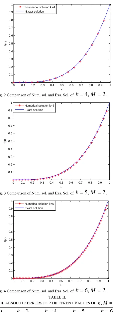
are shown in Figs.1-4. From the Figs.1-4, we can find easily that the numerical solutions are in good agreement with the exact solutions. The absolute errors for different values ofk
are shown in Table II. Through Table II, we can also see that the errors are smaller and smaller whenk
increases.
0 0.1 0.2 0.3 0.4 0.5 0.6 0.7 0.8 0.9 1
0 0.1 0.2 0.3 0.4 0.5 0.6 0.7 0.8 0.9 1
x
f(
x
)
Numerical solution k=3 Exact solution
[image:5.595.313.539.593.772.2]Fig. 1 Comparison of Num. sol. and Exa. Sol. of
k
3,
M
2
.IAENG International Journal of Applied Mathematics, 48:2, IJAM_48_2_06
0 0.1 0.2 0.3 0.4 0.5 0.6 0.7 0.8 0.9 1 0
0.1 0.2 0.3 0.4 0.5 0.6 0.7 0.8 0.9 1
x
f(
x
)
Numerical solution k=4 Exact solution
[image:6.595.54.280.48.672.2]Fig. 2 Comparison of Num. sol. and Exa. Sol. of
k
4,
M
2
.0 0.1 0.2 0.3 0.4 0.5 0.6 0.7 0.8 0.9 1 0
0.1 0.2 0.3 0.4 0.5 0.6 0.7 0.8 0.9 1
x
f(
x
)
Numerical solution k=5 Exact solution
Fig. 3 Comparison of Num. sol. and Exa. Sol. of
k
5,
M
2
.0 0.1 0.2 0.3 0.4 0.5 0.6 0.7 0.8 0.9 1 0
0.1 0.2 0.3 0.4 0.5 0.6 0.7 0.8 0.9 1
x
f(
x
)
Numerical solution k=6 Exact solution
Fig. 4 Comparison of Num. sol. and Exa. Sol. of
k
6,
M
2
. TABLE II.THE ABSOLUTE ERRORS FOR DIFFERENT VALUES OFk M, 2.
x
k
3
k
4
k
5
k
6
0 0 0 0 0
1/8 2.24755e-004 4.86626e-005 6.63916e-006 7.06361e-006 2/8 5.68826e-004 8.92015e-005 4.52890e-005 8.47627e-006 3/8 8.06345e-004 7.09312e-005 3.13733e-005 4.04433e-006 4/8 2.37124e-003 2.36345e-004 7.36812e-005 9.10813e-006 5/8 2.80843e-003 7.10940e-004 2.44000e-004 3.74311e-005 6/8 3.16123e-003 2.50721e-003 3.80861e-004 4.30647e-005 7/8 3.35997e-003 3.03684e-003 6.01802e-004 6.80648e-005
VI. CONCLUSIONS
In the present manuscript, the application and scope of the Legendre wavelets have been extended to fractional order linear and nonlinear integro-differential equations successfully. We construct fractional orders generalized Legendre wavelets operational matrix of integration and use this to solve the fractional linear and nonlinear integro- differential equations numerically. By solving the linear and nonlinear system, numerical solutions are obtained. The convergence analysis of Legendre wavelets is proposed. The numerical results show that the approximation is in very good coincidence with the exact solution.
REFERENCES
[1] J. C. Wang, “Realizations of generalized Warburg impedance with RC ladder networks and transmission lines,” Journal of the Electrochemical Society, vol.134, no. 8, pp. 1915-1920, 1987. [2] F. J. Valdes-Parada, J.A. Ochoa-Tapia, J. Alvarez-Ramirez, “Effective
medium equations for fractional Fick’s law in porous media,” Physical A, vol.373, pp. 339-353, 2007.
[3] H. Song, M.X. Yi, J. Huang, Y.L. Pan, “Numerical solution of fractional partial differential equations by using Legendre wavelets,”
Engineering Letter, vol. 24, no. 3 pp. 358-364, 2016.
[4] M. Ichise, Y. Nagayanagi, T. Kojima, “An analog simulation of noninteger order transfer functions for analysis of electrode process,”
Journal of Electroanalytical Chemistry, vol.33, pp. 253- 265,1971. [5] Z.M. Yan, F.X. Lu, “Existence of a new class of impulsive Riemann-
Liouville fractional partial neutral functional differential equations with infinite delay,” IAENG International Journal of Applied Mathematics, vol. 45, no. 4, pp.300-312, 2015.
[6] H. Song, M.X. Yi, J. Huang, Y.L. Pan, “Bernstein polynomials method for a class of generalized variable order fractional differential equations,” IAENG International Journal of Applied Mathematics, vol. 46, no.4, pp. 437-444, 2016.
[7] Z. M. Odibat, “A study on the convergence of variational iteration method,” Mathematical and Computer Modelling, vol.51, pp. 1181- 1192, 2010.
[8] I.L. EI-Kalla, “Convergence of the Adomian method applied to a class of nonlinear integral equations,” Applied Mathematics and Computation, vol.21, pp. 372-376, 2008.
[9] M.M. Hosseini, “Adomian decomposition method for solution of nonlinear differential algebraic equations,” Applied Mathematics and Computation, vol.181, pp. 1737-1744, 2006.
[10] S. Momani, Z. Odibat, “Generalized differential transform method for solving a space and time-fractional diffusion-wave equation,” Physics Letters A, vol.370, pp. 379-387, 2007.
[11] Z. Odibat, S. Momani, “Generalized differential transform method: Application to differential equations of fractional order,” Applied Mathematics and Computation, vol.197, pp. 467- 477, 2008. [12] Y. M. Chen, M. X. Yi, C. X. Yu, “Error analysis for numerical solution
of fractional differential equation by Haar wavelets method,” Journal of Computational Science, vol.5, no. 3, pp. 367-373, 2012.
[13] J. L. Wu, “A wavelet operational method for solving fractional partial differential equations numerically,” Appl. Math. Comput., vol.214 , pp. 31-40, 2009.
[14] H. Jafari, S.A. Yousefi, “Application of Legendre wavelets for solving fractional differential equations,” Computers and Mathematics with Application, vol.62, no.3, pp. 1038-1045, 2011.
[15] I. Podlubny, Fractional Differential Equations, Academic press, 1999. [16] Y.L. Li, N. Sun, “Numerical solution of fractional differential equations using the generalized block pulse operational matrix,”
Comput. Math. Appl., vol.62, pp. 1046 -1054, 2011.