A Generalization of the Exponential Function to
Model Growth
Martin Ricker and Dietrich von Rosen
Abstract—We generalize the exponential function to model instantaneous relative growth. The modified function is defined by a linear relationship between a continuous quantity (rather than time) and logarithmic relative growth. The corresponding formula is lnq
t q
t a b q t
, where
q t q t is instantaneous relative growth of a quantity q, t refers to time, a denotes initial logarithmic relative growth, and b is a shape parameter in terms of its sign, as well as a scaling parameter in terms of its magnitude. For calculating
q t , the exponential integral Ei
b q
exp
b q q q
d is needed. The problem of taking the inverse of Ei
x zEi is addressed. In order to distinguish two possible solutions for given zEi, we define the two inverse functions Ei( 1)x 0 zEi
and ( 1)
0 Eix zEi
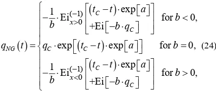
. An indirect method for their numerical evaluation is developed. With the generalized exponential function, one can model sigmoid growth (b0), exponential growth (b0), and explosive growth (b0), where the term “explosive growth” refers to a relative growth rate that increases with time. The resulting formula of generalized exponential growth is
( 1) 0 ( 1) 0
1
Ei exp +Ei for 0,
1
Ei exp +Ei for 0,
C C
C C
x
x
t t a b q b
b q t
t t a b q b
b
where qC is a calibrating quantity at time tC. For b0, the two functions equal the (standard) exponential function
C exp
C
exp
q t q tt a. In the case of sigmoid growth, the inflection point quantity is 1 /b, which depends only on one parameter (b). Negative growth can be modeled by substituting ttC with tCt. Any two points of logarithmic
relative growth can be connected unambiguously with the
Manuscript received on September 22, 2017; revised on April 18, 2018. The Dirección General de Asuntos del Personal Académico (DGAPA) of the Universidad Nacional Autónoma de México (UNAM) provided a stipend for the first author (MR), to spend a sabbatical year at the Swedish University of Agricultural Sciences in 2014-15.
M. Ricker is with the Instituto de Biología, Universidad Nacional Autónoma de México (UNAM), Mexico City (e-mail: [email protected], [email protected]).
D. von Rosen is with the Department of Energy and Technology, Swedish University of Agricultural Sciences, Uppsala, Sweden, as well as with the Department of Mathematics, Linköping University, Linköping, Sweden (e-mail: [email protected]).
generalized exponential function, to derive the corresponding function of q t
. Furthermore, we derive formulas for the conversion of a segmented curve of logarithmic relative growth as a function of time, into an equivalent growth curve of q t
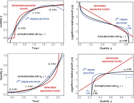
. Finally, the generalized exponential function is compared with a 2nd-degree polynomial and the nonlinear Schnute function. In conclusion, the generalized exponential function is useful for modeling a path of changing relative growth continuously, and to translate it into a growth curve of quantity as a function of time.Index terms - Exponential growth, Exponential function, Exponential integral Ei
x , Growth curves, Inverse of the exponential integral function, Explosive growth, Schnute function, Sigmoid growthI. INTRODUCTION
Growth curves are monotonically increasing functions over time. In the case of negative growth, they can also be monotonically decreasing functions. Growth curves are of interest in a variety of fields, such as biology, medicine, engineering, or economics [1]. In forest science, there is a long history of applying statistical growth curve models to predict tree size and yield (e.g., [2-3]). To model various types of growth processes, the main aim of our article is to study a generalization of the exponential function [4]. This generalization is constructive from a mathematical point of view, although we are also interested in subsequent statistical applications of tree growth data or other empirical growth phenomena. Here, the non-statistical, mathematical aspects are treated.
Let q t
represent growth as a function of time, and let
q t denote dq dt. Nota that the term “relative growth” will always refer to instantaneous relative growth
.q t q t The basic characteristic of the exponential function is that relative growth satisfies
exp ,q t q t = c t (1) where c is a constant. Now we modify this model:
exp
,q t q t a b q t (2) where the term c t has been substituted with a b q, with
a and b being constants. The original motivation for this substitution was to establish a linear relationship with
IAENG International Journal of Applied Mathematics, 48:2, IJAM_48_2_08
logarithmic relative growth of the form
lnq t q t a b q t , when time t is unknown [5]. However, it turns out that the resulting model is interesting also when time is known. It will be shown that the growth function q t
can be sigmoid, exponential, or explosive, where the term “explosive” refers to a relative growth rate that increases with time. Furthermore, the resulting growth function has some interesting mathematical properties.The article starts with the derivation of the growth curve function. Then, the numerical calculation of the inverse of the exponential integral function Ei
x is treated, and the final formulas of the resulting growth function are presented. The inflection point in sigmoid growth, and the relationship among the parameters are discussed. Negative growth is also treated. Subsequently, the new function is compared with that of standard exponential growth. Furthermore, a procedure is derived for the conversion of a segmented curve of logarithmic relative growth as a function of time, into a growth curve of quantity as a function of time. Finally, the new function is compared with a polynomial function and the nonlinear Schnute function.II. DERIVATION OF THE GROWTH CURVE FUNCTION
Since q t
is a monotone function, we can first consider
t q instead of q t
. Write (2) as
dq dt
q
exp a b q and transform it into d dt q
1 qexp a b q . Let d
t
q dqt
q : given q0, we can write
exp a b qt q
q
. (3)
Integrating both sides of this equation with respect to q, and letting qC at tC be a calibrating point on the growth curve, yields
exp
exp d for 0,
1
exp d for 0.
C
C C
C
q q
q q
b v
t a v b
v t q
t a v b
v
Note that 1dv v
equals ln
v . The exponential integral
exp d
b v v v
, however, represents an infinite series, and is denoted Ei
b v
(page 176 in [6]):
1 2
Ei ln ...
1! 1 2! 2
b v b v
b v
b v
, (4)
where | b v| refers to the absolute value of b v, and !i denotes the factorial of i. Furthermore, the Euler-Mascheroni constant
1 1
lim ln
n n
k
n k
0.577215...has been added in (4), so that (4) represents the Cauchy principal value of Ei
x . The reason is that Ei
x has a singularity at x0 (Figure 1 top). Whereas in a definite integral cancels out, adding provides a theoretical basis for taking the integral over x0. The exponential integral Ei
x has been discussed mathematically in detail in [7]. Note that Ei[0] , but(exp[0v] / )dv v (1 / )dv v
ln[ ]v .The integral from qC to q can be calculated numerically as Ei
b q
Ei
b qC
. For example, in the program Mathematica (www.wolfram.com/mathematica/), one can use the function “ExpIntegralEi”. Ricker and del Río (Appendix 3 in [5]) also derived a relatively easy-to-implement procedure to calculate the integral up to a desired accuracy, with a remainder R x i
,
:
1 2
Ei ln ...
1! 1 2! 2 ! , ,
i
x x x
x x
i i R x i
(5a)
where i refers to a chosen integer number. For i x2:
1 2
, .
! 1 1
2 i
x R x i
x i i
i
(5b)
For an interpretation of Ei
b q
Ei
b qC
, see pages 5-6 in [8].Thus the time to grow from qC0 (at tC) to q0
qqC
can be calculated as
Ei Ei
for 0, exp
ln ln
for 0. exp
C C
C C
b q b q
t b
a t q
q q
t b
a
(6)
For qqC the resulting time period ttC is negative. From (6), the initial logarithmic relative growth rate is derived:
Ei[ ] Ei[ ]
ln for 0,
ln[ ] ln[ ]
ln for 0.
C C C C
b q b q
b t t
a
q q
b t t
(7)
Since x in Ei
x or ln
x has to be positive (for non-complex solutions), one gets the following restrictions for (7):IAENG International Journal of Applied Mathematics, 48:2, IJAM_48_2_08
qqC for ttC, and qqC for ttC. (8) The restriction of (8) is derived in the following way: With
C
tt in the case of b0 in (7), one needs
Ei b q Ei b qC . Using the notation shown in Figure 1, for b0 and positive q, this translates into:
0 0
Eix b q Eix b qC b q b qCqqC. On the other hand, for b0 and positive q, one gets:
0 0
Eix b q Eix b qC b q b qCqqC. The reason for b q b qC in the latter case (rather than
C
b q b q
) is that Eix0
x decreases with increasing .x Therefore, for both b0 and b0 one gets the condition qqC. For ttC, the inverse logic applies.
For b0, the parameter a refers only to the initial logarithmic relative growth, i.e., infinitesimally close to
zero:
0 lim ln
q
a q t q
(see Figure 3 bottom). For the logarithmic relative growth at any quantity q0, we introduce the variable y: y q
lnq t
q t for q0. In correspondence with (2), the relationship between a andy is
y a b q. (9) If b0 (no slope in Figure 3 bottom), we get ya for any
q, i.e., y does not change with q; this is the case for the (standard) exponential function.
III. THE INVERSE OF THE EXPONENTIAL INTEGRAL
FUNCTION Ei
xWith (7), one can calculate t q
, i.e., time as a function of quantity. To calculate q t
for given t, the inverse of the exponential integral function Ei
x is needed. The inverse( 1)
[image:3.612.326.532.89.489.2]Ei zEi x, however, is more problematic to calculate than Ei
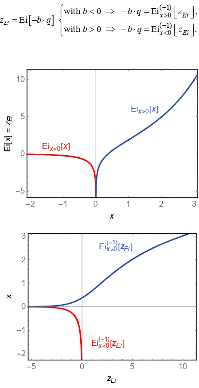
x zEi. There are two reasons for this: First, for negative zEi, Ei( 1) zEi has always two solutions (see Figure 1 bottom), so that Ei( 1) zEi does not represent a true function. One solution corresponds to the case where x is positive in Figure 1 top, and the other where x is negative. To address the problem of calculating the inverse, one has to distinguish between the two branches of the original function (Figure 1 top):
00
Ei for 0,
Ei for 0.
x Ei
x
x x
z
x x
We define the solutions for the inverse in Figure 1 bottom as two distinct (true) functions: x z
Ei
Ei( 1)x0zEi and
Ei
x z Ei( 1)x0zEi. It is clear which case applies in (6): q in Ei
b q
is always positive, and therefore
( 1) 0 ( 1) 0
with 0 Ei ,
Ei
with 0 Ei .
Ei
Ei x
Ei x
b b q z
z b q
b b q z
Figure 1. Top: The exponential integral function
1
2
Ei x lnxx 1! 1 x 2! 2 ... with a singularity at
0
x , where both branches Eix0
x and Eix0
x approach. Upwards, Eix0
x goes to , and Eix0
x to zero.Bottom: For zEi0, the inverse of Ei
x zEi presents two solutions of x. Note that Ei( 1)x0
0, corresponding to
Ei 0 ; Ei( 1)x 0
zEi
0.372507
(when given with six
decimals); Ei( 1)x0
0 ; and Ei( 1)x 0
zEi
approaches quickly
zero for more negative zEi, so that one has to consider sufficient accuracy of the numbers involved in the calculation of zEi.
The second reason, why the inverse function of Ei
x represents a problem, is that there is no formula for calculating it. Only some functions for numerical approximations within certain intervals of x exist (see [9]). One (not very elegant) way to calculate the inverse2 1 0 1 2 3
5 0 5 10
x
E
i
x
zEi
Eix 0x
Eix 0x
5 0 5 10
2 1 0 1 2 3
zEi
x
Eix 0 1
zEi
Eix 0 1
zEi
IAENG International Journal of Applied Mathematics, 48:2, IJAM_48_2_08
indirectly is to repeatedly solve numerically Ei
x zEi: For example, Ei
1.5 is 3.301, when given with three decimals, so that the inverse of the exponential integral function at 3.301 is 1.5 (see Figure 1). To solve, for example,
Ei x 3, one has to search iteratively below 1.5 to find x. In the following, we present a new way of solving this problem. We can express (4) as
1
Ei ln .
! k k
x
x x
k k
(10)The natural logarithm can be represented as an infinite series (page 137 in [6]):
2 1
1
2 1
ln for 0.
2 1 1
k
k
x
x x
k x
(11)Inserting (11) into (10) yields
2 1
1
1 2
Ei .
2 1 1 !
k
k
k
x x
x
k x k k
It turns out that this is equivalent to
Ei
2 atanh 1 0, ln1 x
x x x
x
, (12)
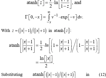
where atanh refers to the inverse hyperbolic tangent function (page 142 in [6]), and to the incomplete gamma function (page 236 in [6]):
1 1
atanh ln , and
2 1
z z
z
1 .
0, exp d
x
x v v v
With z
x 1
x1
in atanh
z :.
1 1 1 1
atanh 1 1
1 1
2 1
ln
2
x x x
ln
x x
x
x
Substituting atanh
x1
x1
in (12), distinguishing between positive and negative x, and simplifying, the following two equations are obtained:
0
0
Ei ln 1 0, ,
Ei 0, .
x
x
x x
x x
These equations provide a mathematical filter to distinguish between the two branches in Ei
x , for x0 and x0, by keeping the branch of interest for given zEi and either positive or negative x, in the domain of real numbers, while moving the other branch into the domain of complex numbers. Not that in the case of x0, ln
1 i isalways in the domain of the complex logarithm, but the imaginary part of Eix0
x at the end becomes zero in thesolution.
Thus, the problem has been converted in the following way: We wish to find x for given zEi, in order to find the value of the inverse functions x z
Ei
Eix( 1)0zEi or
Ei
x z Ei( 1)x0zEi:
ln 1 0, for 0,
0, for 0. Ei
x x
z
x x
(13)
Whereas this still does not provide an explicit formula for
Ei
x z , the advantage of (13) is that there is no ambiguity anymore of two function values for Ei( 1)
x , since the upper and lower branches have been separated (Figure 1 bottom). To find x for given zEi, one has to use a root-finding algorithm (see chapter 9 of [11]).Concerning computation, the numerical evaluation of the incomplete gamma function has been treated in [10], pages 221-224 of [11], and pages 560-567 of [12]. When using Mathematica, the computation of x z
Ei
is summarized in Table 1. The formulas from (13) are given in Table 1, the core code is shown, as well as recommended starting values for the indirect search are provided (see also the section “Supporting Information” at the end of the article).TABLE 1. SUMMARY FOR CALCULATING NUMERICALLY THE INVERSE OF THE EXPONENTIAL INTEGRAL FUNCTION zEiEi
x
Ei
x z ( 1)
0
=Eix zEi =Ei( 1)x0zEi
Formula
Given zEi, solve zEi
ln 1 0, x
numerically for x in the domain of real numbers
Given zEi, with
0
Ei
z , solve
0,
Ei
z x numerically for x in the domain of real numbers (zEi0 does not exist in this branch)
Mathematica
code
Re[ FindRoot[ zEi = =
Log[1] Gamma[0,
x], {x, zStart}, WorkingPrecision
>30, MaxIterations
>1000]
Re[ FindRoot[ zEi = =
Gamma[0, x], {x, zStart},
WorkingPrecision
>30, MaxIterations
>1000]
Recommended values for zStart
for 1: 10 Ei, and Ei
z z
for zEi1: lnzEi
for 0.5: exp , and
Ei
Ei
z z
for 0.5 0:
ln
Ei
Ei
z z
IAENG International Journal of Applied Mathematics, 48:2, IJAM_48_2_08
[image:4.612.71.298.212.361.2] [image:4.612.69.293.422.587.2]There is one closely related, as well as another, completely different approach to find numerically the inverse of the exponential integral function. First, one can use (5a) with ln
x for Eix0
x and ln
x for
0Eix x , instead of lnx. The accuracy is controlled with the remainder of (5b). The second approach, given in the supporting information, consists of a segment-wise numerical simulation of the two branches of the function in Figure 1 bottom, with high-degree polynomials (e.g., 31 coefficients) and a high number of calculated data points (e.g., 10,000) in each of several segments.
IV. THE FINAL FORMULAS OF THE GENERALIZED
EXPONENTIAL FUNCTION
Employing the inverse of Ei
x , (6) can now be re-arranged to calculate q t
, rather than t q
. With ttC and qC 0, we define the generalized exponential function as:
( 1) 0
( 1) 0
exp 1
Ei for 0,
+Ei
exp exp for 0,
exp 1
Ei for 0,
+Ei
C C
C C
C C
x
x
t t a
b
b b q
q t q t t a b
t t a
b
b b q
(14)
where b0 represents sigmoid growth, b0 exponential growth, and b0 explosive growth, and where for b0 the restriction
t t C
exp a
+Ei
b qC
0 applies. Rearranging this restriction leads toEi for 0
exp
C C
b q
t t b
a
. (15)
The restriction in (15) represents an upper bound for t, and reflects the fact that for explosive growth with given coefficients, there is a maximum time t that can be reached for given parameters a, b, qC, and tC, no matter how large
q is.
We call (14) “generalized exponential function”. The term has rarely been used before for other functions. In unrelated form, the term “generalized (q-)exponential function” is used in [13] (page 2923) to refer to
lim 1'
'
1 'q.q q q
e x q x
In [14] (page 574), the term
“generalized exponential growth model” is employed for
exp
1f t a b t .
Note that in computations with (14) one can also use the formulas for b0 arbitrarily close to b0, instead of using the one for b0. One can show this with (6), the formulas that form the basis for (14). Using (4) and b0, the formulas convert into each other:
1 2
Ei 0 Ei 0
0 0
ln ln ...
1! 1 2! 2
ln ln .
C
C C
C
C
q q
q q q q
q q
q q
For sigmoid growth (b0) in (14), and t , q t
will not converge to a maximum quantity. Using (2), one can see that q t
q t
exp[a b q t
], which for increasing
0q t remains always positive.
Equation (14) with b0 represents the formula for calculating relative growth from a smaller qC to a larger
ln
ln
C
C
q t q q tt , suggested already as the “correct” formula by Sir Ronald Fisher in 1921 [15]. It reflects exponential growth. Whereas this formula is relatively well-known by field biologists, (14) with b0 for sigmoid growth and for explosive growth, as the more general cases, are new.
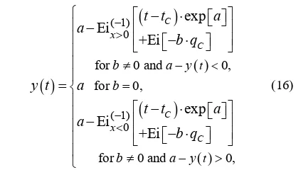
For calculating the logarithmic relative growth at any time, q in (9) is substituted by q t
from (14):
( 1) 0
( 1) 0
for 0 and 0,
for 0,
for 0 and 0,
exp Ei
+Ei
exp Ei
+Ei
C C
C C
x
x
t
t
b a y
b
b a y
t t a
a
b q
y t a
t t a
a
b q
(16)
where for b0 the restriction of (15) applies. With the left-hand side y t
involved in the condition to choose among options for b0, this formula is only practical if one knows that ay t
will be positive or negative. Otherwise, if one does not want to calculate t y
instead of y t
, the alternative is to employ (9), where q t
has to be calculated first with (14).Furthermore, the instantaneous increment as a function of time is
exp for 0,
exp exp for 0,
C C
t t
q a b q b
q t
q a t t a b
(17)
where in the case of b0, q t
has to be calculated first with (14). Introducing (14) for q t
in (17) would not lead to simplification, but would involve twice the inverse of
Ei x , causing in turn complicated conditions if
( 1) 0
Eix zEi or Ei( 1)x0zEi applies. For b0, the formula is derived from (2). For b0, the formula is derived from (14) by taking the derivative.
IAENG International Journal of Applied Mathematics, 48:2, IJAM_48_2_08
[image:5.612.327.535.318.438.2]V. DETERMINATION OF THE FUNCTION PARAMETERS FROM THREE DATA POINTS
The generalized exponential function of (14) with b0 is a three-parameter model, whose parameters a, b, and qC (at tC) or tC (at qC) are thus determined exactly by three points q1 at t1, q2 at t2, and q3 at t3, with t1t2t3 and q1q2q3 or q1q2q3. Given such three data points, any one can represent qC at tC. To determine b, one has to solve the following relationship numerically and indirectly (in Mathematica with the FindRoot function, with
1
being generally a recommended starting value):
3 1 3 1
2 1
2 1
Ei Ei
Ei Ei
b q b q t t
t t
b q b q
. (18)
The formula is derived by transforming the equation of (7) for b0 with q1 at t1 being the calibrating point qC at tC, resulting in exp
a
Ei
b q
Ei b q1
t
q t1
. By substituting q at t
q with q2 at t2 on the one hand, and with q3 at t3 on the other, one obtains two equations for exp
a , which are set equal. Having determined b, one calculates3 1
3 1
Ei Ei
ln b q b q .
a
t t
Since the generalized exponential function represents a continuous spectrum of growth functions from sigmoid to explosive, one expects to always find a solution for b in (18), and subsequently for a. Note that the three points may lie on a straight line, but that the resulting function will represent nevertheless in that case a sigmoid curve among the points.
An alternative method to determine a and b for b0 is to use nonlinear regression with (6), which (at least in Mathematica) works well. The regression equation is
1 Ei b q Ei b q1 exp a
tt . With three data points of t
q , the resulting coefficient of determination has to be 1. The regression can also be used for more than three data points, in which case it becomes a true regression analysis, with (generally) variance of the residuals and2 1
R . In that case, one can also let the regression determine either
q
C ort
C. Note, however, that the residuals present time, rather than quantity.VI. INFLECTION POINT IN NON-EXPONENTIAL GROWTH
An inflection point refers to the point on a growth curve, where the curve switches from being left-winged (locally convex) to being right-winged (locally concave), or vice versa (circles in Figure 2). Knowing and analyzing a
formula for the inflection point is of interest for several reasons:
(i) The inflection point characterizes the shape and scale of a growth curve. In a nonlinear growth curve model, there are few points on the curve that can be used to compare different curves of a given function: In the case of the generalized exponential function, there is one calibrating point (qC at tC), as well as for b0 the inflection point (qIP at tIP).
(ii) The formula for calculating the location of the inflection point reveals important information about the dependence of the growth curve’s shape, location, and scale on the different parameters: How does changing the function’s parameters affect the inflection point, and consequently the whole growth curve?
(iii) It can also be of interest to develop a growth curve around a known inflection point, i.e., to derive the growth function’s parameters with a known (fixed) inflection point.
The inflection point quantity (qIP) is derived by taking the second derivative of (6) for b0 with respect to q:
2 2
2. d
t
dq 1 b q exp a b q q (19) Setting this expression equal to zero, and solving for q, yields:qIP 1b, (20) which is positive only for b0. This relation reveals a surprisingly simple interpretation of b as the negative inverse of the inflection point quantity. For b0, i.e., explosive growth, qIP would be negative, which however has no real-world interpretation, and thus will not be considered further.
Inserting (20) into (6) for b0 results in the corresponding inflection point time (tIP):
Ei 1 Ei
for 0, exp
C
IP C
b q
t t b
a
(21)
where Ei 1
1.89512, when given with five decimals. Furthermore, as a necessary condition, one has to show that there is a change of sign of the second-derivative at the inflection point (page 231 in [16]). With q0, the second factor exp
a b q
q2 in (19) will always be positive. Therefore, if the second derivative will be positive or negative depends only on the first factor
1 b q
in (19). For b0,
1 b q
0 implies q 1b, whereas
1 b q
0 implies q 1b. For b0,
1 b q
0 implies q 1b, whereas
1 b q
0 implies q 1 .bIAENG International Journal of Applied Mathematics, 48:2, IJAM_48_2_08
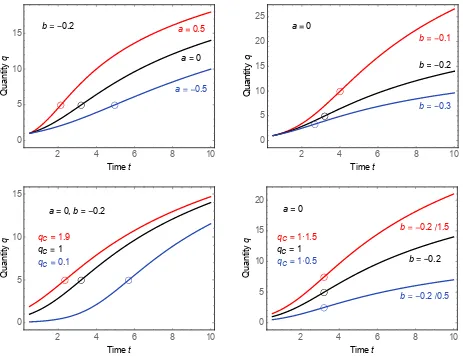
Figure 2. Variations of sigmoid growth curves (b0), when changing symmetrically the growth rate parameter a, the shape and scaling parameter b, or the quantity qC of the calibrating point at tC0.5 in (14) with b0. Top left: Change of a0 (initial relative growth is 100%) by 0.5. Top right: Change of b 0.2 (qIP5) by 0.1. The new inflection point quantity is qIP
1 b b
, and the new inflection point time has to be calculated with (21). Bottom left: Change of qC1 by 0.9 without changing b, i.e., the inflection point quantity (circles) moves horizontally. Bottom right: Changing qC and b according to (23) changes the growth curve’s scaling, and moves the inflection point quantity vertically. Note that relative growth remains the same for all three curves at any time in this graph, since
ya b f q f a b q.
Consequently, there is always a change of sign at qIP. Since the second derivative switches from negative to positive at the inflection point with increasing q, the formula also proves that the function switches always from right-winged to left-winged for b0. Recall, however, that (6) is the formula for t
q . In the case of q
t in (14), the curve’s shape changes to its mirror image, resulting for0
b always in a growth curve that switches inversely from being left-winged to being right-winged.
Depending on tC, b, and qC, the inflection point time IP
t can be positive or negative; a negative inflection point time for b0 means that tIPtC, i.e., only the
right-winged (concave) part of the growth curve appears for positive time.
VII. THE RELATIONSHIP AMONG THE PARAMETERS a,b,
AND qC AT tC
In the generalized exponential function, the three parameters a, b, and qC at tC have straight-forward interpretations: Whereas qC at tC calibrates the position of the growth curve segment, a is the initial logarithmic relative growth, i.e., the intercept at q0 (see Figure 3 bottom). It serves as a standardized growth rate parameter (see Figure 1 in [8]).
2 4 6 8 10
0 5 10 15
Timet
Q
u
a
n
ti
ty
q
b 0.2
a 0.5
a 0
a 0.5
2 4 6 8 10
0 5 10 15 20 25
Timet
Q
u
a
n
ti
ty
q
a 0
b 0.3
b 0.2
b 0.1
2 4 6 8 10
0 5 10 15
Timet
Q
u
an
ti
ty
q
a 0,b 0.2
qC 0.1
qC 1
qC 1.9
2 4 6 8 10
0 5 10 15 20
Timet
Q
u
an
ti
ty
q
a 0
b 0.2 0.5
b 0.2
b 0.2 1.5
qC 1 0.5
qC 1
qC 1 1.5
IAENG International Journal of Applied Mathematics, 48:2, IJAM_48_2_08
On the other hand, b is a shape parameter in terms of its sign, as well as a scaling parameter in terms of its magnitude.
Different combinations of parameter values between a and b cause different curvatures. Note that the second derivatives of (6) for b0, as measures of the curvature, depend on both a and b:
d22 Ei Ei ,
exp d
C
b q b q
a a
t
(22a)
2
2 2
.
d 1
exp d
1 exp 1 exp
C
C C
a b q q
b b
b q b q b q b q
t
(22b)
For example, the more negative a in (22a), the larger is the curvature. Extreme curvatures are associated with extreme parameter values of a and b.
Figure 2 shows different combinations among the three parameters a, b, and qC in the case of sigmoid curves (b0). Changing tC is not shown in Figure 2, because it only moves the whole curve to the left or right, as can be seen from (6). The inflection points are indicated with circles in Figure 2. In Figure 2 top left, the parameter a is varied around a0 (i.e., initial relative growth is 100%). One sees that a symmetrical change of a (here 0.5) leads to symmetrical growth curves around the original curve, with constant qIP but different inflection point times tIP. This is not the case for a symmetrical change of b (here
0.1
), which results in asymmetrical curves around the original growth curve (Figure 2 top right). In Figure 2 bottom left, qC is moved up and down by the same amount (here 0.9 ). The qIP, however, are kept constant, which causes asymmetrical shapes of the resulting growth curves around the original one. Changing both the quantities of qC and qIP (via b) together by the same proportion results in a change of scale, shown in Figure 2 bottom right and explained next.
In addition to b determining if the growth curve is sigmoid, exponential, or explosive, the variables b and qC are scaling q t
. In (14) with b0, one can multiply qC by some factor, and divide b by the same factor (say f ), to model a growth curve of qf
t f q
t :
( 1)
exp
Ei .
+Ei C
f
C
t t a
f
q t b
b q f
f
(23)
The shape of the curve remains the same, with the new inflection point quantity f q IP, but unchanged inflection point time. The factor f does neither affect the initial logarithmic growth rate a, nor y in (9) or (16).
VIII. NEGATIVE GROWTH WITH THE GENERALIZED EXPONENTIAL FUNCTION
According to the standard exponential function, growth can be positive or negative. To describe negative growth with the generalized exponential function, presented in (14), one has to replace t t C with tCt. We add the subindex NG for negative growth, so that (14) changes to
( 1) 0
( 1) 0
exp 1
Ei for 0,
+Ei
exp exp for 0,
exp 1
Ei for 0,
+Ei
C
C
NG C C
C
C
x
x
t t a
b
b b q
q t q t t a b
t t a
b
b b q
(24)
where b0 represents negative sigmoid growth, b0 negative exponential growth, and b0 negative explosive growth. The restrictions in (8), when b0, convert to
for , and for .
NG C C NG C C
q q tt q q tt
Furthermore, (15) changes for negative growth:
for 0 and negative growth.
Ei
exp
C
C b
b q t t
a
Finally, (21) converts to
for 0 & negative growth.
Ei 1 Ei
exp
C
IP C b
b q
t t
a
For negative growth, one also substitutes t t C with tCt in (7) for calculating a, in (16) for calculating y t
, and in (17) for calculating q t
.IX. GENERALIZED VERSUS STANDARD EXPONENTIAL
GROWTH
To show how the formulas work, and how the generalized exponential function compares with the standard exponential function, some sample growth curves are shown in Figures 3 and 4. To get a sigmoid growth curve with inflection point tIP7, qIP 5, and calibrating point
2 C
t , qC 1, according to (20) one uses b 0.2. To calculate the corresponding a, one has to transform (21):
Ei 1 Ei
ln C for 0.
IP C
b q
a b
t t
The restrictions from (8) become qIPqC for ttC, and
IP C
q q for ttC. For negative growth, one has to substitute tCtIP for tIPtC, with qIPqC for ttC, and qIPqC for ttC. Here, one gets a 0.610.
IAENG International Journal of Applied Mathematics, 48:2, IJAM_48_2_08
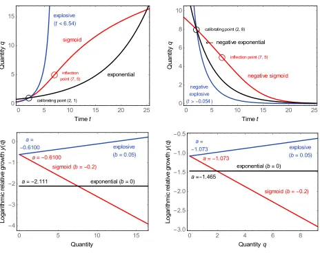
[image:8.612.319.540.149.242.2]Figure 3. Sigmoid growth (b0), exponential growth (b0), and explosive growth (b0), positive (left) and negative (right). Top: Quantity q as a function of time, as calculated with (14) for positive growth (left), and with t tC substituted by tCt in (24) for negative growth (right). Whereas the parameter b determines the shape and scale of the function, a determines the relative growth rate, and the calibrating point qC
tC the position of the growth curve in the upper graphs. Bottom: The underlying linear relationship of logarithmicrelative growth y as a function of q, as calculated with (9) for positive or negative growth, which cannot be distinguished in these two graphs. Whereas b is the slope in this functional relationship, a is the intercept at a quantity of zero.
Using (14) with b0, Figure 3 top left shows the resulting sigmoid growth curve. Going through qC 1 at
2 C
t , the curve reaches q16.2 at t25. Employing (7) for b0, one can calculate the logarithmic relative growth rate for an exponential growth curve that also goes through q1 at t2 and q16.2 at t25, which results in a 2.11. The corresponding growth curve, calculated with (14), is shown in Figure 3 top left.
Negative growth is shown in Figure 3 top right, employing (24) for negative sigmoid growth, negative exponential growth, and negative explosive growth, with the same parameters of b as for positive growth, but choosing
IP C
q q (and calculating the corresponding parameters for a).
Figure 3 bottom shows the corresponding linear relationships between q t
and logarithmic relative growth, as given in (2). In those graphs, a is the intercept and b is the slope of the lines (qC at tC does not appear in this mathematical relationship).Figure 4 shows two more functional relationships for the growth curves from Figure 3 top. For sigmoid growth, there appears a maximum of the instantaneous increment with time. This maximum is at the inflection point time.First, the relationship between tIP and qIP is given bysubstituting
b in (21) with b 1qIP from (20), and rearranging:
Ei 1 exp Ei
exp
C
IP C
IP q
t t a
q a
. (25)
0 5 10 15 20 25
0 5 10 15
Timet
Q
u
a
n
ti
ty
q
calibrating point 2, 1
inflection point 7, 5 sigmoid explosive
t 6.54
exponential
0 5 10 15 20 25
0 2 4 6 8 10
Timet
Q
u
a
n
ti
ty
q
calibrating point 2, 8
inflection point 7, 5
negative sigmoid
negative explosive
t 0.054
negative exponential
0 5 10 15
4 3 2 1 0
Quantity
L
o
g
a
ri
th
m
ic
re
la
ti
v
e
g
ro
w
th
y
q
sigmoid b 0.2 a 0.6100
a
0.6100
a 2.111
explosive
b 0.05
exponential b 0
0 2 4 6 8
3.0 2.5 2.0 1.5 1.0 0.5
Quantityq
L
o
g
a
ri
th
m
ic
re
la
ti
v
e
g
ro
w
th
y
q
sigmoid b 0.2 a
1.073
a 1.073
a 1.465
explosive
b 0.05
exponential b 0
IAENG International Journal of Applied Mathematics, 48:2, IJAM_48_2_08
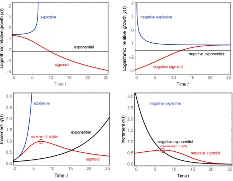
Figure 4. Two additional functional relationships for the positive (left) and negative (right) growth curves of Figure 3 top. Top: Logarithmic relative growth y as a function of time, calculated with (16) for positive growth, and with t tC substituted by tCt for negative growth.
Bottom: Instantaneous increment q t
as a function of time, calculated with (17) for positive growth, and with t tC substituted by tCt for negative growth. For sigmoid growth (b0), there is a maximum at the inflection point time, calculated with (26).Next, to calculate the maximum instantaneous increment, one substitutes
t
in (17) for b0, with tIP from (25), which yields
max 1 exp a 1 for b 0. bq t
(26)The formula applies for both positive and negative growth.
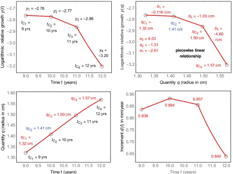
X. CONVERSION OF A SEGMENTED CURVE OF y t
INTO AGROWTH CURVE OF q t
Assume that there are two known points of logarithmic relative growth, yi at ti and yi1 at ti1, where the integer subindex i serves to index and distinguish the points (a
larger i refers to a later time point). Then one can find the corresponding ai and bi for the generalized exponential function that goes from the first to the second point. The procedure will be useful, for example, for statistical applications. There may be more than two subsequent points
i
y at ti, and one wants to use (16) to get a continuous function through all points, employing splines (Figure 5 top left). This segmented function can then be converted into a growth curve of quantity as a function of time (Figure 5 bottom left). The method works only for segments with
0,
b but b can be arbitrarily close to 0.
Transforming (16) for b0, one gets two equations for a single segment of the generalized exponential function, where the subindex i refers to the function segment (spline) in between time points ti and ti1:
0 5 10 15 20 25
4 3 2 1 0 1 2
Timet
L
o
g
a
ri
th
m
ic
re
la
ti
v
e
g
ro
w
th
y
t
sigmoid explosive
exponential
0 5 10 15 20 25
3 2 1 0 1 2
Timet
L
o
g
a
rit
h
m
ic
re
la
ti
v
e
g
ro
w
th
y
t
negative sigmoid negative explosive
negative exponential
0 5 10 15 20 25
0.0 0.5 1.0 1.5 2.0 2.5 3.0
Time t
In
c
re
m
e
n
t
q
'
t
sigmoid maximum 7, 0.999
explosive
exponential
0 5 10 15 20 25
0.0 0.5 1.0 1.5 2.0 2.5 3.0
Timet
In
c
re
m
e
n
t
q
'
t
negative sigmoid maximum 7, 0.629
negative explosive
negative exponential
IAENG International Journal of Applied Mathematics, 48:2, IJAM_48_2_08
1 1
Ei exp +Ei ,
Ei exp +Ei .
C C
C C
i i
i i
i i i i i
i i i i i
a y t t a b q
a y t t a b q
With C
i i
t t , the first equation simplifies to ,
Ci
i i i
a y b q which corresponds to (9). Substituting ai in the second equation with C
i i i
y b q yields
1
1
Ei Ei
exp 0 for 0.
i
C C
C
i
i
i i i i
i i i i
i
y y b q b q
t t y b q b
(27)
The variables bi and C i
q occur always together as C i i
b q
in (27). With (20), this term converts to C IP i i
q q within a given segment. With the definition of the ratio
i i Ci Ci IPi
r b q q q , and rearranging for more robust root-finding, (27) becomes
Ei 1 Ei
1
0,exp
i i i i
i i i i
y y r r
t t y r
(28)
with yi yi1 (which is equivalent to b0). With (28), one can indirectly find the ri, given yi, yi1, and ti 1 ti
, with a root-finding method (in Mathematica the function “FindRoot”; a recommended starting value is 1). In accordance with (9), ai is calculated for the segment between the two points subsequently as
ai yiri, (29) where the last yi (
t n
y ) is not being used (there are nt1 data of each ai and ri, but nt data of yi).
Next, for calculating the growth curve of q t
, the numerical values of bi and Ci
q are needed separately, rather than combined in ri. Assuming that there are nt points yi at ti, one has to determine nt1 segments as continuous functions that connect the points non-linearly, according to (16). With the nt points of logarithmic relative growth y ti
i , the nt 1 parameters of ri and ai, and a single known calibrating point Ci
q , one can find bi and C i q of all segments simultaneously: Using (7) for b0, one obtains
1
1 1 1 1 1 1
exp Ei Ei
1
Ei Ei .
C C
C C
i i
i i
i i i
i i
i
i i
i i
i
a b q b q
t t
b
b q b q
t t b
Defining the coefficient ci b bi i1, and as before Ci
i i
r b q and
1
1 1 Ci
i i
r b q
, one gets
1
1 1
exp i Ei i i Ei i .
i i
a c r r
t t
Now only the ci are still unknown. Rearranging further yields
1 1
Eic ri i ti ti expai Ei ri .
The inverse exponential integral function has to be applied to the left-hand side: If c rii10, then ( 1)
0 Eix zEi
applies, and if c rii10, then ( 1)
0Eix zEi applies. Given that
1
1 Ci
i i i
c r b q
, and
1 0 Ci q
, the sign of bi
determines which inverse function has to be used. Since Ci
i i
r b q :
( 1) 1 ( 1) 1 0 00 0 0 Ei ,
0 0 0 Ei .
Ei Ei
i i i i x
i i i i x
r b c r z
r b c r z
Consequently, the formula for calculating ci equals
( 1) 0 1 1 ( 1) 0 1 1Ei exp Ei
for 0,
Ei exp Ei
for 0. x
i x
i i i i
i i
i i i i
i i
t t a r
r r
c
t t a r
r r (30)
The case C