Shengju Sang
FF Abstract—This paper explores the influences of reference price effect and fairness concerns on the pricing policies and green strategies in a two-echelon green supply chain with one manufacturer and one retailer. Three game theory models with Manufacturer-Stackelberg (MS) game, Retailer-Stackelberg (RS) game and Vertical-Nash (VN) game are developed, and their optimal solutions are also derived. Finally, the results of the proposed game models are analyzed via a numerical example. The results show that the wholesale price, the greening level, and the retail price are lower in the scenario with the reference price effect and the fairness concern than without. The retailer can benefit in the three games, while the manufacturer can suffer in the MS and RS games with consideration of the reference price effect and the fairness concerns.
Index Terms—green supply chain, reference price effect,
fairness concern, game theory
I. 0BINTRODUCTION
ITH economic globalization and environmental resources issues becoming increasingly prominent, the green supply chain is becoming a hot topic and capturing keen scientific attention. The application of green supply chain management can improve the environmental and economic performance of supply chain members, as well as enable members to obtain competitive advantage, which encourages supply chain to be continually sustainable.
As green policies have received increasing attention, there is wide research on the appropriated operation decisions under green supply chain. Some researchers are interested in studying the problems of the pricing and coordination strategies in green supply chains. For example, Ghosh and Shah [1] developed game theoretic models in a green supply chain and studied the impact of channel structures on the greening levels, prices and profits. Xie et al. [2] considered the selection of cleaner products in a green supply chain, where the manufacturer and the retailer faced financial risk. Xie et al. also [3] investigated the selection of cleaner products with the consideration of the tradeoff between risk and the return of players in a green supply chain. Xie [4] analyzed the impact of the threshold
Manuscript received May 01, 2018; revised September 15, 2018. This work was supported by the Humanity and Social Science Youth Foundation of the Ministry of Education of China (NO.17YJC630116), the Shandong Provincial Soft Science Foundation, China (No. 2018 RKB01060), and the Project of Shandong Provincial Higher Educational Humanity and Social Science Research Program (No. J18RA050).
Shengju Sang is with the School of Business, Heze University, Heze, 274015, China (phone: +86 15853063720; e-mail: sangshengju@163. com).
value of energy saving levels on energy saving levels and the price with an integrated structure and a decentralized setting in a green supply chain. Liu and Yi [5] studied the pricing policies of green supply chain considering targeted advertising and product green degree in the Big Data environment. Swami and Shah [6] proposed a two part tariff contract to coordinate the green channel with a manufacturer and a retailer. Zhang and Liu [7] studied the coordination mechanism by using a revenue sharing mechanism, Shapley value method coordination mechanism and asymmetric Nash negotiation mechanism in a three stage green supply chain. Zhang et al. [8] also investigated the pricing and coordination strategies of green supply chain under hybrid production mode. Ghosh and Shah [9] explored the supply chain coordination issues by two cost sharing contracts, one in which the retailer offered a cost sharing contract and the other in which the retailer and the manufacturer bargained on the cost sharing contract. Huang et al. [10] studied the green supply chain coordination with multiple suppliers, a single manufacturer and multiple retailers by a game-theoretic model. Basiri and Heydari [11] investigated the green channel coordination issue in a two-stage supply chain with a non-green traditional product and a new substitutable green product. Song and Gao [12] developed two green supply chain game models under the revenue sharing contract and showed this contract could improve the greening level of the products. Some research has also begun to emerge in the area of the competition of green supply chain. Sheu [13], Sheu and Chen [14] analyzed the impact of governmental intervention on competing green supply chains. Li et al. [15] studied the optimal pricing and greening strategies in a competitive dual-channel supply chain. Chen et al. [16] studied the pricing and greening level strategies in a duopoly green supply chain with a green manufacturer, a traditional manufacturer and a common retailer under vertical and horizontal competition. Hafezalkotob [17] considered price and energy saving competition and cooperation models between two green supply chains under government financial intervention. Zhu and He [18] investigated the green product design problems in green supply chains under competition including a horizontal retailer competition case and six cases of competing supply chains. Recently, Yang and Xiao [19] studied the pricing and greening level decisions in a green supply chain with governmental interventions under fuzzy uncertainties. Sang [20] developed three different decentralized decision models of green supply chain, in which the demand and cost were fuzzy.
All studies mentioned above discussed the green supply chain issues assumed that the supply chain members were
Optimal Policies in a Green Supply Chain with
Reference Price Effect and Fairness Concern
W
IAENG International Journal of Applied Mathematics, 48:4, IJAM_48_4_15
rational-economic men, who always tried to maximize their own profits. However, abundant evidence shows that supply chain members not only care about their own profits, but also the profit difference between the two sides, meaning they concern about fairness. Cui et al. [21] investigated how fairness concerns affected channel coordination in a supply chain. Caliskan-Demirag et al. [22] studied the supply chain coordination problem under fairness concerns with nonlinear demand functions. Yang et al. [23] studied the cooperative advertising problem in a distribution channel with a manufacturer and a retailer when the retailer had fairness concerns. Du et al. [24] studied a newsvendor problem in a dyadic supply chain in which both the supplier and the retailer had the preference of status-seeking with fairness concerns. Recently, Nie and Du [25] investigated quantity discount contracts with two fairness concerned retailers in a dyadic supply chain. Sang [26] studied the pricing and retail service level decisions between one manufacturer and one retailer when the manufacturer had fairness reference.
In addition, some previous empirical studies have demonstrated that reference price significantly affects the market demand. Reference price, which is the cognitive price that consumers form based on historical prices of the product, plays a key role in the purchase decisions of consumers. Zhang et al. [27] studied the equilibrium pricing strategies between the retailer and the manufacturer with reference effects in a competitive supply chain. Lin [28] studied the price promotion problem with the reference price effects of consumers in a supply chain. Xu and Liu [29] studied the optimal decisions of the manufacturer, the retailer and the third party in a closed loop supply chain with reference price effect.
However, very few studies have addressed the issues of reference price effect and fairness concerns in a green supply chain. Therefore, it is important to study the pricing and greening level decisions when the consumer has reference price and the supply chain members have fairness concerns. In this paper, we discuss the pricing and greening level decisions with a manufacturer and a retailer, in which the consumer has reference price and the retailer has fairness concerns. We mainly discuss the conditions where the manufacturer and the retailer pursue three different power structures: pursuing the Manufacturer-Stackelberg game, playing the Retailer-Stackelberg game and acting in the Vertical- Nash game.
The rest of paper is organized as follows. Section II briefly describes the problem and the notations in our models. Section III develops three non-cooperative games between the manufacturer and the retailer when the retailer has fairness concerns. A numerical example is provided to illustrate the results of the proposed models in Section IV. Finally, Section V summarizes the work done in this paper and further research areas.
II. 1BPROBLEM DESCRIPTIONS
This paper considers a two-echelon green supply chain consisting of a manufacturer selling his green product to a retailer, who in turn retails it to the consumer. We assume the manufacturer produces only one green product and the retailer sells only single product.
Following Ghosh and Shah [1], Xu and Liu [29], we model the demand faced by the manufacturer and the retailer as a linear function of the retail pricep, the greening levelθand the reference price of the consumerr, which is given by
(
)
q= −α βp+γθ λ− p r− (1) where the parameterαrepresents the market potential, the parameterβ represents the sensitivity of demand to price changes, the parameterγrepresents the demand expansion effectiveness coefficient of the greening level by the manufacturer and the parameterλrepresents the reference price coefficient.
Further, letwdenote the wholesale price per unit charged to the retailer by the manufacturer, cthe manufacturer’s cost of producing its green product andmthe retailer’s profit margin on the green product. As the retail price can be considered as the total of the profit margin and wholesale price, we consider retail price as p= +m w . Then the demand for the product can be rewritten as
(
)
(
)
q= −α β m w+ +γθ λ− ⎡⎣ m w+ −r⎤⎦ (2) It is assumed that the greening level modeled here does not affect the manufacturer’s marginal cost. Further, the cost of achieving green innovation requires fixed investment, which is a quadratic function of the level of greening levelθ. It is given by1 2
2ηθ , where the parameterηis the investment coefficient.
According to the problem descriptions, the profits of the manufacturer and the retailer can be expressed as, respectively
(
)
{
(
)
(
)
}
1 22
M w c α β m w γθ λ m w r ηθ
Π = − − + + − ⎡⎣ + − ⎤⎦ − (3)
(
)
(
)
{
}
R m α β m w γθ λ m w r
Π = − + + − ⎡⎣ + − ⎤⎦ (4) We assume that the manufacturer is fairness neural and his utilityUMequals his profitΠM, that is
(
)
{
(
)
(
)
}
1 22
M M
U = Π = −w c α β− m w+ + −γθ λ⎡⎣m w r+ − ⎤⎦ − ηθ (5) The retailer has fairness concern and her utilityUM is
given as follows
(
)
R R M R
U = Π −δ Π − Π
(
1 δ)
m{
α β(
m w)
γθ λ(
m w r)
}
= + − + + − ⎡⎣ + − ⎤⎦
(
)
{
(
)
(
)
}
22
w c m w m w r δ
δ α β γθ λ ηθ
− − − + + − ⎡⎣ + − ⎤⎦ + (6)
whereδ is the retailer’s fairness concern parameter and
[ ]
0,1δ∈ . Whenδ =0, it means the retailer is fairness neutral, and he does not concern fairness. The greater it is, the more the retailer is concerned about the fairness of the distribution.
III. 2BMODELS ANALYSIS
In this section, we analyze the manufacturer and the retailer how to set their optimal policies when they pursue different power structures in a green supply chain. The manufacturer determines the wholesale price and the
IAENG International Journal of Applied Mathematics, 48:4, IJAM_48_4_15
greening level, and the retailer decides the profit margin. We mainly discuss the conditions where they pursue three non-cooperative games: the manufacturer leads the supply chain, the retailer leads the supply chain, and they have the same power.
A. Manufacturer-Stackelberg game
Under the MS (Manufacturer-Stackelberg) game, the manufacturer holds more bargaining power than the retailer. Thus, the manufacturer acts as the Stackelberg leader and the retailer acts as the Stackelberg follower. That is, firstly, the manufacturer sets the wholesale price w and the greening levelθby using the retailer’s reaction function. Then, the retailer sets the profit marginmso as to maximize his utility.
We first obtain the optimal reaction function of the retailer. Proposition 1 gives the result.
Proposition 1. Under the MS game, the optimal reaction function *
(
)
,
m wθ of the retailer can be given by considering the wholesale price and the greening level made earlier by the manufacturer
(
)
(
(
)
)
(
(
)
)
* ,
2 2 1
r w w c
m wθ α λ β λ γθ δ
β λ δ
+ − + + −
= +
+ + (7)
Proof. Referring to (6), we can get the first order derivative of URtomas follows
(
)(
)
(
)
(
)
d
2 1 1
d
R
U
m w
m = − +δ β λ+ − β λ+ + +δ γθ
(
1 δ α λ)(
r) (
δ β λ)
c+ + + − + (8) Then, the second order derivative ofURtomcan be shown as
(
)(
)
2
2
d
2 1 d
R U
m = − +δ β λ+
Note that the second order derivative of UR tom is
negative definite, since β >0 , λ>0 and 0≤ ≤δ 1 . Consequently, URis strictly concave inm.
Setting (8) to zero, the first order condition can be shown as
(
)(
)
(
)
(
)
2 1 δ β λ m β λ w 1 δ γθ
− + + − + + +
(
1 δ α λ)(
r) (
δ β λ)
c 0+ + + − + = (9) Solving (9), we obtain
( )
(
(
)
)
(
(
)
)
*
2 2 1
r w w c
m w α λ β λ γθ δ
β λ δ
+ − + + −
= +
+ +
The proof of Proposition 1 is completed.
After knowing the retailer’s reaction function, the manufacturer would use it to maximize his utility by choosing the wholesale price and the greening level.
Proposition 2. Under the MS game, if4
(
β λ η γ+)
> 2, then the optimal policies of the manufacturer and the retailer are
(
)
(
)
(
)(
) (
)
*
2
2 1
4 1 2 1
r c
w δ η α λ β λ c
δ β λ η δ γ + ⎡⎣ + − + ⎤⎦
= +
+ + − + (10)
(
)
(
)
(
)(
) (
)
*
2
1
4 1 2 1
r c
δ γ α λ β λ θ
δ β λ η δ γ + ⎡⎣ + − + ⎤⎦ =
+ + − + (11)
(
)
(
)
(
)(
) (
)
*
2
1 5
4 1 2 1
r c
m δ η α λ β λ
δ β λ η δ γ + ⎡⎣ + − + ⎤⎦ =
+ + − + (12)
Proof. Substituting *
(
)
,
m wθ in (7) into (5), we can get the utility of the manufacturerUMas follows
(
)
(
)
(
)(
)
21 1
2 1 2
M
w c
U w c α λr β λ w γθ δ β λ ηθ
δ
+ −
⎡ ⎤
= − ⎢ + − + + − + ⎥−
⎣ ⎦ (13)
From (13), we can get the first order derivatives ofUMtowandθas follows
(
)
(
)(
)
1 2 1 1 1 3
1 2 2 2 1
M U
w c
w
δ β λ γθ α δ β λ
δ δ
∂ = − + + + + + + +
∂ + + (14)
1 1
2 2
M
U
w c
ηθ γ γ θ
∂
= − + −
∂ (15) Then, the second order derivatives ofUMtowandθcan be shown as
(
)
2
2
1 2 1
M U
w δδ β λ
∂ +
= − +
+
∂ ,
2
1 2
M U w θ γ
∂ =
∂ ∂ ,
2
2 M
U η
θ
∂
= −
∂ ,
2
1 2
M U
w γ
θ
∂ =
∂ ∂ .
Thus, the Hessian matrix can be obtained as
(
)
2 2
2
2 2
2
1 2 1
1 2
1 2
M M
M M
U U
w w H
U U
w
δ β λ γ
θ δ
γ η
θ θ
∂ ∂ +
− +
∂ ∂
∂ +
= =
∂ ∂ −
∂ ∂ ∂
Note that the Hessian matrix is negative definite, since4
(
β λ η γ+)
> 2 and0≤ ≤δ 1. Consequently, UM isstrictly jointly concave inwandθ.
Setting (14) and (15) to zero, the first order conditions can be shown as
(
)
(
) (
)
1 2 1 1 1 3
0
1 w 2 2 2 1 c
δ β λ γθ α δ β λ
δ δ
+ +
− + + + + + =
+ + (16)
1 1
0 2 w 2 c ηθ γ γ
− + − = (17) Solving (16) and (17), we obtain
(
)
(
)
(
)(
) (
)
*
2
2 1
4 1 2 1
r c
w δ η α λ β λ c
δ β λ η δ γ + ⎡⎣ + − + ⎤⎦
= +
+ + − +
(
)
(
)
(
)(
) (
)
*
2
1
4 1 2 1
r c
δ γ α λ β λ θ
δ β λ η δ γ
+ ⎡⎣ + − + ⎤⎦
=
+ + − +
Substitutingw*
andθ*
into (7), we obtain
(
)
(
)
(
)(
) (
)
*
2
1 5
4 1 2 1
r c
m δ η α λ β λ
δ β λ η δ γ + ⎡⎣ + − + ⎤⎦ =
+ + − +
The proof of Proposition 2 is completed. Then, the retail price can be obtained as
* * *
p =w +m
IAENG International Journal of Applied Mathematics, 48:4, IJAM_48_4_15
(
)
(
)
(
)(
) (
)
23 7
4 1 2 1
r c
c
δ η α λ β λ δ β λ η δ γ + ⎡⎣ + − + ⎤⎦
= +
+ + − + (18) By combining (10), (11) and (12) with (5) and (6), we derive the optimal utilities of the manufacturer and the retailer in the MS case as follows
(
) (
)
(
)
(
)(
) (
)
2 2 2 * 2 2 1 42 4 1 2 1
M
r c
U δ β λ η γ η α λ β λ
δ β λ η δ γ
⎡ ⎤ + ⎣ + − ⎦ ⎡⎣ + − + ⎤⎦ = ⎡ + + − + ⎤ ⎣ ⎦
(
) (
)(
)
(
)
(
)(
) (
)
2 2 2 * 2 21 2 1 3
2 4 1 2 1
R
r c
U δ δ β λ η δγ η α λ β λ
δ β λ η δ γ
⎡ ⎤
+ ⎣ + + + ⎦ ⎡⎣ + − + ⎤⎦
=
⎡ + + − + ⎤
⎣ ⎦
Remark 1. Ifλ =0, then the reference price effect of the consumer is not considered, and the optimal policies of the manufacturer and the retailer under the MS game are
(
) (
)
(
)
(
)
*
2
2 1
4 1 2 1
c
w δ η α β c
δ βη δ γ
+ − = + + − +
(
) (
)
(
)
(
)
* 2 14 1 2 1
c
δ γ α β θ
δ βη δ γ
+ − = + − +
(
) (
)
(
)
(
)
* 2 1 54 1 2 1
c
m δ η α β
δ βη δ γ
+ − = + − +
(
) (
)
(
)
(
)
* 2 3 74 1 2 1
c
p δ η α β c
δ βη δ γ
+ −
= +
+ − +
(
)
(
)
(
)
(
)
(
)
2 2 2
*
2 2
1 4
2 4 1 2 1
M
c U δ βη γ η α β
δ βη δ γ
+ − − = ⎡ + − + ⎤ ⎣ ⎦
(
) (
)
(
)
(
)
(
)
2 2 2
*
2 2
1 2 1 3
2 4 1 2 1
R
c U δ δ βη δγ η α β
δ βη δ γ
⎡ ⎤
+ ⎣ + + ⎦ −
=
⎡ + − + ⎤
⎣ ⎦
Remark 2. Ifδ =0, then the fairness concern of the retailer is not considered, and the optimal policies of the manufacturer and the retailer under the MS game are
(
)
(
)
* 2 2 4 r cw η α λ β λ c
β λ η γ + − + ⎡ ⎤ ⎣ ⎦ = + + −
(
)
(
)
* 2 4 r cγ α λ β λ θ
β λ η γ + − + ⎡ ⎤ ⎣ ⎦ = + −
(
)
(
)
* 2 4 r cm η α λ β λ
β λ η γ + − + ⎡ ⎤ ⎣ ⎦ = + −
(
)
(
)
* 2 4 r cp η α λ β λ c
β λ η γ + − + ⎡ ⎤ ⎣ ⎦ == + + −
(
)
(
)
(
)
2 2 * 2 2 4 2 4 M r cU β λ η γ η α λ β λ
β λ η γ
⎡ + − ⎤ ⎡⎣ + − + ⎤⎦ ⎣ ⎦ = ⎡ + − ⎤ ⎣ ⎦
(
)
(
)
(
)
2 2 * 2 2 2 2 4 R r cU β λ η δγ η α λ β λ
β λ η γ
⎡ + + ⎤ ⎡⎣ + − + ⎤⎦
⎣ ⎦
=
⎡ + − ⎤
⎣ ⎦
Remark 3. Ifλ =0andδ =0, then neither the reference price effect of the consumer nor the fairness concern of the retailer is considered, and the optimal policies of the manufacturer and the retailer under the MS game are
(
)
* 2 2 4 c w η α β cβη γ − = + − ,
(
)
* 2 4 cγ α β θ βη γ − = − ,
(
)
* 2 4 c m η α ββη γ − = − ,
(
)
* 2 3 4 c p η α β cβη γ − = + − ,
(
)
(
)
2 * 2 2 4 M c U η α ββη γ − = − ,
(
)
(
)
2 2 * 2 2 4 R c U βη α ββη γ
− =
− .
B. Retailer-Stackelberg game
Under the RS (Retailer-Stackelberg) game, the retailer holds more bargaining power than the manufacturer. Thus, the retailer acts as the Stackelberg leader and the manufacturer acts as the Stackelberg follower. That is, firstly, the retailer sets the profit margin m by using the manufacturer’s reaction functions. Then, the manufacturer sets the wholesale pricewand the greening levelθso as to maximize his utility.
We first obtain the optimal decisions of the manufacturer. Proposition 3 gives the results.
Proposition 3. Under the RS game, if2
(
β λ η γ+)
> 2, then the optimal reaction functionsw**
( )
mand θ**
( )
mof the manufacturer can be given by considering the profit marginmmade earlier by the retailer
( )
{
(
)
(
)
(
)
}
**
2
2
m r c
w m η β λ α λ β λ c
β λ η γ
− + +⎡⎣ + − + ⎤⎦
= +
+ − (19)
( )
{
(
)
(
)
(
)
}
**
2
2
m r c
m γ β λ α λ β λ
θ
β λ η γ
− + +⎡⎣ + − + ⎤⎦
=
+ − (20)
Proof. Referring to (3), the first order derivatives of
M
U towandθcan be shown as
(
)
(
)
(
)
2
M U
w m r c
w β λ γθ β λ α λ β λ
∂ = − + + − + + + + + ∂ (21) M U w c
ηθ γ γ θ
∂
= − + −
∂ (22)
Then, the second order derivatives ofUMtowandθcan
be shown as
(
)
2
2 2
M U
w β λ
∂ = − +
∂ ,
2 M U w θ γ
∂ = ∂ ∂ , 2 2 M U η θ ∂ = − ∂ , 2 M U w γ θ ∂ = ∂ ∂ .
Thus, the Hessian matrix can be obtained as
(
)
2 2 2 2 2 2 2 M M M M U U w w H U U wβ λ γ θ γ η θ θ ∂ ∂ − + ∂ ∂ ∂ = = − ∂ ∂ ∂ ∂ ∂
Note that the Hessian matrix is negative definite, since
(
)
22 β λ η γ+ > . Consequently, UM is strictly jointly
concave inwandθ.
Setting (21) and (22) to zero, the first order conditions can be shown as
(
)
(
)
(
)
2 β λ w γθ β λ m α λr β λ c 0
− + + − + + + + + = (23)
0
w c
ηθ γ γ
− + − = (24)
IAENG International Journal of Applied Mathematics, 48:4, IJAM_48_4_15
Solving (23) and (24), we obtain
( )
{
(
)
(
)
(
)
}
**
2
2
m r c
w m η β λ α λ β λ c
β λ η γ
− + +⎡⎣ + − + ⎤⎦
= +
+ −
( )
{
(
)
(
)
(
)
}
**
2
2
m r c
m γ β λ α λ β λ
θ
β λ η γ
− + +⎡⎣ + − + ⎤⎦
=
+ −
The proof of Proposition 3 is completed.
After knowing the manufacturer’s reaction functions, the retailer would use them to maximize her utility by choosing the profit margin.
Proposition 4. Under the MS game, if2
(
β λ η γ+)
> 2, then the optimal solutions of the manufacturer and the retailer are(
)
(
)
(
)(
)
** 1 2
2 3
r c
m δ α λ β λ
δ β λ + ⎡⎣ + − + ⎤⎦ =
+ + (25)
(
)
(
)
(
) (
)
**
2
1
2 3 2
r c
w δ η α λ β λ c
δ β λ η γ
+ ⎡⎣ + − + ⎤⎦
= +
⎡ ⎤
+ ⎣ + − ⎦ (26)
(
)
(
)
(
) (
)
**
2
1
2 3 2
r c
δ γ α λ β λ θ
δ β λ η γ
+ ⎡⎣ + − + ⎤⎦
=
⎡ ⎤
+ ⎣ + − ⎦ (27) Proof. Substitutingw**
( )
m andθ**( )
m into (6), we get the retailer’s utility as(
)(
)
(
)
2{
(
)
(
)
}
1 2
R
U δ β λ ηm β λ m α λr β λ c
β λ η γ
+ +
= − + −⎡⎣ + − + ⎤⎦ + −
(
)
{
(
)
(
)
}
2
2
2 2 m r c
δη β λ α λ β λ
β λ η γ
− + −⎡⎣ + − + ⎤⎦
⎡ + − ⎤
⎣ ⎦ (28)
From (28), we can get the first order derivative ofURtomas
(
)
(
)
2{
(
)(
)
d
2 3
d 2
R U
m m
β λ η
δ β λ β λ η γ
+
= − + +
+ −
(
1 2δ α λ)
r(
β λ)
c}
− + ⎡⎣ + − + ⎤⎦ (29) Then, the second order derivative ofURtomcan be
shown as
(
)(
)
(
)
2 2
2 2
2 3 d
d 2
R
U m
δ β λ η β λ η γ
+ +
= −
+ −
Note that the second order derivative of UR tom is
negative definite, since 2
(
β λ η γ+)
> 2and 0≤ ≤δ 1 . Consequently, URis strictly concave inm.
Setting (29) to zero, the first order condition can be shown as
(
)
(
)
2{
(
2 3)(
)
2 m
β λ η
δ β λ β λ η γ
+
− + +
+ −
(
1 2δ α λ)
r(
β λ)
c}
0− + ⎡⎣ + − + ⎤⎦ = (30) Solving (30), we obtain
(
)
(
)
(
)(
)
** 1 2
2 3
r c
m δ α λ β λ
δ β λ
+ ⎡⎣ + − + ⎤⎦
=
+ +
Substitutingm**
into (19) and (20), we obtain
(
)
(
)
(
) (
)
**
2
1
2 3 2
r c
w δ η α λ β λ c
δ β λ η γ
+ ⎡⎣ + − + ⎤⎦
= +
⎡ ⎤
+ ⎣ + − ⎦
(
)
(
)
(
) (
)
**
2
1
2 3 2
r c
δ γ α λ β λ θ
δ β λ η γ
+ ⎡⎣ + − + ⎤⎦
=
⎡ ⎤
+ ⎣ + − ⎦
The proof of Proposition 4 is completed. Then, the retail price can be obtained as
** ** **
p =w +m
(
)(
) (
)
(
)
(
)(
) (
)
2
2
3 5 1 2
2 3 2
r c
c
δ β λ η δ γ α λ β λ δ β λ β λ η γ
⎡ + + − + ⎤⎡⎣ + − + ⎤⎦
⎣ ⎦
= +
⎡ ⎤
+ + ⎣ + − ⎦ (31)
By combining (27), (28) and (29) with (5) and (6), we derive the optimal utilities of the manufacturer and the retailer in the RS case as follows
(
)
(
)
(
)
(
)
2 2
**
2 2
1
2 2 3 2
M
r c
U δ η α λ β λ
δ β λ η γ
+ ⎡⎣ + − + ⎤⎦
=
⎡ ⎤
+ ⎣ + − ⎦
(
)
(
)
(
) (
)
2 2
**
2
1
2 2 3 2
R
r c
U δ η α λ β λ
δ β λ η γ
+ ⎡⎣ + − + ⎤⎦
=
⎡ ⎤
+ ⎣ + − ⎦
Remark 4. Ifλ=0, then the reference price effect of the consumer is not considered, and the optimal policies of the manufacturer and the retailer under the RS game are
(
) (
)
(
)
(
)
**
2
1
2 3 2
c
w δ η α β c
δ βη γ
+ −
= +
+ −
(
) (
)
(
)
(
)
**
2
1
2 3 2
c
δ γ α β θ
δ βη γ
+ −
=
+ −
(
)(
)
(
)
** 1 2
2 3
c
m δ α β
δ β
+ −
= +
(
)
(
)
(
)
(
)
(
)
2 **
2
3 5 1 2
2 3 2
c
p δ βη δ γ α β c
δ β βη γ
⎡ + − + ⎤ −
⎣ ⎦
= +
+ −
(
) (
)
(
)
(
)
2 2
**
2 2
1
2 2 3 2
M
c
U δ η α β
δ βη γ
+ −
=
+ −
(
) (
)
(
)
(
)
2 2
**
2
1
2 2 3 2
R
c
U δ η α β
δ βη γ
+ −
=
+ −
Remark 5. Ifδ =0, then the fairness concern of the retailer is not considered, and the optimal policies of the manufacturer and the retailer under the RS game are
(
)
(
)
**
2
2 2
r c
w η α λ β λ c
β λ η γ + − +
⎡ ⎤
⎣ ⎦
= +
⎡ + − ⎤
⎣ ⎦
(
)
(
)
**
2
2 2
r c
γ α λ β λ θ
β λ η γ + − +
⎡ ⎤
⎣ ⎦
=
⎡ + − ⎤
⎣ ⎦
(
)
(
)
**
2
r c
m α λ β λ
β λ + − +
⎡ ⎤
⎣ ⎦
=
+
IAENG International Journal of Applied Mathematics, 48:4, IJAM_48_4_15
(
)
(
)
(
) (
)
2 ** 2 3 2 2 r cp β λ η γ α λ β λ c
β λ β λ η γ ⎡ + − ⎤⎡⎣ + − + ⎤⎦ ⎣ ⎦ = + ⎡ ⎤ + ⎣ + − ⎦
(
)
(
)
2 ** 2 8 2 M r cU η α λ β λ
β λ η γ + − + ⎡ ⎤ ⎣ ⎦ = ⎡ + − ⎤ ⎣ ⎦
(
)
(
)
2 ** 2 4 2 R r cU η α λ β λ
β λ η γ + − + ⎡ ⎤ ⎣ ⎦ = ⎡ + − ⎤ ⎣ ⎦
Remark 6. Ifλ =0andδ =0, then neither the reference price effect of the consumer nor the fairness concern of the retailer is considered, and the optimal policies of the manufacturer and the retailer under the RS game are
(
)
(
)
** 2 2 2 c w η α β cβη γ − = + − ,
(
)
(
)
** 2 2 2 cγ α β θ βη γ − = − , ** 2 c
m α β
β − = ,
(
)
(
)
(
)
2 ** 2 3 2 2 cp βη γ α β c
β βη γ
− − = + − ,
(
)
(
)
2 ** 2 8 2 M c U η α ββη γ − = − ,
(
)
(
)
2 ** 2 4 2 R c U η α ββη γ − =
− .
C. Vertical-Nash game
Under the VN (Vertical-Nash) game, the manufacturer and the retailer have equal bargaining power. That is, the manufacturer determines his wholesale pricewand the greening levelθ, and the retailer makes her profit marginm simultaneously and independently, so as to maximize their utilities.
Proposition 4. Under the VN game, if 2
2βλ γ> , then the optimal solutions of the manufacturer and the retailer are
(
)(
)
(
)
(
)
(
)
(
)(
)
(
)
2 ***
2 2
4 3 2 1
2 6 7 2 1
r c
w δ β λ η δ γ η α λ β λ c
β λ η γ δ β λ η δ γ
⎡ + + − + ⎤ ⎡⎣ + − + ⎤⎦ ⎣ ⎦ = + ⎡ + − ⎤ ⎡ + + − + ⎤ ⎣ ⎦ ⎣ ⎦ (32)
(
)(
)
(
)
(
)
(
)
(
)(
)
(
)
2 *** 2 24 3 2 1
2 6 7 2 1
r c
δ β λ η δ γ γ α λ β λ θ
β λ η γ δ β λ η δ γ
⎡ + + − + ⎤ ⎡⎣ + − + ⎤⎦ ⎣ ⎦ = ⎡ + − ⎤ ⎡ + + − + ⎤ ⎣ ⎦ ⎣ ⎦ (33)
(
)
(
)
(
)(
)
(
)
*** 22 1 2
6 7 2 1
r c
m δ η α λ β λ
δ β λ η δ γ + ⎡⎣ + − + ⎤⎦ =
+ + − + (34)
Proof. Note thatUMis strictly concave inwandθ, andURis
strictly concave inm.
Then, the first order conditions ofUM andURcan be shown as
(
)
(
)
(
)
2 0
M U
w m r c
w β λ γθ β λ α λ β λ
∂ = − + + − + + + + + = ∂ (35) 0 M U w c
ηθ γ γ θ
∂
= − + − =
∂ (36)
(
)(
) (
) (
)
d
2 1 1
d
R U
m w
m = − +δ β λ+ − β λ+ + +δ γθ
(
1 δ α λ)(
r) (
δ β λ)
c 0+ + + − + = (37) Solving (35), (36) and (37), we obtain
(
)(
)
(
)
(
)
(
)
(
)(
)
(
)
2 ***
2 2
4 3 2 1
2 6 7 2 1
r c
w δ β λ η δ γ η α λ β λ c
β λ η γ δ β λ η δ γ
⎡ + + − + ⎤ ⎡⎣ + − + ⎤⎦ ⎣ ⎦ = + ⎡ + − ⎤ ⎡ + + − + ⎤ ⎣ ⎦ ⎣ ⎦
(
)(
)
(
)
(
)
(
)
(
)(
)
(
)
2 *** 2 24 3 2 1
2 6 7 2 1
r c
δ β λ η δ γ γ α λ β λ θ
β λ η γ δ β λ η δ γ
⎡ + + − + ⎤ ⎡⎣ + − + ⎤⎦ ⎣ ⎦ = ⎡ + − ⎤ ⎡ + + − + ⎤ ⎣ ⎦ ⎣ ⎦
(
)
(
)
(
)(
)
(
)
*** 22 1 2
6 7 2 1
r c
m δ η α λ β λ
δ β λ η δ γ + ⎡⎣ + − + ⎤⎦ =
+ + − +
The proof of Proposition 5 is completed. Then, the retail price can be obtained as
*** *** ***
p =w +m
(
)(
)
(
)
(
)
(
)
(
)(
)
(
)
2
2 2
8 11 2 2 3
2 6 7 2 1
r c
c
δ β λ η δ γ η α λ β λ β λ η γ δ β λ η δ γ
⎡ + + − + ⎤ ⎡⎣ + − + ⎤⎦ ⎣ ⎦ = + ⎡ + − ⎤ ⎡ + + − + ⎤ ⎣ ⎦ ⎣ ⎦ (38) By combining (32), (33) and (34) with (5) and (6), we derive the optimal utilities of the manufacturer and the retailer in the VN case as follows
(
)(
)
(
)
(
)
(
)
(
)(
)
(
)
2 2 2 *** 2 2 24 3 2 1 2
2 2 6 7 2 1
M
r c
U δ β λ η δ γ η α λ β λ
β λ η γ δ β λ η δ γ ⎡ + + − + ⎤ ⎡⎣ + − + ⎤⎦ ⎣ ⎦ = ⎡ + − ⎤⎡ + + − + ⎤ ⎣ ⎦⎣ ⎦
(
)(
)
(
)
(
)
(
)
(
)(
)
(
)
2 2 *** 2 2 24 3 2 1
2 2 6 7 2 1
R
r c
U δ β λ η δ γ η α λ β λ
β λ η γ δ β λ η δ γ ⎡ + + − + ⎤ ⎡⎣ + − + ⎤⎦
⎣ ⎦
=
⎡ + − ⎤ ⎡ + + − + ⎤
⎣ ⎦ ⎣ ⎦
(
2)
(
)
(
)
24 8δ 5δ β λ η 2δ 1 δ γ
⎡ ⎤
×⎣ + + + + + ⎦
Remark 7. Ifλ =0, then the reference price effect of the consumer is not considered, and the optimal policies of the manufacturer and the retailer under the VN game are
(
)
(
)
(
)
(
)
(
)
(
)
2 ***
2 2
4 3 2 1
2 6 7 2 1
c w δ βη δ γ η α β c
βη γ δ βη δ γ
⎡ + − + ⎤ − ⎣ ⎦ = + ⎡ ⎤ − ⎣ + − + ⎦
(
)
(
)
(
)
(
)
(
)
(
)
2 *** 2 24 3 2 1
2 6 7 2 1
c
δ βη δ γ γ α β θ
βη γ δ βη δ γ
⎡ + − + ⎤ − ⎣ ⎦ = ⎡ ⎤ − ⎣ + − + ⎦
(
) (
)
(
)
(
)
*** 22 1 2
6 7 2 1
c
m δ η α β
δ βη δ γ
+ − = + − +
(
)
(
)
(
)
(
)
(
)
(
)
2 *** 2 28 11 2 2 3
2 6 7 2 1
c
p δ βη δ γ η α β c
βη γ δ βη δ γ
⎡ + − + ⎤ − ⎣ ⎦ = + ⎡ ⎤ − ⎣ + − + ⎦
(
)
(
)
(
)
(
)
(
)
(
)
2 2 2 *** 2 2 24 3 2 1 2
2 2 6 7 2 1
M
c U δ βη δ γ η α β
βη γ δ βη δ γ
⎡ + − + ⎤ − ⎣ ⎦ = ⎡ ⎤ − ⎣ + − + ⎦
(
)
(
)
(
)
(
)
(
)
(
)
2 2 *** 2 2 24 3 2 1
2 2 6 7 2 1
R
c
U δ βη δ γ η α β
βη γ δ βη δ γ
⎡ + − + ⎤ −
⎣ ⎦
=
⎡ ⎤
− ⎣ + − + ⎦
(
2)
(
)
24 8δ 5δ βη 2δ 1 δ γ
⎡ ⎤
×⎣ + + + + ⎦
Remark 8. Ifδ =0, then the fairness concern of the retailer is not considered, and the optimal policies of the manufacturer and the retailer under the VN game are
(
)
(
)
(
)
(
)
2 *** 2 2 4 22 2 3
r c
w β λ η γ η α λ β λ c
β λ η γ β λ η γ
⎡ + − ⎤ ⎡⎣ + − + ⎤⎦
⎣ ⎦
= +
⎡ + − ⎤ ⎡ + − ⎤
⎣ ⎦ ⎣ ⎦
IAENG International Journal of Applied Mathematics, 48:4, IJAM_48_4_15
(
)
(
)
(
)
(
)
2 ***
2 2
2
2 3
r c
β λ η γ γ α λ β λ θ
β λ η γ β λ η γ
⎡ + − ⎤ ⎡⎣ + − + ⎤⎦
⎣ ⎦
=
⎡ + − ⎤ ⎡ + − ⎤
⎣ ⎦ ⎣ ⎦
(
)
(
) (
)
***
2
3 1
r c
m η α λ β λ
β λ η δ γ + − +
⎡ ⎤
⎣ ⎦
=
+ − +
(
)
(
)
(
)
(
)
2 ***
2 2
2 2
2 3
r c
p β λ η γ η α λ β λ c
β λ η γ β λ η γ ⎡ + − ⎤ ⎡⎣ + − + ⎤⎦
⎣ ⎦
= +
⎡ + − ⎤ ⎡ + − ⎤
⎣ ⎦ ⎣ ⎦
(
)
(
)
(
)
(
) (
)
2 2
2 ***
2
2 2
2
2 3 1
M
r c
U β λ η γ η α λ β λ
β λ η γ β λ η δ γ ⎡ + − ⎤ ⎡⎣ + − + ⎤⎦
⎣ ⎦
=
⎡ + − ⎤⎡ + − + ⎤
⎣ ⎦⎣ ⎦
(
)
(
)
(
)
2
***
2 2
2 3
R
r c
U β λ η α λ β λ
β λ η γ
+ ⎡⎣ + − + ⎤⎦ =
⎡ + − ⎤
⎣ ⎦
Remark 9. Ifλ =0andδ =0, then neither the reference price effect of the consumer nor the fairness concern of the retailer is considered, and the optimal policies of the manufacturer and the retailer under the VN game are
(
)
***
2
3
c w η α β c
βη γ −
= +
− ,
(
)
***
2
3
c
γ α β θ
βη γ − =
− ,
(
)
***
2
3
c m η α β
βη γ − =
− ,
(
)
***
2
2 3
c p η α β c
βη γ −
= +
− ,
(
)
(
)
(
)
2 2
***
2 2
2 2 3
M
c U βη γ η α β
βη γ
− −
=
− ,
(
)
(
)
2 2
***
2 2
3
R
c U βη α β
βη γ − =
− .
IV. 3BNUMERICAL EXAMPLE
Owing to the complicated forms of the solutions, we conduct a numerical example to compare the optimal policies under three different game models. The following parameters are used for illustration:
100
α = ,β =5,γ =4,λ =5,c=6and r=15.
[image:7.595.49.256.51.257.2]Based on the analysis showed in the Section III, we present the results of the optimal prices, greening level and utilities of the supply chain members in the MS, RS and VN games in Tables I, II and III. The optimal policies without reference price effect of the consumer and fairness concern of the retailer are shown in Table I, and the impacts of the reference price coefficient and the fairness concern coefficient on the optimal polices under the MS, RS and VN cases are shown in Tables II and III, respectively.
TABLE I
THE OPTIMAL POLICES WITHOUT REFERENCE EFFECT AND FAIRNESS CONCERN
w θ m p UM UR USC
MS 14.33 3.33 4.17 18.50 145.83 86.81 232.64
RS 11.15 4.12 7.00 18.15 90.07 180.15 270.22
VN 11.93 4.75 5.93 17.86 119.65 175.95 295.60
TABLE II
THE OPTIMAL POLICIES WITH DIFFERENT λ(δ=0.5)
λ w θ m p UM UR USC
MS 1 11.49 2.19 6.40 17.89 78.25 118.88 197.13
3 10.92 1.97 5.73 16.65 86.99 125.65 212.64
5 10.59 1.83 5.35 15.94 96.82 135.76 232.58
7 10.38 1.75 5.10 15.48 107.19 147.38 254.57
9 10.23 1.69 4.93 15.16 117.86 159.82 277.68
RS 1 9.85 3.08 7.52 17.37 65.13 227.96 293.09
3 9.25 2.60 6.93 16.18 67.51 236.27 303.78
5 8.93 2.35 6.57 15.50 72.29 253.03 325.32
7 8.74 2.19 6.33 15.07 78.10 273.35 351.45
9 8.61 2.09 6.16 14.77 84.43 295.52 379.95
VN 1 10.43 3.55 6.67 17.10 86.42 222.70 309.12
3 9.93 3.14 5.84 15.77 98.65 225.97 .24.62
5 9.64 2.91 5.39 15.03 111.24 238.40 349.64
7 9.45 2.76 5.10 14.55 124.10 254.80 378.90
[image:7.595.301.552.398.690.2]9 9.33 2.66 4.89 14.22 137.14 273.26 410.40
TABLE III
THE OPTIMAL POLICIES WITH DIFFERENT δ (λ=5)
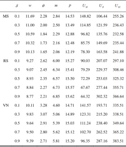
δ w θ m p UM UR USC
MS 0.1 11.69 2.28 2.84 14.53 148.82 106.44 255.26
0.3 11.00 2.00 2.50 13.49 114.85 121.59 236.43
0.5 10.59 1.84 2.29 12.88 96.82 135.76 232.58
0.7 10.32 1.73 2.16 12.48 85.75 149.69 235.44
0.9 10.13 1.65 2.06 12.19 78.30 163.58 241.88
RS 0.1 9.27 2.62 6.00 15.27 90.03 207.07 297.10
0.3 9.07 2.45 6.34 15.41 79.29 229.37 308.46
0.5 8.93 2.35 6.57 15.50 72.29 253.03 325.32
0.7 8.84 2.27 6.73 15.57 67.67 277.44 355.71
0.9 8.77 2.21 6.85 15.62 64.32 302.32 366.64
VN 0.1 10.11 3.28 4.60 14.71 141.57 193.71 335.51
0.3 9.83 3.07 5.06 14.89 123.31 215.20 338.51
0.5 9.64 2.91 5.39 15.03 111.24 238.40 349.64
0.7 9.50 2.80 5.62 15.12 102.70 262.52 365.22
0.9 9.39 2.71 5.81 15.20 96.35 287.16 383.51
Based on the results showed in Tables I, II and III, we find:
1) The wholesale price w is the highest in the MS game when the manufacturer has more bargaining power, followed by the VN and then the RS games. The greening level θ is the lowest in the MS game this is because under this game the full costs of investment
IAENG International Journal of Applied Mathematics, 48:4, IJAM_48_4_15
are afforded by the manufacturer. The profit margin of the retailer m is the highest in the RS game, followed by the VN and then the MS games.
2) The retailer sets the highest retail price in the MS game and the lowest in the VN game in Tables I and II, while the retail price is the highest in the RS game, followed by the VN and then the MS games in Table III.
3) The manufacturer obtains the largest utility in the MS game, and the smallest in the RS game in Tables I and III, while he obtains the largest utility in the VN game, and the smallest in the RS game in Table II. On the other hand, the retailer obtains the largest utility in the RS game, and the smallest in the MS game. It indicates that the actor who is the leader in the supply chain not always takes advantage in making the higher utility with reference effect and fairness concern. In addition, the supply chain system always obtains the largest utility in the VN game, followed by the RS and then the MS games.
4) When the reference price coefficient of the consumer λ increases, the wholesale price w, the greening level θ, the profit margin m and the retail price p are all decreasing in the three games. While the utilities of the manufacturer, the retailer and the supply chain system increase as the reference price coefficient λ increases.
5) When the retailer’s fairness concern coefficient δ increases, the wholesale price w, the greening level θ and the profit margin m decrease. The retailer price p decreases as the fairness concern parameter δ increases in the MS game, while the retailer price increases as the fairness concern coefficient δ increases in the RS and VN games. The utility of the manufacturer decreases as the fairness concern coefficient δincreases, while the utility of the retailer increases as the fairness concern coefficient δ increases. When the fairness concern coefficient δ increases, the utility of the supply chain system increases in the RS and VN games, while decreases first and then increase in the MS game.
6) The optimal policies in Table I show the results at 0
λ = andδ =0, which are just the optimal solutions without consideration of the reference price effect of the consumer and the fairness concern of the retailer. Compared these optimal solutions without reference price effect and fairness concerns to those with fairness reference price effect and fairness concerns, we observe that the wholesale price, the greening level, the profit margin and the retail price are higher than those with the reference price effect and the fairness concern. The utility of the retailer is higher in the three games, while the utility of the manufacturer is lower in the MS and RS games when the reference price effect and the fairness concerns are considered. It means that the retailer could benefit from the reference price effect and the fairness concern, while the manufacturer could suffer from this condition in the MS and RS games.
V. 4BCONCLUSION
This paper considers the pricing and greening level decisions in a green supply chain, where the manufacturer and retailer pursue three different kinds of scenarios: Manufacturer-Stackelberg game, Retailer-Stackelberg game and Vertical-Nash game. In our models the manufacturer is fairness neutral and the retailer is fairness sensitive. We also examine the effect of the reference price coefficient and the fairness concern coefficient on the prices, greening level and utilities of the manufacturer and the retailer, which is truly representative of the decision maker’s behavior.
Based on the discussions above, three findings can be obtained. Firstly, the reference price coefficient positively affects the utilities of the manufacturer, the retailer and the supply chain system. Secondly, the actor who dominates the supply chain not always takes advantage in making more utility with reference effect and fairness concern. Thirdly, the retailer can benefit in the three games, while the manufacturer can suffer in the MS and RS games with the reference price effect and the fairness concerns.
Our study mainly focus on one manufacturer and one retailer in a two-echelon green supply chain, therefore, the pricing and greening level decisions with multiple competitive manufacturers or retailers are the important directions for the future research.
REFERENCES
[1] D. Ghosh and J. Shah, “A comparative analysis of greening policies across supply chain structures”, International Journal of Production
Economics, vol. 135, no.2, pp. 568–583, 2012.
[2] G. Xie, W. Yue, W. Liu and S. Wang, “Risk based selection of cleaner products in a green supply chain”, Pacific Journal of Optimization, vol. 8, no.3, pp. 473–484, 2012.
[3] G. Xie, W. Yue and S. Wang, “Optimal selection of cleaner products in a green supply chain with risk aversion”, Journal of Industrial and Management Optimization, vol. 11, no.2, pp. 515–528, 2015. [4] G. Xie, “Modeling decision processes of a green supply chain with
regulation on energy saving level”, Computers & Operations
Research, vol. 54, pp. 266–273, 2015.
[5] P. Liu and S.P. Yi, “Pricing policies of green supply chain considering targeted advertising and product green degree in the Big Data
environment”, Journal of Cleaner Production, vol. 164,
pp.1614–1622, 2017.
[6] S. Swami and J. Shah, Channel coordination in green supply chain management, Journal of the Operational Research Society, vol. 64, no.3, pp. 336–351, 2013.
[7] C.T. Zhang and L.P. Liu, “Research on coordination mechanism in three-level green supply chain under non-cooperative game”, Applied
Mathematical Modelling, vol. 37, no.5, pp. 3369–3379, 2013. [8] C.T. Zhang, H.X. Wang and M. L. Ren, “Research on pricing and
coordination strategy of green supply chain under hybrid production mode”, Computers & Industrial Engineering, vol. 72, pp. 24–31, 2014.
[9] D. Ghosh and J. Shah, “Supply chain analysis under green sensitive consumer demand and cost sharing contract”, International Journal of Production Economics, vol. 164, pp. 319–329, 2015.
[10] Y. Huang, K. Wang, T. Zhang and C. Pang, “Green supply chain coordination with greenhouse gases emissions management: a game-theoretic approach”, Journal of Cleaner Production, vol. 112, pp. 2004–2014, 2016.
[11] Z. Basiri and J. Heydari, “A mathematical model for green supply chain coordination with substitutable products”, Journal of Cleaner Production, vol. 145, pp. 232–249, 2017.
[12] H. Song and X. Gao, “Green supply chain game model and analysis under revenue-sharing contract”, Journal of Cleaner Production, vol. 170, pp. 183–192, 2018.
[13] J.B. Sheu, “Bargaining framework for competitive green supply chains under governmental financial intervention”, Transportation Research
Part E : Logistics and Transportation Review, vol. 47, no.5, pp. 573–592, 2011.
IAENG International Journal of Applied Mathematics, 48:4, IJAM_48_4_15
[14] J.B. Sheu and Y.J. Chen, “Impact of government financial intervention on competition among green supply chains”, International Journal of Production Economics, vol. 138, no.1, pp. 201–213, 2012.
[15] B. Li, M. Zhu, Y. Jiang and Z. Li, “Pricing policies of a competitive dual-channel green supply chain”, Journal of Cleaner Production, vol. 112, pp.2029–2042, 2016.
[16] S. Chen, X. Wang, Y. Wu and Lin Li, “Pricing policies in green supply chains with vertical and horizontal competition”,
Sustainability, vol. 9, no. 12, pp. 1–23, 2017.
[17] A. Hafezalkotob, “Competition, cooperation, and coopetition of green supply chains under regulations on energy saving levels”,
Transportation Research Part E: Logistics and Transportation Review, vol. 97, pp. 228–250, 2017.
[18] W. Zhu, “Green product design in supply chains under competition”, European Journal of Operational Research, European Journal of
Operational Research, vol. 258, no.1, pp. 165–180, 2017.
[19] D. Yang and T. Xiao, “Pricing and green level decisions of a green supply chain with governmental interventions under fuzzy uncertainties”, Journal of Cleaner Production, vol. 149, pp. 1174–1187, 2017.
[20] S. Sang, Decentralized channel decisions of green supply chain in a fuzzy decision making environment, International Journal of Computational Intelligence Systems, vol. 10, no.1, pp.986–1001, 2017.
[21] T.H. Cui, J.S. Raju and Z.J. Zhang, “Fairness and Channel Coordination”, Management Science, vol. 53, no.8, pp.1303–1314, 2007.
[22] O. Caliskan-Demirag, Y. Chen and J. Li, “Channel coordination under fairness concerns and nonlinear demand”, European Journal of
Operational Research, vol. 207, no.3, pp.1321–1326, 2010. [23] J. Yang, J. Xie, X. Deng and H. Xiong, “Cooperative advertising in a
distribution channel with fairness concerns”, European Journal of Operational Research, vol. 227, no.2, pp. 401–407, 2013.
[24] S. Du, T. Nie, C. Chu and Y. Yu, “Newsvendor model for a dyadic supply chain with Nash bargaining fairness concerns”, International
Journal of Production Research, vol. 52, no.17, pp. 5070–5085, 2014. [25] T. Nie and S. Du, “Dual-fairness supply chain with quantity discount contracts”, European Journal of Operational Research, vol. 258, no.2, pp. 491–500, 2017.
[26] S. Sang, “Pricing and service decisions in a supply chain with fairness reference”, Engineering Letters, vol. 25, no.3, pp. 277–283, 2017. [27] J. Zhang, WK. Chiang and L. Liang, “Strategic pricing with reference
effects in a competitive supply chain”, Omega, vol. 44, no.2, pp. 126–135, 2014.
[28] Z. Lin, “Price promotion with reference price effects in supply chain”,
Transportation Research Part E, vol.85, pp. 52–68, 2016.
[29] J. Xu and N. Liu,“Research on closed loop supply chain with reference price effect”, Journal of Intelligent Manufacturing, vol. 28, no.1, pp. 51–64, 2017.
Shengju Sang is an associate professor at School of Business, Heze University, Heze, China. He received his Ph.D. degree in 2011 at the School of Management and Economics, Beijing Institute of Technology, China. His research interest includes supply chain management, fuzzy decisions and its applications. He is an author of several publications in these fields such as Fuzzy Optimization and Decision Making, Journal of Intelligent & Fuzzy Systems, International Journal of Computational Intelligence Systems, Springer Plus, Mathematical Problems in Engineering and other journals.