The New Estimations of Diagonally Dominant Degree and Eigenvalues Distributions for the Schur Complements of Block Diagonally Dominant Matrices and Determinantal Bounds

(1)

The New Estimations of Diagonally Dominant

Degree and Eigenvalues Distributions for the

Schur Complements of Block Diagonally

Dominant Matrices and Determinantal Bounds

Zhengge Huang, Ligong Wang

∗

, Zhong Xu, Jingjing Cui

Abstract—In this paper, some new estimations of diagonally dominant degree on the Schur complement of I(II)-block diago-nally dominant matrices are obtained by applying the properties of Schur complement and some inequality techniques, which improve some existing ones. Further, as an application, we present some new distribution theorems for eigenvalues of the Schur complement and some new upper and lower bounds for the determinant of I(II)-block diagonally dominant matrices. These results are proved to be sharper than some known ones. Finally, numerical examples are also presented to confirm the theoretical results studied in this paper.

Index Terms—block matrix, Schur complement, diagonally dominant degree, eigenvalue distribution, determinant.

I. INTRODUCTION

T

HE Schur complement has been proved to be a useful tool in many fields such as control theory, statistics and computational mathematics, and many works have been done on it (see [1], [2], [3], [4], [5], [6]). Applying the Schur-based iteration method mentioned in [7], [8], we can solve large scale linear systems though reducing the order by the Schur complement. That is, for a non-homogeneous system of linear equationM x=bwith a nonsingular leading principal submatrix. Partition M as

M =

A B

C D

,

where A is supposed to be nonsingular. Partition x = (xT

1, xT2)T and b = (bT1, bT2)T conformably with M. This linear equation can be formally regard as a special case of the saddle point problems [9] The linear systemM x=b is equivalent to the pair of linear systems

(

Ax1+Bx2=b1,

Cx1+Dx2=b2.

If we multiply the first equation by −CA−1 _{and add it to} the second equation, the vector variablex1is eliminated and

Manuscript received September 01, 2016; revised December 09, 2016. This work was supported by the National Natural Science Foundations of China (No. 11171273) and Innovation Foundation for Doctor Dissertation of Northwestern Polytechnical University (No. CX201628).

∗_{Ligong Wang, Corresponding Author, is with the Department of Applied} Mathematics, School of Science, Northwestern Polytechnical University, Xi’an, Shaanxi, 710072, PR China. e-mail: [email protected].

Zhengge Huang (e-mail: [email protected]), Zhong Xu (e-mail: [email protected]) and Jingjing Cui (e-mail: [email protected]) are with the Department of Applied Mathematics, School of Science, Northwestern Polytechnical University, Xi’an, Shaanxi, 710072, PR China.

we obtain a linear system of smaller size (D−CA−1B)x1=b2−CA−1b1.

If the coefficient matrixD−CA−1_B _{is a block diagonally} dominant matrix or a blockH-matrix, we can use some block or preconditioned iterative methods [10], [11] to continue resolving the linear system equation (1). In the meanwhile, when we solve linear equation system, the convergence rate of many iterate algorithms are closely related with spectral radius of coefficient matrix. Hu [12] obtained the following result which can be used to estimate the convergence rate:

LetM = (Mij)m×m be a block strictly diagonally

dom-inant matrix and N = (Nij)m×m partitioned conformably

withM. Then

ρ(M−1N)≤max

i

m P j=1

kNijk kM_ii−1k−1₋P j6=i

kMijk.

Therefore, we know the estimate of block matrix’s spec-tral is closely related with the block diagonally dominant degree kM_ii−1k−1 ₋ P

j6=i

kMijk of each row when M is

a block strictly diagonally dominant matrix. Thus, after being reduced order, it is significant to study the block diagonally dominant degree of the coefficient matrix of the linear equation system (1). Additionally, as mentioned in [13], we see that the eigenvalues of Schur complement of diagonally dominant matrix are more concentrated than those of original matrix, and we predict that the Schur-based conjugate gradient method will compute faster than the ordinary conjugate gradient method. Hence, it is very important to estimate the eigenvalue distributions of (block) diagonally dominant matrix. Over the years, there has been a surge of interest in studying the locations of eigenvalues of the Schur complement of matrices in much literature, see [6], [7], [8], [13], [14], [15], [16], [17], [18], [19], [20], [21]. Moreover, the determinant of matrices has hitherto great influence on every branch of mathematics [22], [23], [24], [25], [26]. Zhang and Liu [17] proposed some upper and lower bounds for determinants of diagonally dominant matrices by making use of the results of the estimates of diagonally dominant degree for the Schur complement of the diagonally dominant matrices. On the other hand, the authors in [27], [28], [29], [30] extended the concept of diagonally dominant matrix and developed two kinds of block diagonally dominant matrices, which are referred to as the I-block [27] and II-block [31] diagonally dominant

IAENG International Journal of Applied Mathematics, 47:2, IJAM_47_2_07

(2)

matrices, respectively. Later, two kinds of generalized block strictly diagonally dominant matrices (I-block [32](II-block [31]) H-matrices) are established in [31], [32], [33]. In the sequel, Liu et al. [13] derived some estimations of diagonally dominant degree and eigenvalue inclusion sets for the Schur complement of I(II)-block diagonally dominant matrices, and Wang [20], [21] put forward the new estimations of diagonally dominant degree and eigenvalue inclusion sets which are proved to be tighter than those of [13]. Zhu [34] obtained some upper and lower bounds for determinants of I(II)-block diagonally dominant matrices, and Xu [35] arrived at some determinants bounds are sharper than the ones obtained by Zhu. In the current work, we first focus on investigating the following three aspects:

• Study the new estimates of I(II)-block diagonally dom-inant degree for Schur complement of matrices. • Derive the new distributions for the eigenvalues of the

Schur complement of matrices.

• Develop the new upper and lower bounds for determi-nants of the I(II)-block diagonally dominant matrices. Afterward, we prove that the proposed results are superior to some known ones in theory. The numerical results are im-plemented to verify the theoretical results. Before presenting the our main results of this paper, we give some definitions which are used throughout this paper as follows.

Let Cn×n denote the set of all n×ncomplex matrices,

N ={1,2,· · · , n} andA= (aij)∈Cn×n(n≥2). Denote

τi(A) = X j6=i

|aij|, i∈N.

A= (aij)∈Cn×n is a strictly diagonally dominant matrix (abbreviated to SDn) if |aii|> τi(A), for i∈N.

The comparison matrix of A, denoted by µ(A) = (tij)n×n, is defined to be

tij = (

|aij|, if i=j, −|aij|, if i6=j.

A matrixAis called anM-matrix if there exist a nonnegative matrixBand a real numbers > ρ(B)such thatA=sI−B, where ρ(B) is the spectral radius of B. It is well known that A is anH-matrix if and only if µ(A)is anM-matrix, then the Schur complement of A is also an M-matrix and detA >0(see [14]).

Forα⊆N, denote by|α| the cardinality ofα andα0 = N −α. If α, β ⊆ N, then A(α, β) is the submatrix of A

lying in the rows indicated byαand the columns indicated byβ. In particular,A(α, α)is abbreviated to A(α). Assume that A(α) is nonsingular. Then

A/α=A/A(α) =A(α0)−A(α0, α)[A(α)]−1A(α, α0),

is called the Schur complement of Arespect to A(α). LetA∈Cn×n be partitioned as the following form:

A=

    

A(α1, α1) A(α1, α2) · · · A(α1, αs)

A(α2, α1) A(α2, α2) · · · A(α2, αs)

..

. ... . .. ...

A(αs, α1) A(αs, α2) · · · A(αs, αs)     

, (1)

where1≤s≤n,α0= 0,

αi= i−1

X t=0

|αt|+ 1,· · ·,

i X t=0

|αt|

(1≤i≤s),

i X t=0

|αt|=n

andA(αt, αt)is a|αt|×|αt|nonsingular principal submatrix

ofA,t= 1,2,· · · , s.

Without loss of generality, we assume thatCns×n denote

the set of all s ×s block matrices in Cn×n partitioned as (1), A = (A(αl, αm))sn×n ∈ Cns×n and N(A) =

(kA(αl, αm)k)sdenote the norm matrix of block matrixA.

In this paper, the matrix normk.kofA∈Cn×nis defined as

kAk= sup

x∈Cm,x6=0

kAxk kxk .

Thus ifA∈Cn×n is nonsingular, then it holds that

kA−1k−1=

sup

x∈Cm,x6=0

kA−1_x_k

kxk −1

= inf

x∈Cm,x6=0

kAxk kxk . (2)

Definition 1.1 A is called an I-block strictly diagonally dominant matrix (I−BSDs) [27] if for all1≤l≤s,

k[A(αl, αl)]−1k−1> s X m=1,m6=l

kA(αl, αm)k. (3)

Denote byk[A(αl, αl)]−1k−1− s P m=1,m6=l

kA(αl, αm)kthe

I-block diagonally dominant degree for1≤l≤sof A. Definition 1.2 A is called an II-block strictly diagonally dominant matrix (II−BSDs) [28] if for all 1≤l≤s,

s X m=1,m6=l

k[A(αl, αl)]−1A(αl, αm)k<1. (4)

1 −

s P m=1,m6=l

k[A(αl, αl)]−1A(αl, αm)k represents the

II-block diagonally dominant degree for 1 ≤ l ≤ s of A. It is noteworthy that if A ∈I−BSDs, then it follows from

(3), (4) and the inequality

kA(αl, αl)A(αl, αm)k ≤ kA(αl, αl)kkA(αl, αm)k

thatA∈II−BSDs.

Definition 1.3 A is called an I-block H-matrix and II -blockH-matrix, respectively, if the comparison matrices of block matrix A which are defined by µI(A) = (ωl,m) ∈ Rs×sandµII(A) = (¯ωl,m)∈Rs×s areM-matrix, where

ωl,m=

k[A(αl, αl)]−1k−1, if l=m, −kA(αl, αm)k, if l6=m,

¯ ωl,m=

1, if l=m,

−k[A(αl, αl)]−1A(αl, αm)k, if l6=m.

The remainder of this paper is organized as follows. In Section II, we recollect some useful lemmas which are uti-lized in the next sections. Several new estimates for the I(II)-block diagonally dominant degree of the Schur complement of matrices are established in Section III. As applications, some new distribution theorems for eigenvalues of the Schur complement and the new bounds for the determinant of I(II)-block diagonally dominant matrices are obtained in Section IV and Section V, respectively. Section VI is devoted to performing some numerical experiments to confirm the advantages and the validity of the established results. Finally, the paper is ended with some conclusions in Section VII.

IAENG International Journal of Applied Mathematics, 47:2, IJAM_47_2_07

(3)

II. PRELIMINARIES

In this section, we start with some lemmas. They will be useful in the following proofs.

Lemma 2.1 [13] If A ∈ SDn, then µ(A) is M-matrix,

i.e.,A isH-matrix.

Lemma 2.2 [2] If A is a H-matrix, then [µ(A)]−1 ≥ |A−1|.

Lemma 2.3 [30] If A ∈ I−BSDs, then [µI(A)]−1 ≥

N(A−1₎_.

Lemma 2.4 [30] If A ∈ II−BSDs,

then [µII(A)]−1 ≥ N(A−1D), where D =

diag(A(α1, α1), A(α2, α2),· · ·, A(αs, αs)).

Lemma 2.5 Let A ∈ Cns×n, α = k S u=1

αiu ⊂ N, α

0 ₌

N −α=

l S v=1

αjv ⊂N, and k+l =s. For any αjt ⊂α

0_, we denote:

Bjt =

x −Gt

−HT µ˜[A(α)]

.

IfA∈I−BSDs, we takeµ˜[A(α)] =µI[A(α)],

Gt={kA(αjt, αi1)k,· · ·,kA(αjt, αik)k},

H=

l

X u=1

kA(αi1, αju)k,· · · , l X u=1

kA(αik, αju)k

.

If

x≥h

k X v=1

kA(αjt, αiv)k

Piv(A) k[A(αiv, αiv)]

−1_k−1, (5) where

r= max

1≤w≤k

l

P

v=1

kA(αiw, αjv)k

k[A(αiw, αiw)]−1k−1− k

P

t=1,t6=w

kA(αiw, αit)k

,

Piw(A) =r k

X

t=1,t6=w

kA(αiw, αit)k+ l

X

v=1

kA(αiw, αjv)k,

h= max

1≤w≤k l

P

v=1

kA(αiw, αjv)k

Hi

, Hi=Piw(A)−

k

X

t=1,t6=w

kA(αiw, αit)k

Pit(A)

k[A(αit, αit)] −1_k−1,

thendetBjt >0. If A∈II−BSDs, we takeµ˜[A(α)] =

µII[A(α)],

Gt = {k[A(αjt, αjt)]

−1_A₍_α

jt, αi1)k, · · ·,k[A(αjt, αjt)]

−1_A₍_α

jt, αik)k},

H =

l

X u=1

k[A(αi1, αi1)]−1A(αi1, αju)k,

· · ·,

l X u=1

k[A(αik, αik)]

−1_A₍_α

ik, αju)k

.

If

x≥f

k X v=1

k[A(αjt, αjt)]

−1_A₍_α

jt, αiv)kP˜iv(A), (6)

where

η= max

1≤w≤k l

P

v=1

k[A(αiw, αiw)]−1A(αiw, αjv)k

1− Pk

t=1,t6=w

k[A(αiw, αiw)] −1_A₍_α

iw, αit)k ,

˜

Piw(A) =η k

X

t=1,t6=w

k[A(αiw, αiw)]−1A(αiw, αit)k

+ l

X

v=1

k[A(αiw, αiw)]−1A(αiw, αjv)k,

f= max

1≤w≤k l

P

v=1

iw, αjv)k Gi

,

Gi= ˜Piw(A)− k

X

t=1,t6=w

iw, αit)kP˜it(A),

thendetBjt >0.

Proof. If strict inequality in (5) holds, we take ε > 0, sufficiently small such that

x >

k X v=1

kA(αjt, αiv)k

h Piv(A) k[A(αiv, αiv)]

−1_k−1 +ε

.

We construct a positive diagonal matrix D = diag(d1, d2,· · · , dk+1), where

dv = (

1, v= 1,

h Piv−1(A)

k[A(α_iv₋₁,α_iv₋₁)]−1_k−1 +ε, 2≤v≤k+ 1.

DenoteCt=BjtD= (csv)(k+1)×(k+1). Ifs= 1, then

|css| − k+1 X v=1,v6=s

|csv|=|c11| −

k+1 X v=2

|c1v|

=x−

k X v=1

kA(αjt, αiv)k

h Piv(A) k[A(αiv, αiv)]

−1_k−1 +ε

>0;

Ifs= 2,3,· · · , k+ 1, then it has

|css| − k+1

X

v=1,v6=s

|csv|

= k[A(αis−1, αis−1)]

−1_k−1₍_h Pis−1(A)

k[A(αis−1, αis−1)]−1k−1

+ε)

−

l

X

u=1

kA(αis−1, αju)k

−

k

X

w=1,w6=s−1

kA(αis−1, αiw)k(h

Piw(A)

k[A(αiw, αiw)]−1k−1 +ε)

= hPis−1(A) +εk[A(αis−1, αis−1)] −1_k−1₋

l

X

u=1

kA(αis−1, αju)k

−

k

X

w=1,w6=s−1

kA(αis−1, αiw)k(h

Piw(A)

k[A(αiw, αiw)]−1k−1 +ε).(7)

Since A∈I−BSDs, it holds that0 ≤r <1. Moreover,

for1≤u≤k, we have

r≥

l P v=1

kA(αiu, αjv)k

k[A(αiu, αiu)]−

1_k−1₋

k P t=1,t6=u

kA(αiu, αit)k

,

IAENG International Journal of Applied Mathematics, 47:2, IJAM_47_2_07

(4)

i.e.,

rk[A(αiu, αiu)]

−1_k−1_≥

l X v=1

kA(αiu, αjv)k

+r

k X t=1,t6=u

kA(αiu, αit)k=Piu(A).

From the above inequality, for1≤u≤k, we obtain

0≤ Piu(A)

k[A(αiu, αiu)]

−1_k−1 ≤r <1. By the definition of Piw(A), for 1≤w≤k, we have

l P v=1

kA(αiw, αjv)k

Piw(A)− k P t=1,t6=w

kA(αiw, αit)k

P_it(A) k[A(α_it,α_it)]−1_k−1

=

Piw(A)−r k P t=1,t6=w

kA(αiw, αit)k

Piw(A)− k P t=1,t6=w

kA(αiw, αit)k

≤ 1,

which leads to 0≤h≤1. Furthermore, for1≤u≤k,

h≥

l P v=1

kA(αiu, αjv)k

Piu(A)− k P t=1,t6=u

kA(αiu, αit)k

,

which can be rewritten as

hPiu(A)≥ l X v=1

kA(αiu, αjv)k

+h

k X t=1,t6=u

kA(αiu, αit)k

Pit(A) k[A(αit, αit)]−

1_k−1. Thus, it follows from Equality (7) that fors= 2,3,· · · , k+1,

|css| − k+1 X

v=1,v6=s

|csv|

= hP_is₋₁(A) +εk[A(α_is₋₁, α_is₋₁)]−1k−1−

l X

u=1

kA(α_is₋₁, αju)k

−

k X

w=1,w6=s−1

kA(α_is₋₁, α_iw)k(h Piw(A) k[A(αiw, αiw)]−1k−1

+ε)

≥

l X

u=1

kA(α_is₋₁, αju)k+h k X

w=1,w6=s−1

kA(α_is₋₁, αiw)k

× Piw(A)

k[A(α_iw, α_iw)]−1_k−1+εk[A(αis−1, αis−1)] −1

k−1

−

l X

u=1

kA(α_is₋₁, αju)k

−

k X

w=1,w6=s−1

kA(α_is₋₁, αiw)k(h

Piw(A)

k[A(α_iw, α_iw)]−1_k−1+ε)

= ε

k[A(α_is₋₁, α_is₋₁)]−1k−1−

k X

w=1,w6=s−1

kA(α_is₋₁, α_iw)k

>0,

which means that Ct is a SDk+1. By Lemma 2.1,µ(Bjt)

is aM-matrix. Note thatµ(Bjt) =Bjt, thendetBjt >0.

When the equality holds in (5), for any ε > 0, denote

Bε=B+ diag(ε,0,· · ·,0). In a similar way to the above

proof, we have Bε ∈ SDk+1 and hence detBjt > 0. Let

ε→0+_{, we get}_det_B

jt ≥0immediately.

For the case ofA∈II−BSDs, the proof is similar.

Lemma 2.6 [30] Let A ∈ I−(II−)BSDs, α = k

S u=1

αiu ⊂ N, α

0 ₌ _N ₋_α ₌ Sl v=1

αjv, and k+l = s.

For anyt= 1,2,· · ·, l,,

Ψt= 1−

[A(αjt, αjt)] −1

[A(αjt, αi1),

· · ·, A(αjt, αik)][A(α)] −1



 

A(αi1, αjt)

.. .

A(αik, αjt)



 

>0.

Lemma 2.7[2] LetA∈Cn×n. IfkAk<1, thenIn−A

is nonsingular and

k(In−A)−1k ≤

1 1− kAk.

whereIn is an identity matrix.

III. THE DIAGONALLY DOMINANT DEGREE FORSCHUR COMPLEMENT

In this section, we present several new estimates on the block diagonally dominant degree of the Schur complement ofI−(II−)BSDs, which improve the corresponding ones

in [13], [20], [21], [35].

Theorem 3.1 Let A ∈ I−BSDs, α = k S u=1

αiu ⊂ N,

α0 = N −α =

l S v=1

αjv, and k+l = s. Denote A/α =

( ˜A(αt, αr)). Then

k[ ˜A(αt, αt)]−1k−1−Rt(A/α) ≥ k[A(αjt, αjt)]

−1_k−1₋_R

jt(A) +wjt ≥ k[A(αjt, αjt)]

−1_k−1₋_R

jt(A)>0 (8)

and

k[ ˜A(αt, αt)]−1k−1+Rt(A/α) ≤ k[A(αjt, αjt)]

−1_k−1₊_R

jt(A)−wjt ≤ k[A(αjt, αjt)]

−1_k−1₊_R

jt(A), (9)

where

Rjt = s X m=1,m6=jt

kA(αjt, αm)k,

wjt = k X v=1

kA(αjt, αiv)k

k[A(αiv, αiv)]

−1_k−1₋_hP

iv(A) k[A(αiv, αiv)]

−1_k−1 , andhandPiv(A) (v= 1,2,· · ·, k)are defined as in Lemma

2.5. Proof.Let

Ψtr = (A(αjt, αi1),· · ·, A(αjt, αik))[A(α)] −1



 

A(αi1, αjr)

.. .

A(αik, αjr)



 ,

Gt= (kA(αjt, αi1)k,· · ·,kA(αjt, αik)k) T

, H0=

l X

r=1

kA(αi1, αjr)k,· · ·, l

X

r=1

kA(αik, αjr)k

T

, t, r= 1,2,· · ·, l.

IAENG International Journal of Applied Mathematics, 47:2, IJAM_47_2_07

(5)

By the definition of Schur complement, denote byJt=|αjt|

and Im the identity matrix. According to Lemma 2.5, we

obtain ||[A(αjt, αjt)]

−1_Ψ

tt||<1. It follows that

k[ ˜A(αt, αt)]−1k−1− l

X

r=1,r6=t

k_A˜₍_α_t_{, α}_r₎k

= k{A(αjt, αjt)−Ψtt}−1k−1− l

X

r=1,r6=t

kA(αjt, αjr)−Ψtrk

≥ k[A(αjt, αjt)]

−1_k−1_k{_I

jt−[A(αjt, αjt)] −1_Ψ

tt}−1k−1

−

l

X

r=1,r6=t

≥ k[A(αjt, αjt)] −1_k−1h

1− k[A(αjt, αjt)] −1_Ψ

ttk

i

−

l

X

r=1,r6=t

kA(αjt, αjr)k − l

X

r=1,r6=t

kΨtrk

= k[A(αjt, αjt)]

−1_k−1_{− k}_[_A₍_α

jt, αjt)]

−1_k−1_k_[_A₍_α

jt, αjt)] −1_Ψ

ttk

−

l

X

r=1,r6=t

X

r=1,r6=t

kΨtrk

≥ k[A(αjt, αjt)]

−1_k−1_{− k}_Ψ

ttk

−

l

X

r=1,r6=t

X

r=1,r6=t

kΨtrk

= k[A(αjt, αjt)] −1_k−1₋

l

X

r=1,r6=t

X

r=1

kΨtrk

≥ k[A(αjt, αjt)] −1_k−1₋

l

X

r=1,r6=t

kA(αjt, αjr)k −G T

tN[(A(α)) −1_]_H0

≥ k[A(αjt, αjt)]−1k−1− l

X

r=1,r6=t

kA(αjt, αjr)k

−GTt[µI(A)(α)]−1H0(by Lemma 2.2)

= k[A(αjt, αjt)]

−1_k−1₋_R

jt(A) +wjt+ k

X

r=1

kA(αjt, αir)k

−wjt−GTt[µI(A)(α)]−1H0 = k[A(αjt, αjt)]

−1_k−1₋_R

jt(A) +wjt−ε

+ 1

det[µI(A)(α)] det





k

P

r=1

kA(αjt, αir)k −wjt+ε −GTt

−H0 _µ

I(A)(α)





= k[A(αjt, αjt)]

−1_k−1₋_R

jt(A) +wjt−ε+

detB1

det[µI(A)(α)] . (10)

Inasmuch asA∈I−BSDs, we have k

X r=1

kA(αjt, αir)k −wjt+ε

=h

k X r=1

kA(αjt, αir)k

Pir(A) k[A(αir, αir)]

−1_k−1+ε

> h

k X r=1

kA(αjt, αir)k

Pir(A) k[A(αir, αir)]−

1_k−1.

It follows that detB1 > 0 by virtue of Lemma 2.5. By Lemma 2.1, we infer that µI(A)(α) is M-matrix, and

thereforedet[µI(A)(α)]>0, which implies that

k[ ˜A(αt, αt)]−1k−1−Rt(A/α)

>k[A(αjt, αjt)]

−1_k−1₋_R

jt(A) +wjt−ε ≥ k[A(αjt, αjt)]

−1

k−1−Rjt(A)−ε.

Letε→0, thus we easily get

k[ ˜A(αt, αt)]−1k−1−Rt(A/α) ≥ k[A(αjt, αjt)]

−1_k−1₋_R

jt(A) +wjt ≥ k[A(αjt, αjt)]

−1

k−1−Rjt(A)>0,

which implies Inequality (8).

By making use of (2) and applying the same manner in the above proof, it has

k[ ˜A(αt, αt)]−1k−1+ l

X

r=1,r6=t

kA˜(αt, αr)k

= k{A(αjt, αjt)−Ψtt} −1

k−1+

l

X

r=1,r6=t

= inf

x∈Cm,x6=0

k{A(αjt, αjt)−Ψtt}xk

kxk

+

l

X

r=1,r6=t

kA(αjt, αjr)−Ψtrk(by (4))

≤ inf

x∈Cm,x6=0

kA(αjt, αjt)xk+kΨttxk

kx||

+

l

X

r=1,r6=t

kA(αjt, αjr)k+ l

X

r=1,r6=t

kΨtrk

≤ inf

x∈Cm,x6=0

kA(αjt, αjt)xk+kΨttkkxk

kxk

+

l

X

r=1,r6=t

kA(αjt, αjr)k+ l

X

r=1,r6=t

kΨtrk

= inf

x∈Cm,x6=0

kA(αjt, αjt)xk

kx||

+

l

X

r=1,r6=t

kA(αjt, αjr)k+ l

X

r=1 kΨtrk

= k[A(αjt, αjt)] −1_k−1

+

l

X

r=1,r6=t

kA(αjt, αjr)k

+

l

X

r=1

kΨtrk(by (4))

≤ k[A(αjt, αjt)] −1_k−1

+Rjt(A)−wjt+ε

− 1

det[µI(A)(α)]

detB1(by (10))

< k[A(αjt, αjt)] −1

k−1+Rjt(A)−wjt+ε

≤ k[A(αjt, αjt)] −1

k−1+Rjt(A) +ε.

Letε→0, thus we can get

k[ ˜A(αt, αt)]−1k−1+Rt(A/α) ≤ k[A(αjt, αjt)]

−1_k−1₊_R

jt(A)−wjt ≤ k[A(αjt, αjt)]

−1_k−1₊_R

jt(A).

Therefore, we obtain Inequality (9). This proof is completed.

Remark 3.1Note that

h Piu(A) k[A(αiu, αiu)]

−1_k−1 ≤

Piu(A) k[A(αiu, αiu)]

−1_k−1

≤r≤ max 1≤u≤k

Riu(A) k[A(αiu, αiu)]

−1_k−1, 1≤u≤k.

IAENG International Journal of Applied Mathematics, 47:2, IJAM_47_2_07

(6)

This means that

wjt = k

X

v=1

kA(αjt, αiv)k

k[A(αiv, αiv)]

−1_k−1₋_hP

iv(A)

k[A(αiv, αiv)]−1k−1

≥

k

X

v=1

kA(αjt, αiv)k

k[A(αiv, αiv)]

−1_k−1₋_P

iv(A)

k[A(αiv, αiv)]−1k−1

≥ (1−r)

k

X

v=1

kA(αjt, αiv)k

= min

1≤u≤k

k[A(αiu, αiu)]−1k−1−Riu(A)

k[A(αiu, αiu)]−1k−1− k

P

t=1,t6=u

kA(αiu, αit)k

×

k

X

v=1

kA(αjt, αiv)k

≥ min

1≤u≤k

k[A(αiu, αiu)]

−1_k−1₋_R

iu(A)

k[A(αiu, αiu)]−1k−1 k

X

v=1

kA(αjt, αiv)k.

(11)

From Inequality (11), it’s obvious that Theorem 1 improves the results of Theorem 3.1 in [13], Theorem 2.10 in [21] and Theorem 2.1.1 in [35].

Based on Theorem 3.1, the following corollary can be obtained immediately.

Corollary 3.1 Let A ∈ I−BSDs, and take α = s−1

S u=1

αu⊂N. Then

k(A/α)−1k−1≥ k[A(αs, αs)]−1k−1 −h

s−1 X v=1

kA(αs, αv)k

Pv(A) k[A(αv, αv)]−1k−1

,

kA/αk ≤ kA(αs, αs)k

+h

s−1 X v=1

kA(αs, αv)k

.

Proof.Notice thatα0 =αs. Thus,A/α= ( ˜A(αs, αs)), and

Rs(A/α) = 0, so by the definition of wjt, we have

wjt =ws

=

s−1 X v=1

kA(αs, αv)k

k[A(αv, αv)]−1k−1−hPv(A) k[A(αv, αv)]−1k−1

=

s−1 X v=1

kA(αs, αv)k −h s−1 X v=1

kA(αs, αv)k

.

(12)

Substituting Equation (12) into Inequality (8) and in a manner similar to that done for Theorem 3.1, the results are

derived.

Theorem 3.2 Let A ∈II−BSDs, α= k S u=1

αiu ⊂N,

α0 = N −α =

l S v=1

αjv, and k+l = s. Denote A/α =

( ˜A(αt, αr)). Then

1−Rˆt(A/α)≥1−Rˆjt(A) + ˆwjt≥1−Rˆjt(A)>0(13)

and

1 + ˆRt(A/α)≤1 + ˆRjt(A)−wˆjt ≤1 + ˆRjt(A), (14)

where

ˆ

Rjt(A) = s X m=1,m6=jt

k[A(αjt, αjt)]

−1_A₍_α

jt, αm)k,

ˆ wjt =

k X v=1

k[A(αjt, αjt)]

−1_A₍_α

jt, αiv)k(1−fP˜iv(A)),

andf andP˜iv(A) (v= 1,2,· · ·, k)are defined as in Lemma

2.4.

Proof.Fort, r= 1,2,· · ·, l, denoteJt=|αjt|, let D= diag(A(αi1, αi1),· · ·, A(αik, αik)),

Ψtr= (A(αjt, αi1),· · ·, A(αjt, αik))[A(α)]−1 

  

A(αi1, αjr) . . . A(α_ik, αjr)



   ,

Υt=[A(αjt, αjt)]−1A(αjt, αi₁),· · ·,[A(αjt, αjt)]−1A(αjt, αik) ,

Γr=[A(αi1, αi1)] −1

A(αi1, αjr),· · ·,[A(αik, αik)]−1A(αik, αjr) T, Lt=k[A(αjt, αjt)]−1A(αjt, αi1)||,

· · ·,k[A(α_jt, α_jt)]−1A(α_jt, α_ik)k T,

H0=

l X

r=1

k[A(αi1, αi1)] −1_A₍_α

i1, αjr)k,

· · ·, l X

r=1

||[A(α_ik, α_ik)]−1A(α_ik, α_jr)k T

.

It follows from the definition ofΨtin Lemma 2.6 that

Ψt= 1− k[A(αjt, αjt)]

−1

Ψttk= 1− kΥt[A(α)]−1DΓtk,

which is equivalent to

1 Ψt

[1− kΥt[A(α)]−1DΓtk] = 1. (15)

According to lemma 2.7, we obtain

Ijt−[A(αjt, αjt)]

−1_Ψ

tt −1

≤ 1

1− k[A(αjt, αjt)]

−1_Ψ

ttk

= 1

Ψt

. (16)

By making use of the definition of the Schur complement, we deduce that

1−Rˆt(A/α) = 1− l

X

r=1,r6=t

k[ ˜A(αt, αt)]−1A˜(αt, αr)k

= 1−

l

X

r=1,r6=t

k[A(αjt, αjt)−Ψtt] −1_[_A₍_α

jt, αjr)−Ψtr]k

= 1−

l

X

r=1,r6=t

Ijt−[A(αjt, αjt)]−1Ψtt −1

×

[A(αjt, αjt)]−1A(αjt, αjr)−[A(αjt, αjt)]−1Ψtr

≥1−

l

X

r=1,r6=t

Ijt−[A(αjt, αjt)] −1_Ψ

tt −1

[A(αjt, αjt)] −1_A₍_α

jt, αjr)−Υt[A(α)] −1_D_Γ

t

≥1− 1 Ψt

l

X

r=1,r6=t

k[A(αjt, αjt)]−1A(αjt, αjr)k

+kΥtkk[A(α)]−1DkkΓtk (by (16))

= 1 Ψt

(

1− kΥt[A(α)]−1DΓtk

IAENG International Journal of Applied Mathematics, 47:2, IJAM_47_2_07

(7)

−

l

X

r=1,r6=t

k[A(αjt, αjt)] −1_A₍_α

jt, αjr)k

−

l

X

r=1,r6=t

kΥtkk[A(α)]−1DkkΓt||

)

(by (15))

≥ 1 Ψt

(

1−

l

X

r=1,r6=t

−

l

X

r=1

kΥtkN[(A(α))−1D]kΓtk

)

≥ 1−

l

X

r=1,r6=t

−LTt{µII[A(α)]}−1H0(by Lemma 2.4)

= 1−_Rˆ_jt₍_A_{) + ˆ}_w_jt₊ k

X

r=1

k[A(αjt, αjt)]−1A(αjt, αir)k

−wˆjt−L T

t{µII[A(α)]}−1H0 = 1−Rˆjt(A) + ˆwjt−ε+

1 det[µII(A)(α)]

× det





k

P

r=1

k[A(αjt, αjt)]−1A(αjt, αir)k −wˆjt+ε −LTt

−H0 _µ

II[A(α)]





= 1−_Rˆ_j

t(A) + ˆwjt−ε+

detB2

det[µII(A)(α)]

. (17)

Since A∈II−BSDs, it holds that

k X r=1

k[A(αjt, αjt)]

−1_A₍_α

jt, αir)k −wˆjt+ε

= f

k X r=1

k[A(αjt, αjt)]

−1_A₍_α

jt, αir)kP˜ir(A) +ε

> f

k X r=1

k[A(αjt, αjt)]

−1_A₍_α

jt, αir)kP˜ir(A).

By Lemma 2.3, it is easy to see thatdetB2>0. By Lemma 2.1, we deduce thatµII(A)(α)is nonsingularM-matrix, thus

det[µII(A)(α)]>0, which yields that

1−Rˆt(A/α)>1−Rˆjt(A) + ˆwjt−ε≥1−Rˆjt(A)−ε.

Letε→0, thus we can get

1−Rˆt(A/α)≥1−Rˆjt(A) + ˆwjt ≥1−Rˆjt(A)>0,

which proves the desired Inequality (13). We can prove Inequality (14) with a quite similar strategy utilized in this

theorem.

Remark 3.2Note that

fP˜iu(A)≤P˜iu(A)≤η≤ max

1≤u≤k

ˆ

Riu(A), 1≤u≤k,

which leads to

ˆ

wjt = k

X

v=1

k[A(αjt, αjt)] −1

A(αjt, αiv)k(1−fP˜iv(A))

≥

k

X

v=1

A(αjt, αiv)k(1−P˜iv(A))

= min

1≤u≤k

1−_Rˆ_iu₍_A₎ 1−

k

P

t=1,t6=u

k[A(αiu, αiu)]−1A(αiu, αit)k

×

k

X

v=1

A(αjt, αiv)k

≥ min

1≤u≤k(1−

ˆ

Riu(A)) k

X

v=1

A(αjt, αiv)k.

(18)

Evidently, from Inequality (18) we see that Theorem 2 improves the results of Theorem 3.2 in [13], Theorem 2.1.2 in [35] and Theorem 2.13 in [21].

IV. DISTRIBUTION FOR EIGENVALUES OF THESCHUR COMPLEMENT OFI-(II-)BSDs

In this section, as an application of our results in Section II and Section III, we establish some new locations for the eigenvalues of the Schur complements ofI−(II−)BSDs

by the elements of the original matrix. Without loss of generality, we assume thatα=

k S u=1

αiu ⊂N,α

0₌_N₋_α₌ l

S v=1

αjv ⊂ N, and k+l = s. Let A/α = ( ˜A(αr, αr)), |αt| =t andIt be the identity matrix. Denote by λ(A/α)

andλ(A)the set of eigenvalues ofA/αandA, respectively. Lemma 4.1 [13] Let A ∈ I−BSDs and λ(A) denote

the set of eigenvalues ofA. Then

λ(A)⊂G=

s [ i=1

[Gi∪λ(A(αi, αi))],

where

Gi=

λ: λ*λ(A(αi, αi)) and

k[A(αi, αi)−λI(αi)]−1k−1≤ s

X

k6=i

kA(αi, αk)k

.

Theorem 4.1LetA∈I−BSDs andwjt be defined as

in Theorem 3.1. Then

λ(A)⊂G=

s [ t=1

[Gt∪λ(A(αjt, αjt))],

where

Gi=

λ: λ_*λ(A(αjt, αjt)) and

k[λIjt−A(αjt, αjt)]

−1

k−1≤Rjt(A)−wjt

.

Proof. Let Ψtr be such as in Theorem 3.1. If λ *

λ[ ˜A(αt, αt)] and λ * λ[A(αjt, αjt)], then combining

In-IAENG International Journal of Applied Mathematics, 47:2, IJAM_47_2_07

(8)

equality (4) with Lemma 4.1 results in

k[λIt−A˜(αt, αt)]−1k−1

=

sup

x∈Cm,x6=0

k[λIt−A˜(αt, αt)]−1xk kxk

−1

= inf

x∈Cm,x6=0

k[λIt−A˜(αt, αt)]xk

kxk (by (4))

= inf

x∈Cm,x6=0

k{λIjt−[A(αjt, αjt)−Ψtt]}xk kxk

≥ inf

x∈Cm,x6=0

k[λIjt−[A(αjt, αjt)]xk

kxk −x∈Csupm,x6=0

kΨttxk kxk

=k[λIjt−[A(αjt, αjt)]

−1_k−1_{− k}_Ψ_ttk_. Moreover,

k[λIjt−[A(αjt, αjt)]

−1

k−1 ≤ k[λIt−[A(αt, αt)]−1k−1+kΨttk ≤ Rt(A/α) +kΨttk

=

l X r=1,r6=t

kA(αjt, αjr)−Ψtrk+kΨttk

≤ l X r=1,r6=t

kA(αjt, αjr)k+ l X r=1

kΨtrk

≤ Rjt(A)−wjt− k X r=1

kA(αjt, αir)k

+wjt+G T

t[µI(A)(α)]−1H0

= Rjt(A)−wjt+ε−

1 det[µI(A)(α)]

×det

 

k P r=1

kA(αjt, αir)k −wjt+ε −G T t

−H0 µI(A)(α)  

= Rjt(A)−wjt+ε−

detB1 det[µI(A)(α)]

,

whereH0,B1 andµI(A)(α)are defined as in the proof of

Theorem 3.1. ThusdetB1>0 anddet[µI(A)(α)]>0. So k[λIjt−[A(αjt, αjt)]

−1_k−1_{< R}

jt(A)−wjt+ε,

Letting ε→0 yields

−1_k−1_≤_R

jt(A)−wjt.

Ifλ⊆λ[ ˜A(αt, αt)]andλ*λ[A(αjt, αjt)], we assume that

˜

x6= 0is the eigenvector of Acorresponding to λ. Then 0 = k[λIt−

˜

A(αt, αt)]xk kx˜k

≥ inf

x∈Cm,x6=0

k[λIt−A˜(αt, αt)]xk kxk

= inf

x∈Cm,x6=0

k[λIt−A(αjt, αjt) + Ψtt]xk kxk

≥ inf

x∈Cm,x6=0

k[λIt−A(αjt, αjt)]xk − kΨttxk kxk

≥ inf

x∈Cm,x6=0 _k_[_λI

jt−A(αjt, αjt)]xk

kxk −

kΨttxk kxk

= inf

x∈Cm,x6=0

k[λIjt−A(αjt, αjt)]xk

kxk − kΨttxk

= k[λIjt−A(αjt, αjt)]

−1

k−1− kΨttk(by (4)).

Therefore,

−1_k−1

≤ kΨttk ≤Rt(A/α) +kΨttk ≤Rjt(A)−wjt,

which proves this theorem.

Remark 4.1 By Remark 3.1, it is obvious that Theorem 4.1 improves the results of Theorem 4.1 in [13], Theorem 3.1.1 in [35] and Theorem 3.5 in [21].

By Theorem 3.2, similar to the proof of Theorem 4.1, the following theorem can be derived.

Theorem 4.2LetA∈II−BSDsandwjt be defined as

in Theorem 3.2. Then

λ(A)⊂G=

s [ t=1

[Gt∪λ(A(αjt, αjt))],

where

Gi=

λ: λ_*λ(A(αjt, αjt)) and

k[λIjt−A(αjt, αjt)]

−1_k−1_≤_Υ

t

andΥt=kA(αjt, αjt)k[ ˆRjt(A)−wjt].

Remark 4.2Similar to the discussions in Remark 3.2, it can be seen that the results of Theorem 4.2 improve those in Theorem 4.2 of [13], Theorem 3.12 of [35] and Theorem 3.6 of [21].

V. SOME NEW BOUNDS FOR DETERMINANTS OF I-(II-)BSDs

In this section, we make use of the results in Sections II-IV to exhibit some new upper and lower bounds for the determinants ofI−(II−)BSDs.

Lemma 5.1[36] Let A= (aij)n×n,∅ 6=α⊆N, assume

thatA(α)is nonsingular. Then

detA= detA(α) detA/α.

Lemma 5.2 [29] Let A ∈ II−BSDs, then D−1A ∈

I−BSDs, whereD is defined as in Lemma 2.4.

Let {j1, j2,· · ·, js} be a rearrangement of the elements in{1,2,· · ·, s}. Denoteβ1 =αjs, β2 =αjs∪αjs−1, · · ·,

αs=αjs∪αjs−1∪· · ·∪αj1 =N. Thenβs−t+1−βs−t=αjt,

t= 1,2,· · · , s,β0=∅, and

Rjt[A(βs−t+1)] =

X αu⊂βs−t

kA(αjt, αu)k,

ˆ

Rjt[A(βs−t+1)] =

X αu⊂βs−t

k[A(αjt, αjt)]

−1

A(αjt, αu)k.

Let ϕ represent any rearrangement {j1, j2,· · · , js} of the elements in{1,2,· · · , s} withβ1, β2,· · ·, βsdefined as

above. Next, we establish some bounds for determinants of I-(II-)BSDsin the following theorems.

Theorem 5.1 Let A ∈ I−BSDs and be partitioned as

in (1). Then

|detA| ≥max

ϕ s Y t=1

k[A(αjt, αjt)]

−1_k−1₋_Θ

jt

|α_jt| (19)

and

|detA| ≤min

ϕ s Y t=1

{kA(αjt, αjt)k+ Θjt}

|α_jt|

, (20)

IAENG International Journal of Applied Mathematics, 47:2, IJAM_47_2_07

(9)

where

Θjt =h[A(βs−t+1)] X

αv∈βs−t

kA(αjt, αv)||

Pv[A(βs−t+1)] k[A(αv, αv)]−1k−1

,

r[A(βs−t+1)] = max

t+1≤u≤s

kA(αju, αjt)k

Ki

, Ki=k[A(αju, αju)]

−1 k−1−

s

X

v=t+1,v6=u

kA(αju, αjv)k,

Pjv[A(βs−t+1)] =r[A(βs−t+1)]

s

X

u=t+1,u6=v

||A(αjv, αju)k

+kA(αjv, αjt)k, αv∈βs−t,

h[A(βs−t+1)] = max

t+1≤u≤s

kA(αju, αjt)k

Li

, Li=Pju[A(βs−t+1)]

−

n

X

v=k+1,v6=u

kA(αju, αjv)||

Pjv[A(βs−t+1)] k[A(αjv, αjv)]−1k−1

.

Proof. Inasmuch as βs−t is contained in βs−t+1 and

βs−t+1−βs−t=αjt, by Corollary 3.1, we have

k[A(βs−t+1)/βs−t]−1k−1≥ k[A(αjt, αjt)] −1

k−1−Θjt >0,

kA(βs−t+1)/βs−tk ≤ kA(αjt, αjt)k+ Θjt.

By Lemma 5.1, it follows that

|detA|

= detA

det[A(βs−1)]

det[A(βs−2)] · · ·

det[A(β2)]

det[A(β1)]

|det[A(β1)]|

= |

|αj1|

Y

i=1

λi(A/βs−1)

|αj2|

Y

i=1

λi(A(βs−1)/βs−2)

· · ·

|α_js₋₁|

Y

i=1

λi(A(β2)/β1)

|α_js|

Y

i=1

λi(A(β1))|

= |

s−1 Y

t=1

|α_jt|

Y

i=1

λi(A(βs−t+1)/βs−t) |α_js|

Y

i=1

λi(A(β1))|

≥

s−1 Y

t=1

{k[A(βs−t+1)/βs−t] −1

k−1}|αjt|_{k_[_A₍_β₁_)]−1_||−1_}|αjs|_.

≥ max ϕ s Y t=1

k[A(αjt, αjt)]

−1_k−1₋

Θjt |α_jt|

,

which proves the desired bound (19). The bound (20) can

be similarly proven.

Remark 5.1Similar to the discussions in Remark 3.1, for

αv∈βs−t, we have

h[A(βs−t+1)]

Pv[A(βs−t+1)]

k[A(αv, αv)]−1k−1 ≤ r[A(βs−t+1)]≤ max

αv∈βs−t

Rv[A(βs−t+1)]

k[A(αv, αv)]−1k−1

,

which results in

max ϕ s Y t=1 n

k[A(α_jt, α_jt)]−1k−1−Θ_jto|αjt|

≥ max ϕ s Y t=1 n

k[A(α_jt, α_jt)]−1k−1−r[A(βs−t+1)]Rjt[A(βs−t+1)] o|_αjt|

≥ max ϕ s Y t=1 (

k[A(α_jt, α_jt)]−1k−1− max

αv∈_βs₋_t

Rv[A(βs−t+1)] k[A(αv, αv)]−1k−1

)|_αjt|

and min ϕ s Y t=1

{kA(αjt, αjt)k+ Θjt} |α_jt|

≤ min ϕ

s

Y

t=1

{kA(αjt, αjt)k+r[A(βs−t+1)]Rjt[A(βs−t+1)]}|αjt|

≤ min ϕ s Y t=1

kA(αjt, αjt)k+ max αv∈βs−t

Rv[A(βs−t+1)]

k[A(αv, αv)]−1k−1

|α_jt|

.

The above discussions verify that Theorem 5.1 improves Theorem 3.2.3 in [35] and Theorem 3.6.1 in [34].

Theorem 5.2Let A∈II−BSDs and be partitioned as

in (1). Then

|detA| ≥max

ϕ s

Y

t=1

k−1(1−∆jt) |α_jt|

(21)

and

|detA| ≤min

ϕ s

Y

t=1

{kA(αjt, αjt)k(1 + ∆jt)} |α_jt|

, (22) where

D= diag(A(α1, α1),· · ·, A(αs, αs)),

∆jt =h[(D −1

A)(βs−t+1)]

× X

αv∈βs−t

A(αjt, αv)kPv[(D −1

A)(βs−t+1)]. Proof.Combining Lemma 5.2 and Theorem 5.1 yields that

D−1_A_∈_I₋_BSD

sand

|det(D−1A)| ≤min

ϕ s Y t=1

{1 + ∆jt}

|α_jt|

,

i.e.,

|detA| ≤ |detD|min

ϕ s Y t=1

{1 + ∆jt}

|α_jt|

≤min

ϕ s Y t=1

||A(αjt, αjt)||

|α_jt|_{_{1 + ∆} jt}

|α_jt|

.

So Inequality (22) is obtained, similarly, we can prove the

Inequality (21).

VI. NUMERICAL EXAMPLES

In this section, we present some numerical examples to illustrate the theory results in this paper and show the advantages of our derived results.

Example 6.1Let

A=     

A11A12A13 A14A15

A21A22A23 A24A25

A31A32A33 A34A35

A41A42A43 A44A45

A51A52A53 A54A55

     ,

A11= diag(16,· · ·,16)20×20, A22= diag(15,· · ·,15)20×20,

A33= diag(18,· · ·,18)30×30, A44= diag(8,· · ·,8)15×15,

A55= diag(9,· · ·,9)15×15, A12= diag(−1,· · ·,−1)20×20,

A14=A15=



 

0 0 · · · 0

. . . . . . . .. ...

−2−2· · · −2



 

20×15

,

A31=A32=



 

−2· · · −2

. . . . .. ...

0 · · · 0



 

30×20

,

IAENG International Journal of Applied Mathematics, 47:2, IJAM_47_2_07

(10)

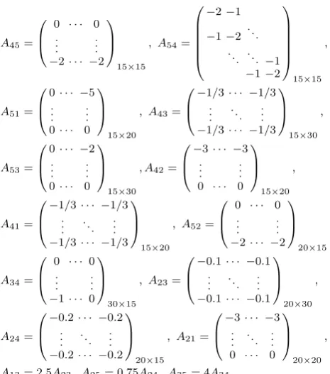
A45=



 

0 · · · 0

. . .

−2· · · −2



 

15×15

, A54=



     

−2−1

−1−2 . .. . ._. . ._. ₋₁

−1−2



     

15×15

,

A51=



 

0· · · −5

. . .

0· · · 0



 

15×20

, A43=



 

−1/3· · · −1/3

. .

. . .. ...

−1/3· · · −1/3



 

15×30

,

A53=



 

0· · · −2

. . .

0· · · 0



 

15×30

, A42=



 

−3· · · −3

. . .

0 · · · 0



 

15×20

,

A41=



 

−1/3· · · −1/3

. .

. . .. ...

−1/3· · · −1/3



 

15×20

, A52=



 

0 · · · 0

. . .

−2· · · −2



 

20×15

,

A34=



 

0 · · · 0

. . .

−1· · · 0



 

30×15

, A23=



 

−0.1· · · −0.1

. .

. . .. ...

−0.1· · · −0.1



 

20×30

,

A24=



 

−0.2· · · −0.2

. .

. . .. ...

−0.2· · · −0.2



 

20×15

, A21=



 

−3· · · −3

. . . . .. ...

0 · · · 0



 

20×20

,

A13= 2.5A23, A25= 0.75A24, A35= 4A34.

In the following, we choose α = {1,3} in the Schur complement A/α. Without loss of generality, we assume

k.k = k.k∞, α = 2 S r=1

αir, α

0 ₌ S3 t=1

αjt, i1 = 1, i2 = 3,

j1 = 2, j2 = 4, j3 = 5 and A/α = ( ˜A(αt, αt)). By

computation, A ∈ I−BSDs. According to Theorem 4.1,

any eigenvalues λofA/α satisfies

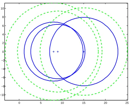
λ∈ {λ: |λ−15| ≤7.9186} ∪ {λ:|λ−8| ≤6.8310} ∪{λ:|λ−9| ≤6.2910}= Γ1.

By Theorem 3.13 in [20] and Theorem 3.5 in [21], any eigenvaluesλof A/αsatisfies

λ∈ {λ: |λ−15| ≤9.2727} ∪ {λ:|λ−8| ≤9.5455} ∪{λ:|λ−9| ≤8.1818}= Γ2.

By Theorem 3.1.1 in [35], any eigenvaluesλofA/αsatisfies

λ∈ {λ: |λ−15| ≤9.2424} ∪ {λ:|λ−8| ≤9.4697} ∪{λ:|λ−9| ≤8.1515}= Γ3.

By Theorem 4.1 in [13], any eigenvaluesλofA/αsatisfies

λ∈ {λ: |λ−15| ≤10.1250} ∪ {λ:|λ−8| ≤11.2500} ∪{λ:|λ−9| ≤9.3750}= Γ4.

To further confirm the facts in the above results, Figures 1-3 depict the eigenvalue distributions of the Schur complement. From these numerical results and figures, we have the following observations:

• As observed in the comparison results, the Theorem 3.13 in [20], Theorem 3.5 in [21], Theorem 3.1.1 in [35], Theorem 4.1 in [13] and Theorem 4.1 can suc-ceed in computing and determining the the eigenvalue distributions of the Schur complement by using the elements of the original matrix, whereas the eigenvalue distributions derived by Theorem 4.1 are sharper than

0 5 10 15 20

[image:10.595.54.287.68.332.2]

−10 −8 −6 −4 −2 0 2 4 6 8 10

Fig. 1. The blue solid line and the green dashed line denote the corresponding discsΓ1 andΓ2, respectively

0 5 10 15 20

−10 −8 −6 −4 −2 0 2 4 6 8 10

Fig. 2. The blue solid line and the green dashed line denote the corresponding discsΓ1 andΓ3, respectively

the ones computed by Theorem 3.13 in [20], Theorem 3.5 in [21], Theorem 3.1.1 in [35] and Theorem 4.1 in [13], that is,Γ1⊂Γ2,Γ1⊂Γ3andΓ1⊂Γ4.

• From Figures 1-3, we clearly find thatΓ1is the tightest among all eigenvalue distributions, which demonstrates the validity of the conclusion given in Remark 4.1. Example 6.2Let

A=

 

A11A12A13

A21A22A23

A31A32A33  ,

where

A11=

8 0 0 8

, A12=

0 1

, A13=

0 0 1 0

,

A21= 0 2

, A22= 10, A23= 3 0

,

A31=

0 3 0 0

, A32

1 0

, A33=

9 0 0 9

.

It is easy to see that A ∈ I−BSD3. We compare the bounds in Theorem 5.1 with those in Theorem 3.61 of [34]

IAENG International Journal of Applied Mathematics, 47:2, IJAM_47_2_07

[image:10.595.308.539.298.486.2]

(11)

0 5 10 15 20 25 −10

[image:11.595.52.282.60.249.2]

−8 −6 −4 −2 0 2 4 6 8 10

Fig. 3. The blue solid line and the green dashed line denote the corresponding discsΓ1andΓ4, respectively

and Theorem 3.2.3 of [35]. By utilizing Theorem 3.61 in [34], we have

35403≤ |detA| ≤70596.

By making use of Theorem 3.2.3 in [35], we have

43643≤ |detA| ≤60938.

Now, by applying Theorem 5.1, we derive

43841≤ |detA| ≤60703,

which is an improvement on the bounds in Theorem 3.61 of [34] and Theorem 3.2.3 of [35]. This example shows that the upper and lower bounds in Theorem 5 are better than those in Theorem 3.61 of [34] and Theorem 3.2.3 of [35]. In fact, detA= 47448.

VII. CONCLUSIONS

To estimates diagonally dominant degree on the Schur complement of matrices, we first exhibit some new esti-mations of diagonally dominant degree on the Schur com-plement of I(II)-block diagonally dominant matrices in this paper, which are proved to be sharper than the ones in [13], [35], [21]. As applications, some new distributions for the eigenvalues of the Schur complement of matrices as well as the new upper and lower bounds for determinants of the I(II)-block diagonally dominant matrices are derived, these results are better compared with those of [13], [35], [21], [34]. Numerical examples are also given to illustrate these facts.

It would be nice if we can find more precise estimates of I(II)-block diagonally dominant degree for Schur com-plement of matrices, distributions for the eigenvalues of the Schur complement of matrices and upper and lower bound-s for determinantbound-s of the I(II)-block diagonally dominant matrices compared those proposed in this paper. We will continue to research this topic in our further work.

REFERENCES

[1] D. Carlson and T. Markham, “Schur complements on diagonally dominant matrices,”Czechoslov. Math. J., vol. 29, no. 1, pp. 246–251, 1979.

[2] R. A. Horn and C. R. Johnson,Topics in Matrix Analysis. Cambridge University Press, 1991.

[3] K. D. Ikramov, “Invariance of the Brauer diagonal dominance in Gaussian elimination,”Vestn. Mosk. Univ., Ser. 15 Vyˇcisl. Mat. kibern, vol. 2, pp. 91–94, 1989.

[4] R. Smith, “Some interlacing properties of the Schur complement of a Hermitian matrix,”Linear Algebra Appl., vol. 177, pp. 137–144, 1992. [5] F.-Z. Zhang,The Schur Complement and Its Applications. Springer,

New York, 2005.

[6] J.-Z. Liu and Y.-Q. Huang, “The Schur complements of generalized doubly diagonally dominant matrices,”Linear Algebra Appl., vol. 378, pp. 231–244, 2004.

[7] J.-Z. Liu, Z.-J. Huang, and J. Zhang, “The dominant degree and disc theorem for the Schur complement,”Appl. Math. Comput., vol. 215, pp. 4055–4066, 2010.

[8] J.-Z. Liu and Z.-J. Huang, “The Schur complement ofγ-diagonally and productγ-diagonally dominant matrix and their disc seperation,”

Linear Algebra Appl., vol. 432, pp. 1090–1104, 2010.

[9] M.-Z. Zhu and Y.-E. Qi, “On the Eigenvalues Distribution of Precon-ditioned Block Two-by-two Matrix,”IAENG International Journal of Applied Mathematics, vol. 46, no. 4, pp. 500–504, 2016.

[10] Z.-G. Huang, L.-G. Wang, Z. Xu, and J.-J. Cui, “Convergence Analysis of Some New Preconditioned AOR Iterative Methods forL-matrices,”

IAENG International Journal of Applied Mathematics, vol. 46, no. 2, pp. 202–209, 2016.

[11] A.-J. Li, “Improving AOR Iterative Methods For Irreducible L-matrices,”Engineering Letters, vol. 19, no. 1, pp. 46–49, 2011. [12] J.-G. Hu, “The estimate of kM−1Nk∞ and the optimally scaled

matrix,”JCM Sinica, vol. 3, pp. 122–129, 1982.

[13] J.-Z. Liu, Z.-H. Huang, L. Zhu, and Z.-J. Huang, “Theorems on schur complement of block diagonally dominant matrices and their application in reducing the order for the solution of large scale linear systems,”Linear Algebra Appl., vol. 435, pp. 3085–3100, 2011. [14] J.-Z. Liu, J.-C. Li, and Z.-H. Huang, “Some properties on Schur

complement and diagonal Schur compelment of some diagonally dominant matrices,”Linear Algebra Appl., vol. 428, no. 1, pp. 1009– 1030, 2008.

[15] B. Li and M. Tsatsomeros, “Doubly diagonally dominant matrices,”

[16] J.-Z. Liu and Y.-Q. Huang, “Some properties on Schur complement of H-matrices and diagonally dominant matrices,”Linear Algebra Appl., vol. 389, pp. 365–380, 2004.

[17] J.-Z. Liu and F.-Z. Zhang, “Disc separation of the Schur complements of diagonally dominant matrices and determinantal bounds,”SIAM J. Matrix Anal. Appl., vol. 27, pp. 665–674, 2005.

[18] J. Zhang, J. Z. Liu, and G. Tu, “The improved disc theorems for the Schur complements of diagonally dominant matrices,”J. Inequal. Appl., vol. 2013, no. 2, 2013.

[19] Y.-T. Li and F. Wang, “The estimates of diagonally dominant degree and eigenvalues distributions for Schur complements of matrices,”J. Inequal. Appl., vol. 2013, no. 431, 2013.

[20] F. Wang, Criteria for H-matrices (tensors) and research of Schur complement of H-matrices (tensors). Yunnan University, Kunming, 2014.

[21] F. Wang and D.-S. Sun, “The estimates of diagonally dominant degree and eigenvalues inclusion regions for the Schur complement of block diagonally dominant matrices,” Open Math., vol. 13, pp. 781–794, 2015.

[22] R. Vein and P. Dale,Determinants and Their Applications in Mathe-matical Physics. Applied Mathematical Sciences, Springer, 1999. [23] M. I. Gil0_,_{Operator Functions and Localization of Spectra}_. _Lecture

Notes in Mathematics, Springer, Berlin, 2003.

[24] C. Krattenthaler, “Advanced determinant calculus: a complement,”

[25] T.-Z. Huang and X.-P. Liu, “Estimations for Certain Determinants,”

Comput. Math. Appl., vol. 2015, no. 50, pp. 1677–1684, 2005. [26] H.-B. Li, T.-Z. Huang, and H. Li, “Some New Results on

Determi-nantal Inequalities and Applications,”J. Inequal. Appl., vol. Article ID 847357, doi:10.1155/2010/847357, 2010.

[27] D. G. Feingold and R. S. Varga, “Block diagonally dominant matrices and generalizations of the gerschgorin circle theorem,”Pacific J. Math., vol. 12, no. 1, pp. 1241–1250, 1962.

[28] Z.-Y. You and Z.-Q. Jiang, “The diagonal dominance of block matri-ces,”J. Xian Jiaotong Univ., vol. 18, no. 3, pp. 123–125, 1984.

IAENG International Journal of Applied Mathematics, 47:2, IJAM_47_2_07

(12)

[29] S.-H. Xiang and Z.-Y. You, “Weak block diagonally dominant ma-trices, weak block h-matrix and their applications,”Linear Algebra Appl., vol. 282, pp. 263–274, 1998.

[30] C.-Y. Zhang, Y.-T. Li, and F. Chen, “On schur complement of block diagonally dominant matrices,”Linear Algebra Appl., vol. 414, pp. 533–546, 2006.

[31] B. Polman, “Incomplete blockwise factorizations of (block) H-matrices,”Linear Algebra Appl., vol. 90, pp. 119–132, 1987. [32] F. Robert, “Block H-matrices et convergence des methods iterations

classiques par blocks,”Linear Algebra Appl., vol. 6, pp. 223–265, 1969.

[33] L. Y. Kolotilina, “Nonsingularity/singularity criteria for nonstrictly block diagonally dominant matrices,”Linear Algebra Appl., vol. 359, pp. 133–159, 2003.

[34] L. Zhu, Properties, Criteria and Application for Block Diagonally Dominant Matrices. Xiangtan University, Xiangtan, 2007. [35] N.-N. Xu,The Block Dominant Degree and Disc Theorem on Schur

Complements of Block Diagonally Dominant matrices. Xiangtan University, Xiangtan, 2009.

[36] Z. Xu, Q. Lu, K. Y. Zhang, and X. H. An,Theory and Applications of H-matrices. Science Press, 2013.