warwick.ac.uk/lib-publications
A Thesis Submitted for the Degree of PhD at the University of Warwick
Permanent WRAP URL:
http://wrap.warwick.ac.uk/94093
Copyright and reuse:
This thesis is made available online and is protected by original copyright. Please scroll down to view the document itself.
Please refer to the repository record for this item for information to help you to cite it. Our policy information is available from the repository home page.
An Investigation into Methods
to aid the Simulation of Turbulent
Separation Control
by
Adam Preece
A thesis submitted in partial fulfilment of the requirements
for the degree of
Doctor of Philosophy in Engineering
Supervisors: Prof. Peter W. Carpenter
and Dr. Yongmann M. Chung
University of Warwick, School of Engineering
Fluid Dynamics Research Centre
In memory of
Professor Peter W. Carpenter
Contents
Contents
List of Figures
List of Tables
Acknowledgments
Declaration
Abstract
Abbreviations
Nomenclature
1 Introduction
1.1 The Political Climate . . . . 1.2 The Need for Computational Tools 1.3 The Scope & Content of this Work . i
v
xi
xiii
xiv
xv
xvi
xvii
xix
1
1 2
2 Literature Review
of Turbulent Separation Control 2.1 Turbulent boundary-layers
with zero pressure gradients 2.1.1 Turbulence . . . 2.1.2 The Velocity Profile.
2.1.3 Boundary-layer Development along a flat-plate. 2.2 Turbulent boundary-layers
in adverse pressure gradients. 2.2.1 Theory... 2.2.2 Experimental Studies . 2.2.3 The Lille Bump . . .. 2.2.4 Computational Studies 2.3 Separation control using steady jets
2.3.1 Previous Studies . . . . 2.3.2 Lille work on steady jets 2.4 Separation control using synthetic jets
2.4.1 Previous Studies . . . . 2.4.2 Lille work using Unsteady Jets. 2.5 Conclusions . . . .
3 Numerical Methods 43
3.1 Code Features . . 43
3.1.1 Discretization 44
3.1.2 Differencing Schemes 45
3.1.3 The TDMA Solver 50
3.1.4 The SIMPLE Algorithm 52
3.1.5 Turbulence Modelling. 56
3.1.6 Grid Generation. 56
3.2 Code Validation . 57
3.3 Conclusions
...
614 Immersed Boundary Methods 64
4.1 History. 65
4.2 Theory. 69
4.2.1 Solid Block Reconstruction . 70
4.2.2 Simple Linear Reconstruction 71
4.2.3 Full Linear Reconstruction 72
4.2.4 Quadratic Reconstruction 75
4.3 Applying the boundary conditions . 77
4.3.1 Pressure Treatment . . . 82
4.3.2 The Staggered Grid Formulation 83
4.4 Validation . . . 84
4.4.1 Steady Flow around a circular cylinder (ReD = 40) . . 4.4.2 Unsteady Flow around a circular cylinder (ReD = 100) 4.5 Conclusions . . . .
5 Turbulence Modelling using Wall Functions
5.1 The need for turbulence modelling. 5.2 Approaching turbulence treatment
5.2.1 Turbulence Modelling . . . .
5.3 The Spalart-Allmaras (S-A) Turbulence Model.
84 89 95 110 112 114 115 117
5.3.1 Practical & Numerical Aspects . 121
5.3.2 Validation of the basic S-A model 122
5.3.3 The effect of the inlet eddy viscosity boundary condition 131 5.3.4 The effect of the first off-wall node . . . 138 5.3.5 Conclusions to be drawn regarding the S-A model 140 5.4 Modifying the S-A Model using wall functions
5.4.1 Theory.. 5.4.2 Validation 5.5 Conclusions . . .
6 Detached Eddy Simulation
6.1 Validation of the DES Formulation 6.2 The Coarse Grid Results . . ..
6.3 The Fine Grid Results 6.4 Conclusions . . . .
7 Simulating Flow Control: A Feasibility Study
7.1 Setting up the Lille simulations . . . . 7.1.1 The Uncontrolled Case of Bernard et al. (2003) 7.1.2 Problem selection.
7.1.3 Selection of grids . , 7.1.4 Boundary Conditions.
7.1.5 Numerical Methods. 7.2 The uncontrolled case . . . .
7.2.1 The Simulation Parameters 7.2.2 The Effect of Grids
7.2.3 Comparison of the Methods 7.3 Simulating the steady jet case . . .
7.3.1 The Cross-stream Flow-field 7.3.2 The streamwise flow-field. 7.4 Conclusions . . . .
8 . Conclusions & Further Work
Bibliography v 172 178 179 181 181 182 184 185 186 187 187 189 192 . 207 . 209 220 228
230
List of
Figures
2.1 A typical turbulent velocity profile 36
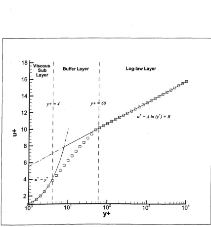
2.2 The Law of the Wall . . . 37
2.3 The effects of pressure on a small element of fluid 38 2.4 The 'bump' test section at the University of Lille 39 2.5 A schematic of the Lille bump set-up . . . 39 2.6 The uncontrolled pressure distribution over the Lille bump 41 2.7 Round steady-jet flow-control set-up of Godard and Stanislas (2006b) 41
3.1 Discretizing a simple one-dimensional system. 46
3.2 The Staggered Grid System . . . 58 3.3 The grid mesh chosen for the backward-facing step flow. 61 3.4 Stream-trace results for the backward-facing step flow. . 62 3.5 Comparison of recirculation lengths for backward-facing step flow 63
4.1 Modelling complex geometries . . 65
4.2 The Immersed Boundary Method 77
4.3 Simple Linear Reconstruction 78
4.4 Full Linear Reconstruction . . 79
4.5 Why the coefficients are negative 80
4.6 The behaviour of the coefficients . 80
4.7 Set-up for the circular cylinder validation simulations 92 4.8 Experimental Results of flow around a circular cylinder at ReD
=
41 . 934.9 Drag coefficients for a circular cylinder 93
4.10 The simulation grid set-up . . . 94
4.11 Streamtrace plots for different Immersed Boundary Methods 95 4.12 Pressure Distributionaround the cylinder at ReD
=
40 for the finest grid 96 4.13 Pressure Distribution around the cylinder at ReD=
40 for theintermediate-fine grid
...
974.14 Pressure Distribution around the cylinder at ReD = 40 for the intermediate-coarse grid . . . .. 98 4.15 Pressure Distribution around the cylinder at ReD
=
40 for the fine grid 99 4.16 Pressure Distribution around the cylinder at ReD = 40 for the solid-blockapproximation . . . " . . . 100 4.17 Pressure Distribution around the cylinder at ReD = 40 for the simple
linear method . . . 101 4.18 Pressure Distribution around the cylinder at ReD = 40 for the full linear
method
...
1024.19 Pressure Distribution around the cylinder at ReD
=
40 for the quadratic method . . . . . . . 1034.20 Grid sensitivity to drag coefficient .. . . . 104 4.21 Vorticity contours showing vortex shedding at Re = 100. 105 4.22 Strouhal numbers for given grid meshes and methods . . 106 4.23 Average drag coefficients for given grid meshes and methods 107 4.24 RMS lift coefficients for given grid meshes and methods. . . 108
5.1 Model Functions
Iv!
andIv2
from Spalart and Allmaras (1994) . 1205.2 Setup of S-A validation case 122
5.3 Velocity profile at x = 2.0m 124
5.4 Law of the wall profile at x = 108 125
5.5 Modified Turbulent Viscosity profile at x = 108 126
5.6 Displacement Thickness, 8* along the domain. 128
5.7 Momentum Thickness,
e
along the domain . 1295.8 Wall shear stress, Tw , along the domain. . 130
5.9 Figure 4 from Spalart and Allmaras (1994) 132
5.10 Inlet boundary conditions for modified eddy viscosity, j) • 134
5.11 Overall velocity profile at x=2.0m . . 135
5.12 Near-wall velocity profile at x=2.0m . 136
5.13 S-A Eddy Viscosity, j) at x=2.0m 137
5.14 Overall velocity profile at x=2.0m 141
5.15 Non-dimensional near-wall velocity profile at x=2.0m 142 5.16 The need for wall functions . . . 144
[image:11.513.64.485.190.760.2]5.17 Grid node position versus index . 5.18 Wall function results for Grid 01 . 5.19 Wall function results for Grid 02 . 5.20 Wall function results for Grid 03 . 5.21 Wall function results for Grid 04 . 5.22 Wall function results for Grid 05 . 5.23 Wall function results for Grid 06 . 5.24 Wall function results for Grid 07 . 5.25 Wall function results for Grid 08 .
5.26 First and second derivatives for a typical law of the wall profile. 5.27 Summary of wall functions results . . . .
6.1 Set-up of the backward facing step simulations.
148 152 153 154 155 156 157 158 159 160 161 165 6.2 Wall distance and maximum grid spacing for the coarse grid . 166 6.3 The Destruction Length Scale, d, distribution for the coarse grid. 167 6.4 Coarse grid for the backward facing step simulations . . . 168 6.5 The RANS and LES regions for the DES simulation using the coarse grid 169 6.6 Streamtraces for the coarse grid (a) RANS, (b) DES. . . 169 6.7 Modified turbulent viscosity, (i/) contours. . . 170 6.8 Instantaneous u-velocity contours for the coarse grid (a) RANS, (b) DES 171 6.9 Mean u-velocity contours for the coarse grid (a) RANS, (b) DES. . .. 172 6.10 Instantaneous vorticity contours for the coarse grid (a) RANS, (b) DES 173
6.11 Fine grid for the backward facing step simulations . . . .. 174 6.12 The RANS and LES regions for the DES simulation using the fine grid 175 6.13 Instantaneous Streamtraces for the fine grid (a) RANS, (b) DES. 175 6.14 Mean Streamtraces for the fine grid (a) RANS, (b) DES 176 6.15 Modified turbulent viscosity, (£I) contours. . . 177 6.16 Vorticity contours for the fine grid (a) RANS, (b) DES 177
7.1 Grid refinement study for the uncontrolled case (Cp ) 190
7.2 Grid refinement study for the uncontrolled case
('tw)
191 7.3 Streamtrace plots for the uncontrolled case (No IBM) 193 7.4 Streamtrace plots for the uncontrolled case (with IBM) . 194 7.5 Pressure coefficient distribution for the uncontrolled case 197 7.6 Velocity at the edge of the boundary layer for the uncontrolled case 198 7.7 Velocity profiles for the uncontrolled case. . . 199 7.8 Turbulent Viscosity profiles for the uncontrolled case 201 7.9 Displacement thickness for the uncontrolled case. 2027.10 Momentum thickness for the uncontrolled case. 203
7.11 Shape factor H for the uncontrolled case . . . . 204 7.12 Wall shear stress distribution for the uncontrolled case . 206 7.13 u-velocity contours at x = 0.5m downstream ofthe apex for the steady-jet
control case . . . 210
7.14 u-velocity contours at x = l.Om downstream ofthe apex for the steady-jet control case . . . 211 7.15 u-velocity contours at x = l.5m downstream of the apex for the steady-jet
control case . . . 212 7.16 Streamwise vorticity contours at x = 0.5m downstream of the apex for
the steady-jet control case . . . 213 7.17 Streamwise vorticity contours at x = l.Om downstream of the apex for
the steady-jet control case . . . 214 7.18 Streamwise vorticity contours at x = l.5m downstream of the apex for
the steady-jet control case . . . 215 7.19 Eddy-viscosity ratio contours (vt/v) at x = 0.5m downstream of the apex
for the steady-jet control case . . . 217 7.20 Eddy-viscosity ratio contours (vt/v) at x
=
l.Om downstream of the apexfor the steady-jet control case . . . 218 7.21 Eddy-viscosity ratio contours (vt/v) at x
=
l.5m downstream of the apexfor the steady-jet control case . . . 219 7.22 Spanwise averaged pressure coefficient for steady jet controlled case 221 7.23 Spanwise averaged edge velocity for steady jet controlled case . . . 222 7.24 Spanwise averaged edge displacement thickness for steady jet controlled
case . . . . 7.25 Spanwise averaged momentum thickness for steady jet controlled case 7.26 Spanwise averaged shape function H12 for steady jet controlled case
7.27 Spanwise averaged wall shear stress for steady jet controlled case ..
xi
List of Tables
2.1 Surface coordinates of the Lille Bump . . . ., 40 2.2 Parameters for the optimization study of the co-rotating jet system
de-tailed in Godard and Stanislas (2006b) . . . . . . . , 42 2.3 Parameters for the optimization study of the counter-rotating jet system
detailed in Godard and Stanislas (2006b) . . . ., 42
3.1 Parameters & Results for the case of the backward-facing-step
4.1 Grid Properties . . . . 4.2 Table of results for Re=40 for the finest grid spacing (D/20) 4.3 Table of results for Re=100 for the finest grid spacing (D/20)
. . .. 61
86 88 91
5.1 Constants for S-A turbulence model as given in Spalart and Allmaras (1994) . . . .
5.2 Boundary Layer Properties at x = 2.0m . . . . 5.3 Results at x = 108 when changing the inlet iI conditions 5.4 Grid Properties
5.5 Grid Properties
xii
7.1 Parameters for the uncontrolled Lille bump case (RSOl) . 188 7.2 Separation result$ for the uncontrolled Lille bump case 195 7.3 Forces and coefficients on the bump for the uncontrolled case. 207 7.4 Parameters for the steady-jet bump case (RS02) . . . 208 7.5 Forces and coefficients on the bump for the steady-jet case 228
Acknowledgments
Any acknowledgments must begin with special thanks for my supervisors Prof. Peter Carpenter & Dr. Yongmann Chung without whose help this work would not have even come close to completion. Sadly, Peter passed away before I managed to submit this work so for this reason, I have dedicated this thesis to his memory. Thankfully, Yongmann stepped in to supervise my work for the actual submission and, even though he was snowed under with marking, still managed to read every chapter and offer suggestions. Thanks must also go to Prof. Paul Tucker for his help as supervisor in my first year and his continuing advice in the development of his NEAT code.
I'd also like to thank everyone in the School of Engineering who's made this possible even just in allowing me to bounce my ideas off them! Gwilym & Novak for their help in getting my head around LaTeX & JabRef, Paddy for helping with my circular cylinder validation work & writing work, Mark E for general encouragement and Mark B for allowing me to clear up my own mind by discussing my work with someone else (as well as by climbing!). Thanks to Karen for help with formatting the thesis and the early morning chats over tea. And, of course, not to forget Juice for working together on im-plementing both the Immersed Boundary Methods and the turbulent inflow simulations.
Finally, but most importantly, I want to thank my family & friends without whose sup-port, I would have failed long go. Thanks must go to my parents for always believing I could do it, my fiancee Milla for providing a calm voice (and plenty of tea!) when I needed it and Wallace for providing a crazy distraction at the right times!
This research has been funded by the EPSRC and the European AEROMEMS II project.
Declaration
This thesis, and the material in it, is my own work. It has not been submitted for a degree at any other university.
As part of the work carried out, the following paper was published:
• Preece et al. (2004)
Abstract
The reduction of drag on commercial aircraft is an active field of study especially with environmental pressures to reduce the carbon emissions associated with climate change. To this end, the AEROMEMS-II project was commissioned by the EU with a view to investigate methods for reducing drag by using MEMS devices for controlling separation. One method for investigating flow control devices is to use the field of Computational Fluid Dynamics (CFD) to simulate the flow interactions produced in flow control appli-cations and assess their effect.
Simulating such flows can be computationally expensive so a number of methods have been investigated here to assess their use in flow control simulation applications. The first of these is the Immersed Boundary Method (IBM) which allows complex geometries to be simulated using simple cartesian grid CFD codes. IBMs are found to reduce requirements whilst maintaining flow resolution and accuracy.
Next is the use of turbulence modelling with wall functions to reduce the need for fine grids near any solid surfaces. This method is found to work well and can allow the grid spacing near the wall to be 100 times coarser than with no wall functions applied. Finally, Detached Eddy Simulation (DES) has been considered as a method for allowing unsteady flow control structures to be simulated without being damped by conventional turbulence modelling. Each of these methods is presented, implemented and validated against known flow cases to assess their abilities fully.
All three methods have then been applied together to a known experimental turbulent flow-control set-up at the University of Lille (fellow partners in the AEROMEMS-II project) in order to assess the feasibility of using all of these methods together to simulate flow control. All three of these methods are seen to work well together although not always with the same effect.
Abbreviations
• CD: Central Differencing A method for approximating flow gradients using nodes
either side of a desired node
• CFD: Computational Fluid Dynamics The use of numerical simulations solved
using computer hardware to simulate fl~id flows
• DES: Detached Eddy Simulation The use of turbulence modelling near walls and
LES away
• DNS: Direct Numerical Simulation The use of sufficiently fine grids to resolve all
significant length scales within a turbulent flow
• EASM: Explicit Algebraic Stress Model A turbulence model which approximates
the turbulent Reynolds stresses directly. Detailed in Gatski and Speziale (1993)
• HWA: Hot-Wire Anemometry Th~ use of the cooling characteristics of a small length of electrically conducting wire to estimate the velocity over the wire
• IBM: Immersed Boundary Method The use of body forces to produce surface
ge-ometries not coincident with the computational mesh
• ILES: Implicit Large Eddy Simulation An LES simulation without an SGS model
the sub-grid scale eddies being modelled by the natural numerical dissipation within
the code .
• LDA: Laser Doppler Anemometry An experimental method involving the use of
laser doppler methods to measure the velocity of particles added to the flow
• LES: Large Eddy Simulation The use of a fine grid to model the largest turbulent
eddies and a turbulence model to resolve the sub-grid scale turbulence
• PIV: Particle Image Velocimetry An experimental method involving taking rapid snapshots of flow-borne particles in order to estimate the velocity of the flow around
those particles
• RANS: Reynolds-Averaged Navier-Stokes (equation) Usually referring to the use of Reynolds-Averaging to simplify the Navier-Stokes equations in order to use
tur-bulence modelling
• S-A Model: Spalart-Allmaras model A one equation RANS turbulent model solving for a modified eddy-viscosity as detailed in Spalart and Allmaras (1994)
• SGS: Sub-Grid Scale Usually pertaining to a model used in LES to approximate the turbulent dynamics below the grid scale
• SJ: Synthetic Jet A jet flow produced by entrainment caused by an zero-net mass-flow oscillatory jet output
• URANS: Unsteady Reynolds-Averaged Navier-Stokes (equation) As for RANS but including the unsteady derivative
Nomenclature
General Variables
x y
z
u(x, y, z, t) v(x, y, z,
t)
w(x, y, z, t) U(x, y, z)V(x, y, z)
W(x,y,z)
u'(x, y, z, t) v'(x, y, z, t) w'(x, y, z, t)
Coordinate in the streamwise direction Coordinate in the wall-normal direction
Coordinate in the cross-stream direction (normal to both x & y) Unsteady velocity in the x direction
Unsteady velocity in the y direction Unsteady velocity in the z direction Time-averaged velocity in the x direction Time-averaged velocity in the y direction Time-averaged velocity in the
z
direction Fluctuating velocity in the x direction Fluctuating velocity in the y directionFluctuating velocity in the
z
directiont
TimeT Time averaging period
Physical Fluid Variables
jt Molecular viscosity 1/ Kinematic viscosity p Air density
Boundary Layer Properties
Uoo Freestream velocity
Ue Boundary layer edge velocity
0 Displacement thickness 8 Momentum thickness
0** Kinetic energy thickness
H Shape factor, 0*/8 HI Shape factor, 8/0**
H* Modified Shape factor as given in Eqn. 2.22
y+ Non-dimensional y-coordinate (in wall units) u+ Non-dimensional velocity (in wall units)
Ur Friction velocity
'Tw Wall shear stress
8 Momentum thickness 8 Momentum thickness Turbulence Variables
U,2 Streamwise normal Reynolds stress V,2 Wall-normal Reynolds stress
W,2 Cross-stream normal Reynolds stress
u'v' Reynolds shear stress . Flow Control Variables
a Skew angle of jet in Godard and Stanislas (2006a) f3 Pitch angle of jet in Godard and Stanislas (2006a) cI> Jet diameter in Godard and Stanislas (2006a)
L Distance between two jets of a system in Godard and Stanislas (2006a) ). Distance between adjacent systems in Godard and Stanislas (2006a)
V R Velocity ratio in Godard and Stanislas (2006a) Numerical Variables
Ox Size of grid cell in x-direction
oy
Size of grid cell in y-directionOz Size of grid cell in z-direction
ap Numerical coefficient for cell, P
aE Numerical coefficient for cell to the east of cell P (I.e. i
+
1) aw Numerical coefficient for cell to the west of cell P (I.e. i-I) aN Numerical coefficient for cell to the north of cell P (I.e. j+
1)as Numerical coefficient for cell to the south of cell P (I.e. j - 1)
ap Numerical coefficient for cell to the front of cell P (I.e. k
+
1)aB Numerical coefficient for cell to the back of cell P (I.e. k - 1) S¢> Source term for variable cjJ at cell P
Chapter
1
Introduction
1.1
The Political Climate
The impact of air travel on our environment is of the utmost importance in today's political climate. From demonstrations about a third runway at Heathrow to the still much debated impact of carbon emissions on the global climate, the use of commercial aircraft seems to attract controversy at every turn.
Added to this is the fact that the number of air passengers in the UK alone has exploded from 4 million in 1954 to 228 million in 2005. With no sign that these numbers will not continue to increase at a similar rate, the commercial aircraft manufacturers are under increasing pressure to make their aircraft more efficient, produce less emissions and all with less noise. One major area for increasing aircraft efficiency is to reduce the overall drag hence drag reduction is an active area of research.
In order to approach this problem of drag reduction, a number of research programs
1.2 The Need for Computational Tools 2
have been funded with the intention of investigating novel methods of drag reduction. In particular, the AEROMEMS and AEROMEMS-II projects funded by the European union have been involved with the use of small jets to control turbulent separation and reduce drag as reported in War sop (2005). The current work has been produced in conjunction with the AEROMEMS-II project.
1.2
The Need for Computational Tools
As computational resources have become more powerful and prolific, the use of com-putational tools has become an essential part of the research and development process. To this end, the development of computational methods to aid the simulation of flow structures has become a vital field of study.
Whilst computing power has increased greatly, the ability to model a fully turbu-lent flow over an aircraft's wing at high Reynolds numbers is still unfeasible within a reasonable time-frame as covered in Spalart (2000). For this reason, any computational method which improves accuracy or reduces computational effort is worth investigating.
With these factors in mind, the purpose of this thesis has been to examine a number of recent methods within the field of Computational Fluid Dynamics (CFD) and consider their possible application within the context of turbulent separation control.
1.3 The Scope & Content of this Work
1.3 The Scope f.1 Content of this Work 3
both experimental and computational studies of steady and unsteady jets being used to control turbulent separation and provides context for the following work.
Chapter 3 considers the computational methods and CFD code used in this work as these are key to the subsequent validations. In order to test the accuracy of the code, a number of base-line simulations were performed to test its performance.
The main body of work is contained in Chapters 4, 5 and 6 in which the com-putational methods are investigated. Each of these chapters presents the need for the method and also contains a brief history. The methods are then validated against some well-established cases.
These begin with Chapter 4 in which the Immersed Boundary Method (IBM) is .
presented and validated using the case of circular cylinder flow. Novel work in this area has been done in applying the IBM to a SIMPLE pressure-correction code and in doing so, a new implementation involving coefficients has been formulated.
Chapter 5 pres~nts the turbulence modelling used and investigates the use of wall
functions to improve the accuracy of such models on a coarse grid. A novel imple-mentation of the wall functions method is also presented allowing the method to work alongside the IBM. Testing of the wall functions method has been done using the case of a flat plate turbulent boundary layer.
Finally, Chapter 6 considers Detached Eddy Simulations and provides a qualitative investigation into their use for a backward-facing step flow.
1.3 The Scope f3 Content of this Work
such methods could work together.
Chapter
2
Literature Review
of Turbulent Separation Control
The content of this chapter presents some background theory in addition to a review of the relevant literature into the area of turbulent boundary-layer flow control in order to provide a setting for the work that follows. The chapter begins by examining turbulent boundary layer properties and the work that has been done to characterize them. Next, separated flows are considered with research into the boundary-layer characteristics under separation being presented. Finally, a review into the works on separation control using steady and unsteady jets is covered with emphasis being placed on the work done at the Laboratoire de Mecanique de Lille as part of the AEROMEMS-II project.
Literature relevant to specific methods covered later will be presented at the begin-ning of the relevant chapters. For example, research into immersed boundary methods is not presented here but at the beginning of Chapter 4.
2.1 Turbulent boundary-layers with zero pressure gradients
2.1
Turbulent boundary-layers
with zero pressure gradients
2.1.1
Turbulence
6
The boundary-layer manifests itself physically as a thin region of fluid in contact with any solid surface exposed to a flow. For typical aeronautical applications, this thickness is observed to be typically of the order of 0.001 - O.OlL where L is some characteristic length scale in the main flow direction e.g. the chord of a wing section. This is covered in some depth in Houghton and Carpenter (2003).
A major characteristic of turbulent boundary-layers is that they are inherently unsteady even when based on flows that are steady by nature. The velocity within a turbulent boundary-layer can be decomposed into a mean and fluctuating component such that:
u(t) = U
+
u'(t) (2.1)where u(t) is the instantaneous velocity, U is the mean velocity and u'(t) is the fluctuating velocity. The mean velocity, U is defined as:
liT
U = lim - u(t)dt
T ... oo T 0 (2.2)
2.1.2 The Velocity Profile 7
u'(t) = u(t) - U (2.3)
2.1.2
The Velocity Profile
This velocity profile is shown graphically in Figure 2.1. Part (a) of the figure shows the instantaneous unsteady velocity profile across a turbulent boundary-layer, part (b) shows the mean velocity profile and part (c) shows the fluctuating velocity profile. Although there are analytical solutions for the N avier-Stokes equations for some laminar boundary-layers, no such solutions exist for turbulent flow because of their complex, non-linear behaviour. However, the observations of Prandtl (1904) lead to the approximation ofthe mean velocity profile by an inverse power law. Hence, for a turbulent boundary-layer, the mean velocity, U, at some height, y, above the wall is given approximately by:
U
(y)
~
Uoo =
J
(2.4)where n is the power of the profile.
As one examines the flow closer to the wall it is clear that the turbulent fluctuations will eventually be damped out by the proximity of the solid wall. This leads to the assessment that the layer of the fluid directly in contact with the surface is dominated by viscous effects. For Newtonian fluids, this results in the velocity varying linearly close to the wall. As the fluid in contact with the wall remains fixed to the surface by viscosity, it is assumed that the velocity there is the same as the wall velocity (the 'no-slip condition').
2.1.2 The Velocity Profile 8
(2.5)
where u+ and y+ are the velocity and wall distance respectively in wall units and defined as:
(2.6)
(2.7)
where p is the fluid density and Ur is known as the friction velocity defined as:
(2.8)
'T w is the wall shear stress and is defined as:
'Tw
=
J1,(dU)
dy wall
(2.9)
The near-wall layer in which the velocity distribution is linear is known as the viscous sub-layer but only exists up to a distance of roughly y+ = 5 from the wall. Near the wall but well above the viscous sub-layer, the boundary-layer is unrestricted by the surface and so the turbulent stresses dominate over the viscous stresses. In this region, the velocity profile is found experimentally to follow a logarithmic relation such as:
2.1.3 Boundary-layer Development along a fiat-plate 9
A number of values for the constants A and B have been found but it is generally accepted that they take the approximate values of 2.54 and 5.56 respectively as covered in Houghton and Carpenter (2003). This region of fully-developed turbulent flow is known as the log-law region.
In between the viscous sub-layer and the log-law region there exists a layer in which both viscous and inertia effects have a similar magnitude. This region is known as the buffer layer and is presented as a blended region between the viscous sub-layer and log-law region profiles. These relationships are known collectively as the law of the wall and are given in Figure 2.2 below. The initial formulation of the Law of the Wall was derived from experiments on pipe flow with the above formulation being proposed by Ludwieg and Tillmann (1949). See Coles (1956) for more detail.
2.1.3 Boundary-layer Development along a flat-plate
It has been mentioned that the velocity profile itself remains largely unchanged in the streamwise direction although it will experience a growth in the wall normal direction as the retarding effect of the wall causes the boundary-layer thickness to grow. There is a problem, however, with the calculation of the boundary-layer thickness. There is no clearly defined edge to the layer as the velocity profile tends slowly towards the freestream velocity only fully reaching the freestream value at infinity. Therefore it is often more practical to assess other properties from the velocity profile which relate directly to the fluxes of certain properties through the boundary-layer profile.
2.1.3 Boundary-layer Development along a fiat-plate 10
of flow retardation as it approaches the wall) can be calculated. The displacement thickness can then be thought of as the height through which the surface would need to be moved in order to preserve the mass flux through the profile at that plane assuming that the boundary-layer profile is replaced with the edge velocity all of the way to the wall. This also means that the displacement thickness is a measure of the mass-flux lost as a result of the boundary layer being retarded by the wall.
The displacement thickness is usually denoted by 0* and defined by:
(2.11) where Ue is the velocity at the edge of the boundary layer.
If one considers a similar property but concerned with the momentum flux through the area (and hence measures the momentum lost in the boundary layer), another prop-erty known as the momentum thickness (denoted by 0) can be derived as:
(2.12) Likewise, a thickness quantifying the kinetic energy flux is denoted by 0** and defined as:
0** =
{'X'J
~
(1 _
(~)
2)
dy. Jo
Ue Ue(2.13)
2.1.3 Boundary-layer Development along a flat-plate 11
these momentum fluxes around the slice, an equation representing the development of the boundary-layer along the plate is presented. This is given as:
(2.14) where
Va
is any suction applied at the surface. This equation is known as the Karman momentum integral equation.In the case of no surface suction, the suction velocity
Va
will be zero. Also, if as-suming the case of zero pressure gradient, the edge velocity Ue will remain constant along the plate (and be equal to the freest ream velocity Uoo ). This simplifies the momentum integral equation to: ~(2.15) This simplified equation can be used along with empirical relations for drag co-efficient in order to produce a semi-empirical relationship for the development of the boundary-layer along the plate without any pressure gradient.
Manipulating Equation (2.15) and assuming the boundary layer follows the sev-enth power-law profile in Equation (2.4) with n = 1/7 gives a relation for the above thicknesses in terms of the boundary-layer thickness as given below:
6* = 0.1256
() = 0.09736
6** = 0.1756
2.1.3 Boundary-layer Development along a flat-plate 12
Further information regarding this derivation can be found in Houghton and Car-penter (2003). Although providing information about the properties of a boundary-layer velocity profile in their own right, the integral thicknesses can also be combined to pro-vide further quantification of the boundary-layer. For example, one aspect that the displacement thickness does not reveal is whether the boundary-layer is 'biased' more towards the wall (as in a turbulent profile) or further away from the wall (as in a lam-inar profile) By calculating a ratio between two integral thicknesses, a shape factor, H is defined as:
8*
H=-() (2.17)
This shape factor is constant providing the velocity profile is not being acted upon by a pressure gradient or surface suction. For laminar boundary-layers, the shape factor is given in pages 412-414 of Houghton and Carpenter (2003) as approximately:
H~2.7 (2.18)
However, for a turbulent boundary-layer, using the power-law approximation, gives the shape factor as roughly:
0.1258
H = 0.09738
~
1.28 (2.19)2.1.3 Boundary-layer Development along a flat-plate 13
as the amount of momentum through the boundary-layer increases for a given displace-ment thickness (as is the case for a turbulent boundary-layer) then the shape factor reduces. This makes the shape factor useful in assessing the state of the boundary-layer. For example, the shape factor starting to increase, may be an indication that the boundary-layer may be starting to re-Iaminarise or may be under an adverse pressure gradient.
2.2 Turbulent boundary-layers in adverse pressure gradients
2.2
Turbulent boundary-layers
in adverse pressure gradients
14
Although the previous section examined the behaviour of turbulent boundary-layers without the effect of streamwise pressure gradients, this case is clearly a special one. All aerodynamic flows of engineering significance have some form of pressure distribution around them, so . leading to pressure gradients acting on the boundary-layers in the immediate vicinity of such objects.
A classic example of this is an aerofoil. The air approaches the aerofoil and slows down as it approaches the stagnation point on the leading edge. The air then splits around the aerofoil section and is forced to speed up in order to preserve continuity. This in turn causes the pressure to decrease along the surface in response. Past the thickest point of the aerofoil, the flow decelerates towards the freest ream velocity as it approaches the trailing edge, so causing the press~re to again rise to balance this. It can be seen from this example that generally, up to the point of maximum thickness, the pressure is dropping so producing a negative pressure gradient. Likewise, towards the trailing edge, the pressure is increasing so giving rise to a positive pressure gradient. A brief summary of the effect of these pressure gradients on the flow within the boundary-layer will now be given.
2.2.1
Theory
2.2.1 Theory 15
slow down the element as it travels through the boundary-layer. This gives rise to the boundary-layer development in the stream-wise direction as detailed above.
For turbulent boundary-layers these shear stresses are more complex than for lam-inar boundary-layers in that the fluctuating velocities produce turbulent stresses which vary with time. By following the Reynolds averaging process (see Chapter 5), these tur-bulent stresses, unchanging with respect to time, are many times larger in magnitude than the laminar shear stresses. This is the effect that causes a turbulent boundary-layer to grow more quickly than its laminar counterpart as shown in Houghton and Carpenter (2003) .
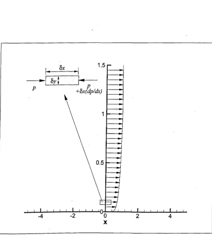
. However, the force which has the most effect when considering boundary-layer separation is the pressure gradient across the element. If the pressure on the left-hand face is given by p then the total pressure force on the element will be given by the following relation:
which simplifies to:
ap
Fp = --8x8y
ax
(2.20)
(2.21)
where Fp is the pressure force positive in the x direction. It is clear, therefore, that the pressure force on an element in a boundary layer is acted upon by a force directly proportional with the pressure gradient at that point.
2.2.1 Theory 16
To avoid confusion, a negative pressure gradient is known as a favourable pressure gra-dient to denote the effect it has on the boundary-layer. Conversely, a positive pressure gradient is known as an adverse pressure gradient as it acts against the boundary-layer. (However, one could argue that if one was trying to achieve separation, a positive pres-sure gradient should be known as favourable!)
The phenomenon of separation is known to occur when the pressure gradient is excessively adverse over a sufficient distance. This can be explained by considering the fluid 'layers' across a boundary-layer profile as it travels downstream. At the start of the adverse-pressure-gradient region, the profile would probably look very similar to the velocity profiles detailed in the previous section. As the profile convects downstream, all of the layers across the profile are retarded by the pressure gradient.
Unfortunately, the layers closest to the wall will have less momentum to begin with than the layers towards the edge of the boundary-layer as they are closest to the retarding effect of the wall. This means that at some point downstream, the velocity gradient at the wall (and hence the wall shear stress) will become zero. This point on the surface is known as the separation point and downstream of this point, the flow near the wall will begin to flow back upstream. If a streamline is drawn from the separation point and following the point on the profile at which the boundary-layer above has an equal mass flow to the boundary-layer before separation, then the fluid flow near the wall becomes separated into two regions. The region closest to the wall is now a recirculating region of fluid known as the separation region. Above this and below the freest ream flow, the boundary layer still exists but is said to be separated from the wall.
2.2.2 Experimental Studies 17
what criterion can be used to quantify separated flows, what effects separation has on a turbulent boundary-layer and how it can be better predicted. It is the use of computa-tional methods in order to predict separation and simulate separation-control methods that is the main aim of this present ~ork.
In order to better understand the physical behaviour of separation on turbulent boundary-layers, a summary of the experimental studies into this area will now be covered.
2.2.2 Experimental Studies
Although the previous section details in qualitative terms the effects of the pressure gradient on a typical boundary-layer, a review of the experimental studies done in this area is necessary to begin quantifying the problem.
In any flow experiencing a pressure gradient, there are a number of regions within the flow domain. To begin with, there is always a 'development region'. This is where the boundary-layer develops along a solid surface. With no pressure gradient present, the boundary-layer will develop as considered in the previous section. However, if a non-zero pressure gradient exists the boundary-layer will be different to the general case.
boundary-2.2.2 Experimental Studies 18
layer is actually less likely to separate under a favourable pressure gradient than under no pressure gradient at all. For this reason, the case of a favourable pressure gradient will not be examined.
The adverse pressure gradient, on the other hand, causes more complex effects. Until the point of separation, the velocity profile becomes retarded by the pressure gradient thus becoming less full with the near-wall velocity being retarded mostly due to it being further from the mainstream flow. This can be seen in many experimental works especially Spalart and Watmuff (1993), Dengel and Fernholz (1990) and Alving and Fernholz (1996).
Although the overall boundary-layer profile changes shape dramatically when plot-ted using conventional coordinates, the near-wall velocity profiles are observed to main-tain the law-of-the-wall behaviour detailed previously. As the wall shear stress is de-creasing more rapidly due to the pressure gradient, until the point of separation, (where T w
=
0 and hence y+=
0 & u+=
00) the dimensionless near-wall behaviour ismain-tained as shown in Samuel and Joubert (1974). However, because they do not cover the viscous sub-layer region due to measurement resolution it can be safely assumed that if the profile immediately above the buffer layer follows a good logarithmic behaviour then the viscous sub-layer is likely to be accurately followed.
2.2.2 Experimental Studies 19
an increase the displacement thickness at a faster rate than the increase in momentum thickness. The work by Dengel and Fernholz (1990) observed this behaviour in their work.
The retardation of the boundary-layer also has the effect of causing the wall shear stress to drop at a quicker rate as the velocity gradient at the wall decreases. As mentioned previously, once the wall shear stress has fallen to zero, the boundary-layer separates as the negative wall shear stress downstream of this point denotes a region of recirculating flow forcing the boundary-layer to leave the surface. This increased drop in wall shea~ stress can be illustrated by the work of Samuel and Joubert (1974). Their results show various boundary-layer properties from the positions x = 1.04m to x = 3.39m. This streamwise distance equates to the Reynolds number based on x increasing by a factor of 3.26. Over this distance, the drag coefficient is observed to decrease from 2.75 x 10⁻³ to 0.68 X 10⁻³ thus decreasing by a factor of roughly 4.
As the drag coefficient of a boundary-layer without a pressure gradient varies by the inverse of the fifth root of the Reynolds number, this gives the drag coefficient as decreasing by a factor of 1.27. This can be seen in Houghton and Carpenter (2003). This is around a third of the rate at which the adverse pressure gradient results decrease. Therefore, just for the example of the work by Samuel and Joubert (1974) it is not uncommon to see the drag coefficient decrease 5-10 times quicker in a moderate adverse pressure gradient.
2.2.2 Experimental Studies 20
for considering the flow, behaviour at the exact point of separation is that by Dengel and Fernholz (1990). Here an adverse pressure gradient is applied to the boundary-layer and carefully varied to cause the approach and onset of separation. The skin friction was measured by Preston tubes in the upstream portion of the flow whilst pulsed-wire probes were used where separation was observed.
An important point to note is that like most other properties of the turbulent boundary-layer, the separation point is unsteady with respect to time. In quantifying separation, an upstream-flow parameter is often employed providing a estimate of the fraction of time in which the flow is spent travelling back upstream. If this parameter equals 1.0, the flow is always travelling back upstream, if it is 0.0, the flow is always downstream and if it is 0.5, the flow spends an equal amount of time flowing upstream and downstream.
This upstream-flow parameter is also found to vary strongly with distance from the wall. Dengel and Fernholz (1990) show that the intermittency increases exponentially as one approaches the wall. This has the problem that it makes an estimate of an exact value for intermittency at the wall difficult to estimate by extrapolation. However, it was observed by Simpson et al. (1981) that the point of maximum intermittency does not lie at the wall but simply very close to it. They observed that the maximum point was at roughly
y/o
=
0.01 whilst Dengel and Fernholz (1990) did not have any readings below around 4mm which for a boundary-layer thickness of roughly 80mm only equates toy/o
~ 0.05.2.2.3 The Lille Bump 21
Fernholz (1990), Alving and Fernholz (1996) and Song et al. (2006) and consider the separation of flow through a two-dimensional geometry. The three Reynolds stresses present in a two-dimensional geometry consist of the streamwise normal Reynolds stress,
U,2, the wall normal Reynolds stress, V,2 and the Reynolds shear stress, u'v'
It is observed in Song et al. (2006) that as soon as the flow begins to separate, the peak in the streamwise normal Reynolds stress, U'2 moves from being very close
to the wall and starts to move away from the wall. The magnitude of this peak also begins to grow. Moving downstream, the peak grows in magnitude and moves further away from the wall. Eventually, the peak begins to diffuse into the overall boundary-layer distribution for U,2 as the layer begins to reattach itself. Similar behaviour is also
observed for the other Reynolds stresses V,2 and u'v'.
Of particular interest to the current work is the research done at the University of Lille into the effects of an adverse pressure gradient on a turbulent boundary layer and this will now be covered.
2.2.3 The Lille Bump
2.2.3 The Lille Bump 22
2.1 gives coordinates for the bump geometry.
Over recent years, a number of studies have been published by t'he team at Lille as work has progressed. The first work relevant to the current study can be found in Bernard et al. (2003). Here the velocity details of the flow are given by using hot-wire anemometry and the pressure at the surface of the bump is given by micromanometer transducers.
The bump starts at 15.5m from the beginning of the wind-tunnel base plate and ends at 19m. The wind tunnel cross section is 1 x 2m2• The maximum velocity through
the tunnel is lOms-1 so allowing Reynolds numbers (based on momentum thickness) of
2 x 10⁴ to be reached. There is little pressure gradient in the 15m run-up section of the tunnel with a value of -0.53Pa/m at lOms-1 being recorded.
The shape of the bump was computed by Dassault Aviation using k - c modelling in order to bring the flow behind the bump to the point of separation without actually separating. This was done to avoid any three-dimensional perturbations associated with separated flow and so allow the effects of various flow control devices to be more accurately analysed. As mentioned previously, the coordinates of the bump are given in Table 2.1.
The flow over the bump was run with the pressure and velocity profiles being recorded for later analysis. From these data a number of parameters were calculated. Firstly the external velocity at the edge of the boundary-layer increases to a maximum over the bump before reducing to the freestream value given at the inlet. This is to be expected as the flow speeds up to conserve mass over the bump.
2.2.4 Computational Studies 23
the boundary-layer was to separation. The modified shape factor was used as given in Schlichting (1979) as:
H*
=
0.5442HIJ
HIHI - 0.5049 (2.22)
where HI is the shape factor () / 8**.
Over the rear of the bump, a minimum shape factor, H* of 0.85 was found. As it is proposed that a modified shape factor of less than 0.761 indicates the boundary-layer is prone to separation, it is clear that the bump boundary-layer is close to separation.
The pressure distribution over the bump was found to follow the relationship shown in Figure 2.6. There is good agreement between the measured results from the pressure transducers and the computed results carried out by Dassault Aviation. It is clear that the pressure drops to a minimum over the apex of the hump where the velocity has increased to a maximum. As the flow reduces speed over the rear of the bump, the pressure rises again so placing the boundary-layer in this rear region under an adverse pressure gradient. This research is covered in greater depth later in Chapter 7 when it is compared with the simulations of the current work.
2.2.4 Computational Studies
2.2.4 Computational Studies
24
relies on fine grid resolution to model any turbulent structures. This resulted in the Reynolds number based on momentum thickness being around 600.
The recent NASA-CFDVAL2004 validation conference on synthetic jets and tur-bulent separation control held at the Langley Research Centre provided an excellent opportunity to compare various computational methods and approximations on identi-cal cases. This conference is of special significance to the present work as the author completed some synthetic jet simulations that were included in the proceedings.
The conference consisted of three cases with one of these involving the modelling of flow over a hump with a synthetic jet being applied for the purpose of flow control. Most of the works from this case were published recently in the AIAA Journal and are detailed in Rumsey et al. (2006). Only the uncontrolled separation cases will be considered in this section with the controlled case being considered later in Section 2.4.
The case set-up was based on the work by Seifert and Pack (2002) which employed a Glauert-Goldschmied type body, that is an aerofoil with a convex leading portion and a concave trailing portion. The model is 584mm wide, 53.7mm high and the length of the hump from the front to the back is 420mm. The Reynolds number based on chord length was Re = 9.29 x 10⁵ which equates to a Mach number of O.l.
In total, there were 13 contributors who ran 56 separate cases for the conference. The simulations were run mainly using RANS /URANS although a few did use blended RANS-LES results and even DNS. Grids were supplied by the conference organisers to avoid issues of grid resolution between submissions. The supplied structured and unstructured grids all had somewhere in the region of 50,000-250,000 nodes.
2.2.4 Computational Studies 25
wind-tunnel set-up. The location of the separation point was well calculated by all submissions which indicates that the turbulence models are well adjusted to calculate the point of zero wall shear stress. However, the reattachment length is less accurately predicted (roughly 10-20% too long) This could be as a result of under-prediction in the turbulent shear stress in the separated region where most submissions only predicted the magnitude as around 25% of the actual experimental measurements. This lack of turbulent shear stress would probably slow down the turbulent mixing from the outer regions of the boundary-layer down towards the wall so delaying reattachment.
Another issue that may affect the accuracy of a separation simulation is the order of the turbulence model being used. For example, the work of Morgan et al. (2006)
focussed on using High Order RANS (HO-RANS) k - c modelling to model flow over the flow-control case geometry. On initial inspection, simulations showed that using a second-order k - E model limited the overall simulation to second-order even if the base
code used a sixth order method. The HO-RANS method therefore allows the base code to achieve higher accuracy compared to the second-order method.
However, it should be noted that the biggest contribution made by this work was found during grid-refinement studies. It was shown that the HO-RANS simulations provided similar results to the lower-order model using a grid four times larger. This suggests that whilst the validity of RANS modelling for the highly unsteady flows en-countered in flow-separation control systems is debatable, the use of HO-RANS will inevitably provide a significant saving in computational resources as compared with the more standard second-order method.
2.2.4 Computational Studies 26
observed in turbulent boundary layers, the correlation between the various fluctuations will still be zero. This is because, if u' and v' vary independently, the correlation u'v'
(and hence the turbulent shear stress) will be zero.
One work which emphasises this point is that of Persson et al. (2005) and Persson
et al. (2006). It was observed for the DES simulations that the estimated level of turbulent viscosity at the inlet had a significant effect on the downstream flow. Similarly, it was also observed that varying the development length before the hump also had significant effect. To quote Persson et al. (2005):
For the DES calculations, improved agreement with the experimental data
was also obtained for the long inflow section suggesting that the resolvable
structures in the boundary-layer are not negligible.
This sensitivity of the downstream simulation to the inlet eddy viscosity was also experienced in the current work and is covered later in Chapter 5.
2.3 Separation control using steady jets
27
2.3
Separation control using steady jets
One way of controlling separation is to introduce momentum into the flow so making the boundary layer less prone to separation. This can be done in a variety of ways but one efficient way to achieve this is to introduce streamwise vorticity which has the effect of bringing higher momentum flow from the edge of the boundary layer down towards the wall.
2.3.1
Previous Studies
Much of the work in the area of steady jet separation control has been done by James Johnston of Stanford University. His research has been concerned with the use of pitched & skewed jets to induce streamwise vorticity in order to control turbulent separation. Key works include Johnston and Nishi (1990), Compton and Johnston (1992), Johnston (1999) and Johnston et al. (2002).
The best of these works that explain the general principles of pitched & skewed jets is given in Johnston and Nishi (1990). This consists of an experimental study using a wind tunnel with a variable upper surface to allow varying pressure gradients to be applied. The boundary-layer in question develops along a flat plate and proceeds past a trip in order to ensure turbulence. An array of variable geometry jets is placed a suitable distance downstream. These consist of circular holes in the lower surface of the tunnel which allow a plug to be fitted having a hole drilled through at the desired pitch angle of the jet (in this case 45 degrees). The skew angle can then be adjusted by rotating the 'plug' in the jet hole.
2.3.1 Previous Studies 28
combinations of jets paired together).
The resulting vortices were shown to produce peaks in the drag coefficient (and hence wall shear stress) directly under the vortices as a result of the sideways motion being imparted on the flow underneath the vortex. Between two counter-rotating vor-tices there seems to be either an increase or decrease in wall shear stress depending on whether the flow is being forced down or up between the vortices. However, on average, the wall shear stress is increased by the presence of the vortices. This is confirmed by the mean velocity profile downstream of the jets as shown in Johnston and Nishi (1990). The jet results in an increase of the velocity profile at the wall but does result in a reduced velocity profile at the edge of the boundary-layer. This shows the transfer of momentum from the outer part of the layer to the near-wall region which is of interest for separation control.
Compton and Johnston (1992) continues this work and looks to visualise the results using a five-hole pressure probe. The resulting visualisations, including vector and vorticity plots, show that the proposals of Johnston and Nishi (1990) were well founded. The vortices produced by the pitched & skewed jets are shown to travel and grow downstream so bringing the outer flow nearer the wall.
2.3.2 Lille work on steady jets 29
2.3.2
Lille work on steady jets
Godard and Stanislas (2006b) considers the application of fully round steady jets and their effects on the boundary layer. This work was similar in nature to the earlier works of Johnston and Nishi (1990) and Compton and Johnston (1992) although the focus is to measure the change in wall shear stress due to the induced vortices. The optimization study varied the following parameters; the skew angle of the jet, a, the pitch angle of the jet,
/3,
the jet diameter, if!/o, the spanwise distance between two jets of a system, L/if!, the spanwise distance between each system, A/if! and the velocity ratio, V R. A diagram of the set-up is given in Figure 2.7.Considering first the co-rotating system, the round jets appear to work reasonably well at low velocity ratio (around 1.6). Obviously as the velocity ratio is increased, the performance of the jets increases although in the co-rotating case, the velocity also varies the migration of the vortices in the spanwise direction. The skew angle of the jets makes little difference between 45 and 90 degrees confirming the previous work of Compton and Johnston (1992), although a value of 60 degrees seemed to give the best efficiency.
As with the slotted jets, decreasing the distance between the jets improves the performance, most likely because the vortices are working better together and less in isolation. Increasing the number of jets has the effect of reducing the spanwise variation of the peak wall shear stress although this does not result in an overall increase in performance.
2.3.2 Lille work on steady jets 30
2.4 Separation control using synthetic jets 31
2.4 Separation control using synthetic jets
2.4.1 Previous Studies
An unsteady jet is simply defined as a jet whose velocity characteristics vary with respect to time. They can be classified in a number of ways and, indeed, this sometimes leads to confusion as to which jet is being used. For the purpose of this work, two main groups of unsteady jets are considered. The first main group considers all jets which only expel air periodically but without any suction phase at all. These will be known as 'pulsed jets'. The other group considers all jets which have a suction phase equal in magnitude to the expulsion phase so imparting no net mass-flux to the flow. These are to be known as 'synthetic jets' but are also known in the literature as 'zero-net-mass-flux jets'.
In short, these jets work by the principle of generating a vortex pair or ring from the jet orifice as the flow is expelled from the jet. As the flow starts to reverse and flow back into the jet on the suction stroke, these vortices continue to travel away from the jet if the original momentum imparted by the synthetic jet is sufficient. If the average flow field is recorded a net mass-flux away from the jet is evident as a result of the vortex streaming.
The finer principles of synthetic jets are a complete field of study within itself and so will not be covered in greater depth here. However, some research has been done in this area for the current work as part of the NASA-CFDVAL conference and this has been published in Preece et al. (2004) and later in Rumsey et al. (2006). In addition, there is the excellent review on synthetic jets given in Glezer and Amitay (2002).