Parameter estimation and model fitting of stochastic processes

(1)

University of Warwick institutional repository: http://go.warwick.ac.uk/wrap

A Thesis Submitted for the Degree of PhD at the University of Warwick

http://go.warwick.ac.uk/wrap/51576

This thesis is made available online and is protected by original copyright.

Please scroll down to view the document itself.

(2)

Parameter Estimation and Model Fitting

of

Stochastic Processes

by

Fan Zhang

Thesis

Submitted to the University of Warwick in partial fulfillment of the requirements

for admission to the degree of

Doctor of Philosophy

(3)

Acknowledgments

Foremost, I would like to express my deepest gratitude to my supervisors, Professor Andrew Stuart and Doctor Anastasia Papavasiliou, for their continuous support through my PhD study, research and professional development, for the motivation, guidance, patience and knowledge they have provided through my PhD study. This thesis can not have been made possible without their guidance and tutorship. So, here again, I express my most sincere gratitude to their assistance.

I would also like to thank the members of the Applied Maths and Statistics seminar group and research fellows for their fruitful thoughts, critical but constructive comments and advices, assistance and help, especially Konstantinos Zygalakis, Simon Cotter, Yvo Pokern, Jochen Voss and David White.

I am also thankful to the financial support provided by the University Warwick Vice-Chancellor’s studentship, and the internship opportunity provided by International Mone-tary Fund to practice my learnings.

(7)

Declarations

(8)

Abstract

Multiscale methods such as averaging and homogenization have become an in-creasingly interesting topic in stochastic time series modelling. When applying the av-eraged/homogenized processes to applications such as parameter estimation and filtering problems, the resulting asymptotic properties are often weak. In this thesis, we focus on the above mentioned multiscale methods applied on Ornstein-Uhlenbeck processes. We find that the maximum likelihood based estimators for the drift and diffusion parameters derived from the averaged/homogenized systems can use the corresponding marginal mul-tiscale data as observations, and still provide a strong convergence to the true value as if the observations are from the averaged/homogenized systems themselves. The asymp-totic distribution for the estimators are studied in this thesis for the averaging problem, while that of the homogenization problem exhibit more difficulties and will be an interest of future work. In the case when applying the multiscale methods to the Kalman filter of Ornstein-Uhlenbeck systems, we study the convergence between the marginal covariance and marginal mean of the full scale system and those of the averaged/homogenized systems, by measuring their discrepancies.

(9)

List of Figures

3.1 Averaging: Consistency of Estimatorˆaǫ_T . . . 28

3.2 Averaging: Asymptotic Normality ofaˆǫ_T . . . 29

3.3 Averaging: Consistency ofqˆǫ δ . . . 30

3.4 Averaging: Asymptotic Normality ofqˆǫ_δ . . . 30

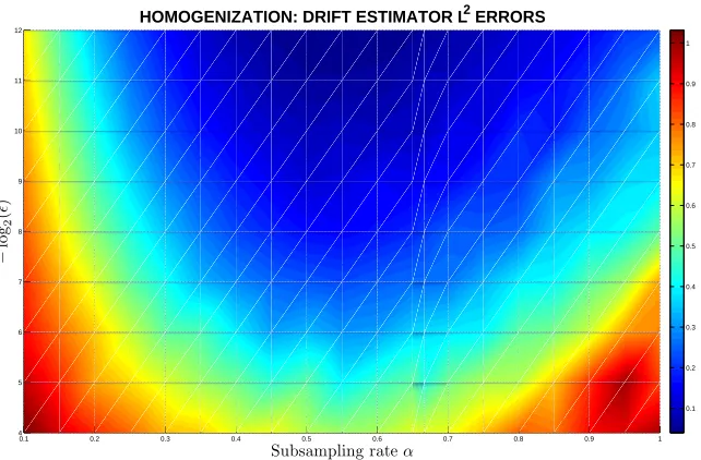
4.1 Homogenization: L2_{norm of}_(ˆ_a N,ǫ−˜a)for differentǫandα. . . 54

4.2 Homogenization: L2 norm of(ˆaN,ǫ−˜a)for different ǫand α(alternative view) . . . 54

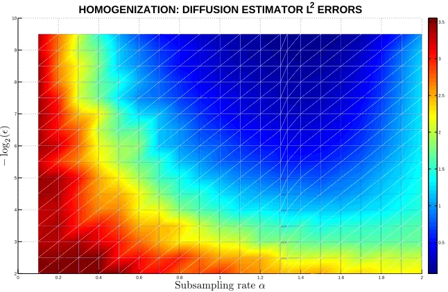
4.3 Homogenization: L2_{norm of}_(ˆ_q ǫ−q˜)for differentǫandα . . . 55

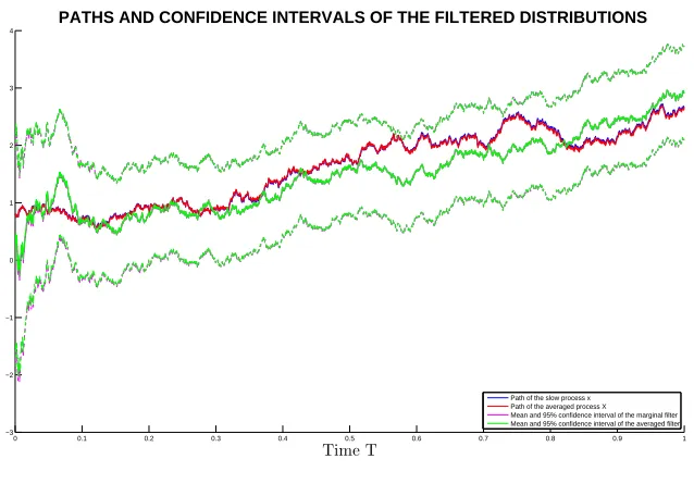
4.4 Homogenization: L2norm of(ˆqǫ−q˜)for differentǫandα(alternative view) 55 5.1 Paths and 95% confidence intervals of the filtered distributions . . . 69

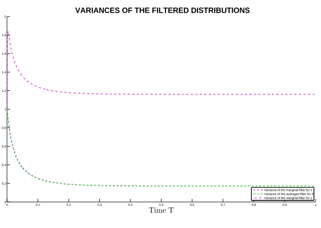
5.2 Variances of the filtered distributions . . . 70

5.3 Squared error between the means of the marginal and averaged filtered dis-tributions . . . 70

5.4 Error between the variances of the marginal and averaged filtered distributions 71 6.1 Paths and 95% confidence intervals of the filtered distributions . . . 86

6.2 Variances of the filtered distributions . . . 86

6.3 Squared error between the means of the marginal and homogenized filtered distributions . . . 87

6.4 Error between the variances of the marginal and homogenized filtered dis-tributions . . . 87

7.1 Autocorrelation Diagnostics for Model 3 . . . 101

7.2 Autocorrelation Diagnostics for Model 4 . . . 102

7.3 Raftery & Lewis test for Model 3 . . . 102

7.4 Raftery & Lewis test for Model 4 . . . 102

(10)

7.6 Geweke diagnostics for Model 4 . . . 105

7.7 Historical values of the Nelson-Siegel Parameters . . . 108

7.8 VAR(1) simulated Nelson-Siegel factors and Yield Curves . . . 109

7.9 Standard BVAR(1) simulated Nelson-Siegel factors and Yield Curves . . . 110

7.10 Simulated Nelson-Siegel factors and Yield Curves using Gibbs Sampled BVAR(1) . . . 111

7.11 Simulated Nelson-Siegel factors and Yield Curves using Heteroscedastic Regression model with Gibbs Sampler . . . 112

7.12 Historical Correlations . . . 113

7.13 Simulated Correlations based on VAR(1) . . . 114

7.14 Simulated Correlations based on standard BVAR(1) . . . 115

7.15 Simulated Correlations based on BVAR(1) with Gibbs Sampler . . . 116

7.16 Simulated Correlations based on Heteroscedastic Regression Model with Gibbs Sampler . . . 117

8.1 Historical correlation matrix of returns . . . 126

8.2 Simulated correlation matrix using CC-GARCH(1,1) . . . 127

8.3 Historical price index of all assets . . . 129

8.4 Historical log returns . . . 130

8.5 Autocorrelation function of historical returns . . . 131

8.6 Price index simulated using CC-GARCH . . . 132

8.7 Returns simulated using CC-GARCH . . . 133

8.8 Price index simulated using DCC-GARCH . . . 134

8.9 Returns simulated using DCC-GARCH . . . 135

(11)

Chapter 1

Introduction

The problem of parameter estimation for autoregressive (AR) type time series has long been a very popular topic. A large amount of literature focuses on parameter estimation problems for AR type models under different setups. In this thesis, we present parameter estimation strategies of AR type models within the framework of Ornstein Uhlenbeck stochastic dif-ferential equations in Part I and II, where the data are provided continuously, except when discretization is necessary. We present the problem within the Bayesian framework in Part III, where the data are provided discretely since it is based on real world applications.

Parameter estimation forms an essential part of the statistical inference methodolo-gies, especially for standard models such as Ornstein Uhlenbeck processes. In recent liter-atures, such as [1, 2, 69, 72], model fitting of multiscale data has become a popular topic in this area, since the finite dimensional data with different scales often become inconsistent with model at small scales when applying standard statistical inference methods. The dis-crepency between the estimated and true values of the parameters of the model could deviate significantly. Furthermore, the methods presented in [72] gives a general set of models, but a weak convergence for the estimators. For applications in real practice, this motivates us to study the asymptotic behaviour of the estimators in a strong sense for the model at small scales. For ease of approach, we focus on the Ornstein Uhlenbeck processes as a point of attack, since the problem of parameter estimation for Ornstein-Uhlenbeck (OU) processes has been extensively studied in the literature. Discussions of maximum likelihood estima-tors for the drift and diffusion parameters of an OU process and their asymptotic properties can be found in [11, 54, 66].

(12)

yt= 1_ǫR_tt₋_ǫxsds. They conclude that the observation time step∆and total number of ob-servationsN should both be functions ofǫ, in order to preserve asymptotic consistency and efficiency. In addition, [5] also constructs an adaptive subsampling scheme to be applied in a Triad model. Another paper discussing parameter estimation for OU processes in the multiscale framework is [1]. It studies the problem of estimating integrated diffusion under the existence of microstructure noise. It assumes the hidden process follows an Itˆo diffusion process, and tries to estimate the integrated diffusion parameter, while observing data with microstructure additive noise. It proposes a subsampling and aggregating scheme to ensure the consistency and statistical efficiency of the estimator.

In Part I, we focus on a different set up of the multiscale framework, which is discussed in detail in [78]. Within this framework, weak convergence of drift estimator for a general type of Itˆo SDE is discussed in [73]. Weak drift and diffusion estimatiors for a Langevin equation is discussed in [79]. In this thesis, we observe data from the slow variable of a two (averaging) or three (homogenization) time-scale system of OU stochastic differential equations, and estimate the drift and diffusion parameters for the coarse-grained equation for the slow variable. We will show that the maximum likelihood based drift and diffusion estimators are asymptotically consistent, in a strong sense.

After we have investigated the behaviour of maximum likelihood estimators for the data with small scales in a finite dimensional multiscale framework, it comes natural to us that we want to further utilize the feature of averaging and homogenization in a wider area of applications. One of the most popular area in stochastic modelling is filtering. Studying the behaviour of multiscale filtering can be useful in many areas, such as analysis of signal processing, dynamical systems and meterology and oceanic modelling. Multiscale filter-ing can aid accurate estimate of the small scale component, which reveals the microscopic stochastic nature of the data, while also significantly reduces the demand for computational resources, which make simultaneous estimates more cheaply achievable or even from im-possible to im-possible. These reasons directly motivate us to investigate this methodology in the context of averaging and homogenization.

Though multiscale filtering is a recently developed topic, it has already been stud-ied in many literatures. In [62], the authors studstud-ied mathematical strategies for filtering turbulent dynamical systems. The approach involves the synergy of rigorous mathematical guidelines, exactly solvable nonlinear models with physical insight, and novel cheap algo-rithms with judicious model errors to filter turbulent signals with many degrees of freedom. [76] studied nonlinear filtering problems for the optimal filter of the slow component of a two-scale system, where the fast scale component is ergodic.

(13)

behaviour of the homogenization problem following SPDEs of the form dpǫ(t, x) =Lǫ(t)pǫ(t, x)dt+Mǫ(t)pǫ(t, x)dWt where

Lǫ=_▽xi(a

ij₍_{x/ǫ, Z}ǫ_/ǫ₎_▽ xj·)

and

M_kǫ(t) =hk(xt/ǫ, Ztǫ/ǫ)

for whichZ_tǫfollowsdZ_tǫ =f(Zǫ/ǫ)dt+QdWt. [65] discussed filtering problems where the underlying SDE follows

dx=g(x/ǫ)xdt+σ(x/ǫ)dw

with observations taken fromdz =h(x/ǫ)xdt, for whichg,σand hlie on a unit torus on

Rn_.

In Part II, we focus on the problem of linear filtering for the multiscale system studied in Part I. The observations we consider contain two sources of discrepancies, the discrepancy between the slow part of the multiscale system and the averaged/homogenized process, and the discrepancy between the actual model and the observed data. We apply Kalman filter to the contaminated observation from the slow part of the multiscale system, to show that the marginal Kalman filter for the slow part of the system converges to the filtered distribution of the averaged/homogenized process.

Part III studies the problem of AR type derived time series models fitted in real world applications. Autoregressive model is one of the standard tool in time series data analysis. Autoregressive models are the most established models in time series forecast-ing. In this part, we integrate the autoregressive models with Bayesian methods and im-plemented through Markov Chain Monte Carlo to build specific time series hierarchical models for time series forecasting.

In Chapter 7, we will show a step-by-step construction of the AR model from a stan-dard Vector Autoregressive model to a Bayesian Heteroscedastic Regression model, imple-mented using Monte Carlo methods. The underlying data is the nominal interest rates from the Nelson Siegel yield curve model. The reason behind the choice of Bayesian method is that we believe the nature of the time series has been distorted significantly by the recent crisis, which made standard regression not plausible. We believe that Bayesian updating scheme is a good feature that can be added to the model to make plausible predictions.

(14)

clus-tering. The underlying data is a portfolio of 8 indices representing a wide area of economic aspects. Since the aim of this project is to reconstruct the cross-correlation between compo-nents of the time series under the presence of volatility clustering, we opt for the GARCH model, and compare the performance of the Constant Correlation (CC) and Dynamic Con-ditional Correlation (DCC) modifications of the model. The reason we choose GARCH model is that it is the best tool in volatility modelling. We also expect that the DCC version of the GARCH model would represent the evolution of the correlations across the indices.

(15)

Part I

PARAMETER ESTIMATION FOR

MULTISCALE

ORNSTEIN-UHLENBECK

(16)

Chapter 2

The Ornstein-Uhlenbeck (OU)

Process

A vector valued Ornstein Uhlenbeck (OU) process is defined as the solution of a stochastic differential equation of the form

dX

dt =a(X−µ) +

√

σdW

dt . (2.1)

When the drift matrixais negative definite, and the diffusion matrixσ is positive definite diagonal, the process is ergodic. The solutionXcan be written in closed form,

X(t) = (I−eat)µ+eatX(0) +

Z t

0

ea(t−s)√σdWs. (2.2) When this process is ergodic, we take the limit in time,

lim

t→∞X(t) =µ+ limt→∞

Z t

0

ea(t−s)√σdWs. (2.3) This is clearly a Gaussian random variable, with meanµ, and varianceσ_∞, for which,

vec(σ_∞) = (−a⊕ −a)−1vec(σ), (2.4) where⊕denotes the Kronecker sum, andvec(_·)denotes the vectorization of the matrix by stacking its columns into a single column vector. Using this invariant property, the drift and diffusion parameters can be easily estimated. The following known results can be found in [11, 54, 66].

Theorem 2.1. Assume we are given continuous observations from an Ornstein Uhlenbeck

(17)

ˆ

aT, defined as

ˆ

aT = Z T

0

dX_⊗X

Z T

0

X_⊗Xdt −1

(2.5)

is asymptotically unbiased and converges almost surely toaasT → ∞. It is also asymp-totically normal, as

√

T(ˆaT −a)→ ND (0, σ∞) as T → ∞.

Theorem 2.2. Assume we are given a discretized realizationXn=X(nδ)from an

Ornstein-Uhlenbeck process defined in (2.1) with time stepδ. The maximum likelihood estimatorσˆδ,

defined as

ˆ

σδ =

1

T N−1

X

n=0

(Xn+1−Xn)⊗(Xn+1−Xn) . (2.6)

is asymptotically unbiased and converges almost surely toσasδ_→0, whileT is fixed, and

Xn=X(nδ). In addition, it is asymptotically normal as

1

√

δ(ˆσδ−σ) D

→ N

0,2σ

2

T

as δ→0. Some key steps in the proof of these theorems are the following:

Z T

0

X(t)⊗dWt→ ND (0, T σ_∞) as T → ∞, and

Z T

0

X(t)_⊗X(t)dt_→T σ_∞ a.s., as T _{→ ∞}.

In Part I, we use the estimators defined in (2.5) and (2.6) to fit the data coming from equations (3.1a) in Chapter 3 and (4.1a) in Chapter 4. Our main goal is to study their asymptotic properties. In chapter 3, we discuss parameter estimation problem in the averaging setup, where the data comes from equation (3.1a); while in chapter 4, we study the parameter estimation problem in the homogenization setup corresponding to equation (4.1a).

Another result which will be useful to us is an extended version of the maximal inequality result from Theorem 2.5 in [34]. The theorem states that the expected supremum of a stopped scalar OU process is bounded in terms of the drift and its stopping time. We convert this result to suit a vector valued OU process.

Theorem 2.3. Let(X(t))t≥0be the Ornstein-Uhlenbeck process solving (2.1) withX(0) =

(18)

such that

E _sup

0≤t≤Tk

X(t)k2

!

≤Clog (1 + maxi(|Dii|)T)

mini(|Dii/Σii|)

wherea=P DP−1 is the eigenvalue diagonalization of the drift matrixa, which only has real eigenvalues;Dis the diagonal matrix of eigenvalues ofawith the scales of eigenvalues sorted in increasing magnitude from top-left to lower-right entries. Note that P is the normalized matrix of corresponding eigenvectors. Finally,Σ = P−1σ(P−1)∗. _k·kis the Euclidean norm.

A maximal bound for complex valued OU processes is discussed in Theorem A.1 in [74].

Proof. We prove this theorem by doing a linear transformation forX(t). By assumption, we can writea=P DP−1. LetX′(t)be

X′(t) =P−1X(t),

Then, we can rewrite equation (2.1) as

dX′(t) =DX′(t)dt+P−1√σdWt. SinceP−1√_σW

tis a linear combination of the vector valued Brownian motionWt, we can define a new Brownian motion, by defining a positive definite symmetric matrix

Σ =P−1σ(P−1)∗,

√

ΣdW_t′=P−1√σdWt.

Furthermore, by the time change property of Brownian motions, we can rescaleW_t′ as

p

ΣiidWt/′ Σii =d ˜

Wi,t

whereΣii is theith entry on the diagonal of Σ. We can rewrite the OU process in scalar form, for equationi,

dX′(t/Σii)i = (Dii/Σii)X′(t/Σii)idt+dW˜i,t.

(19)

Theorem 2.5 in [34] to each transformed equation above, we have

E _sup

0≤t≤T|

(X′(t))i| !

= E _sup

0≤t≤ΣiiT

|(X′(t/Σii))i| !

≤ C v u u tlog

1 +_|Dii

ΣiiΣii|T

|Dii/Σii|

≤ C s

log (1 +|Dii|T)

|Dii/Σii| .

From the transformation, we know

E _sup

0≤t≤T|

X(t)i| !

≤ kPikE sup

0≤t≤T|

X′(t)i| !

≤ kPikE sup

0≤t≤TΣii

|X′(t/Σii)| !

.

wherePi is the ith row ofP, which are normalized eigenvectors. Consequently we have the result,

E _sup

0≤t≤Tk

X(t)_k

!

≤Cmax

i (kPik) s

log (1 + maxi(|Dii|)T)

mini(|Dii/Σii|) ,

hence,

E _sup

0≤t≤Tk

X(t)k2

!

≤Cmax

i (kPik

2₎log (1 + maxi(|Dii|)T)

mini(|Dii/Σii|) .

SincePiare normalized eigenvectors ofa,kPik2 = 1, thus

E _sup

0≤t≤Tk

X(t)_k2

!

(20)

Chapter 3

Parameter Estimation for the

Averaged Equation of a Multiscale

OU Process

3.1 Introduction

In this chapter, we consider the following fast/slow system of stochastic differential equa-tions

dx

dt = a11x+a12y+

√

q1

dU

dt (3.1a)

dy dt =

1

ǫ(a21x+a22y) + r

q2

ǫ dV

dt (3.1b)

for whichx_{∈ X},y_{∈ Y}. We may take_X asRd1 _and_Y _asRd2_{. The case where}_X _isTd1_, and_YisTd2 _{is discussed in [78]. We assume we observe data generated by the projection} onto thexcoordinate of the system. We also make the following assumptions.

Assumptions 3.1.

We assume that

(i) U, V are independent standard Brownian motions;

(ii) q1,q2are positive definite diagonal matrices;

(iii) 0< ǫ_≪1;

(iv) the system’s drift matrix

a11 a12 1

(21)

only have negative real eigenvalues whenǫis sufficiently small;

(v) x(0)andy(0)are independent ofU andV,(x(0), y(0))is under the invariant mea-sure of system (3.1), andE _k_x₍₀₎_k2₊_k_y₍₀₎_k2_<_∞_.

Remark 3.2. Assumption 3.1(iv) guarantees the ergodicity of the system (3.1) when ǫis

small.

Remark 3.3. Though we assumed the whole system (3.1) to be ergodic through assumption

3.1(iv). In other words, we assumeda22anda11−a12a−221a21to be negative definite. We

believe it may be relaxed to complex eigenvalues with negative real parts. Drift matrix with complex eigenvalues may be of interest to further work.

Remark 3.4. Assumption 3.1(ii) assumes diagonal matrices for the diffusion parameters

q1 andq2, which ensures independence of Brownian motions. However, we believe thatq1

andq2 being positive definite symmetric should be sufficient to guarantee the same results

in this chapter, since Brownian motions can be rescaled in time and linearly combined to obtain an equivalent Brownian motion in distribution with diagonal diffusion matrix. We make this assumption for simplicity of notation.

In what follows, we will refer to the following equation as the averaged equation for equation (3.1a),

dX

dt = ˜aX +

√_q

1

dU

dt , (3.2)

where

˜

a=a11−a12a−221a21. (3.3)

In the rest of this chapter,

• we take observations from the multiscale system (3.1a);

• we first show that the discrepancy between the trajectories from the slow partxof the multiscale system (3.1a) and the averaged equation (3.2) is of order_O(√ǫ)in theL2

sense, in Section 3.2;

• we then show that using observations from the multiscale system (3.1a) and applying them to the drift estimator ˆaT, defined in (2.5), we can correctly estimate the drift˜a of the averaged equation (3.2) in Section 3.3, and study the asymptotic normality of the estimator in Section 3.4;

• we also show that using observations from the multiscale system (3.1a) and applying them to the diffusion estimator σˆδ, defined in (2.6), we can correctly estimate the diffusion parameter q1 of the averaged equation (3.2) in Section 3.5, and study the

(22)

• finally a numerical example is studied to illustrate our findings in Section 3.7.

3.2 The Paths

In this section, we show that the projection of system (3.1) onto thexcoordinate converges in a strong sense to the solutionXof the averaged equation (3.2). Our result extends that of Theorem 17.1 in [78], where the state spaceX is restricted toT_{and the averaged equation}

is deterministic. Assuming that the system is an OU process, the domain can be extended toR_{and the averaged equation can be stochastic. We prove the following lemma first.}

Lemma 3.5. Suppose that(x, y)solves (3.1a) and Assumptions 3.1 are satisfied. Then, for

finiteT >0, andǫsmall

E _sup

0≤t≤T k

x(t)_k2+_ky(t)_k2=_O

log(1 +T

ǫ)

(3.4)

wherek·kis the vector norm, and the order is in terms ofǫ. Proof. We look at the system of SDEs as,

dxt=axtdt+√qdWt (3.5) where

x= x y

!

,a= ₁a11 a12 ǫa21 1ǫa22

!

andq= q1 0

0 q2 ǫ

! .

We try to characterize the magnitude of the eigenvalues ofa. To find the eigenval-ues, we require

det(a−λI) = 0.

For block matrices, the equation above can be rearranged to,

det

1

ǫa22−λI

det

(a11−λI)−a12(

1

ǫa22−λI)−

11

ǫa21

= 0.

First, we set the first determinant equal to zero:

det

1

ǫa22−λI

= 1

ǫd2 det (a22−ǫλI) = 0.

By definition,ǫλare the eigenvalues ofa22, thus they are of orderO(1). Consequently, we

(23)

If the determinant of the second matrix is zero, we have

det

(a11−λI)−a12(

1

ǫa22−λI)

−11

ǫa21

= 0.

We apply Taylor expansion on(a22−ǫλI)−1atǫ= 0. We have,

(a22−ǫλI)−1=a22−1+ǫλa−222+O(ǫ2).

We substitute the above expansion into the determinant,

det a11−a12(a−221+ǫλa22−2+O(ǫ2))a21−λI= 0,

and we find it is equivalent to finding the eigenvalues of a perturbed matrix of˜a,

det ˜a₋ǫλ(a12a−222a21)− O(ǫ2)−λI= det (˜a+O(ǫ)−λI) = 0.

By Theorem 2 in [42], on the eigenvalues of a perturbed matrix, we know that the correspondingd1 (not necessarily distinct) real eigenvalues are of orderO(1). Therefore,

we can decomposeaas

a=P DP−1withD=

D1 0

0 1_ǫD2

!

whereDis the diagonal matrix, for whichD1 ∈ Rd1×d1 andD2 ∈ Rd2×d2 are diagonal

blocks of the eigenvalues of order_O(1). We also defineΣ =P−1q(P−1)∗. Using Lemma 9.14 in Appendix 9.11, we have the ratio between diagonal elements ofDandΣis always

Dii/Σii=O(1).

We apply Theorem 2.3 to the system of equations (3.5). We have

E _sup

0≤t≤Tk

x(t)k2 !

mini(|Dii/Σii|) .

SinceDii/Σii=O(1),maxi|Dii|=O(1_ǫ), we have

E _sup

0≤t≤Tk

x(t)k2 !

(24)

Sincex= x y

!

, we get

E _sup

0≤t≤T k

x(t)_k2+_ky(t)_k2

!

=_O

log(1 +T

ǫ)

.

This completes the proof.

Theorem 3.6. Let Assumptions 3.1 hold for system (3.1). Suppose thatxandXare

solu-tions of (3.1a) and (3.2) respectively, corresponding to the same realization of theUprocess andx(0) =X(0). Then,xconverges toXinL2. More specifically,

E _sup

0≤t≤Tk

x(t)−X(t)k2 ≤c(ǫ2log(T

ǫ) +ǫT)e T _,

whenT is fixed finite, the above bound can be simplified to

E _sup

0≤t≤Tk

x(t)₋X(t)_k2 =_O(ǫ).

Proof. For auxiliary equations used in the proof, please refer to the construction in [78].

The generator of system (3.1) is

Lavg =

1

ǫL0+L1, where

L0 = (a21x+a22y)· ∇y+

1

2q2 :∇y∇y

L1 = (a11x+a12y)· ∇x+

1

2q1 :∇x∇x

To prove that theL2_{error between the solutions}_x₍_t₎_and_X₍_t₎_{is of order}_O₍√_ǫ₎_{, we first}

need to find the functionΦ(x, y)which solves the Poisson equation

−L0Φ =a11x+a12y−˜ax ,

Z

Y

Φρ(y;x)dy = 0; (3.6)

whereρ(y;x)is the invariant density of y in (3.1b) withxfixed. In this case, the partial differential equation (3.6) is linear and can be solved explicitly

(25)

Applying Itˆo formula toΦ(x, y), we get dΦ

dt =

1

ǫL0Φ +L1Φ +

1

√

ǫ

√_q

2∇yΦ

dVt dt , and substituting into (3.1a) gives

dx

dt = (˜ax− L0Φ) +

√

q1

dUt dt

= ˜ax₋ǫdΦ

dt +ǫL1Φ +

√

ǫ√q2∇yΦ dVt

dt +

√_q

1

dUt

dt . (3.8) Define

θ(t) := (Φ(x(t), y(t))₋Φ(x(0), y(0)))₋

Z t

0

(a11x(s) +a12y(s))· ∇xΦds. From (3.7), we see thatΦdoes not depend onxand thus

θ(t) = Φ(x(t), y(t))₋Φ(x(0), y(0))

= ₋(a12a−221)(y(t)−y(0)). (3.9)

Now define

M(t) := −

Z t

0

√

q2∇yΦ(x(s), y(s))dVs

= ₋

Z t

0

√_q

2(a12a−221)∗dVs.

Itˆo isometry gives

E_k_M₍_t₎_k2 ₌_ct _(3.10)

The solution of (3.1a) in the form of (3.8) is

x(t) =x(0) +

Z t

0

˜

ax(s)ds+ǫθ(t) +√ǫM(t) +√q1

Z t

0

dUs.

Also, from the averaged equation (3.2), we get

X(t) =X(0) +

Z t

0

˜

aX(s)ds+√q1

Z t

0

(26)

Lete(t) =x(t)₋X(t). By assumption,e(0) = 0and e(t) =

Z t

0

˜

a(x(s)−X(s))ds+ǫθ(t) +√ǫM(t). (3.11) Then,

ke(t)k2 ≤3k˜a Z t

0

e(s)dsk2+ 3ǫ2kθ(t)k2+ 3ǫkM(t)k2.

By applying Lemma 3.5 on (3.11), the Burkholder-Davis-Gundy inequality (see Appendix 9.2) and H ¨older’s inequality (see Appendix 9.3), we get

E _sup

0≤t≤Tk

e(t)_k2

!

≤ c Z T

0

E_k_e₍_s₎_k2_ds₊_ǫ2_log(T

ǫ) +ǫT

≤ c

ǫ2log(T

ǫ) +ǫT + Z T

0

E _sup

0≤u≤sk

e(u)k2ds

.

By Gronwall’s inequality, we deduce that

E _sup

0≤t≤Tk

e(t)k2

!

≤c(ǫ2log(T

ǫ) +ǫT)e T_.

WhenT is fixed, we have

E _sup

0≤t≤Tk

e(t)_k2

!

=_O(ǫ).

3.3 The Drift Estimator

Suppose that we want to estimate the drift of the process X described by (3.2), but we only observe a solution{x(t)}t∈(0,T) of (3.1a). According to the previous theorem,xis a

good approximation ofX, so we replaceX in the formula of the MLE (2.5) byx. In the following theorem, we show that the error we will be making is insignificant, in a sense to be made precise.

Theorem 3.7. Suppose thatxis the projection to thex-coordinate of a solution of system

(3.1) satisfying Assumptions 3.1. Letˆaǫ

(27)

x, i.e.

ˆ

aǫ_T =

Z T

0

dx⊗x

Z T

0

x⊗xdt −1

. (3.12)

Then,

lim

ǫ→0Tlim→∞

E_k_ˆ_aǫ

T −˜ak2 = 0.

Proof. We define

I1=

1

T Z T

0

dx⊗x and I2 =

1

T Z T

0

x⊗xdt. By ergodicity, which is guaranteed by Assumptions 3.1 (iii) and (iv)

lim

T→∞I2=

E₍_x_⊗_x_{) =}_C₆_{= 0}_a.s.,

which is a constant invertible matrix. We expanddxusing Itˆo formula applied onΦas in (3.8):

I1 =J1+J2+J3+J4+J5

where

J1 =

1

T Z T

0

˜

ax⊗xdt J2 = ǫ

T Z T

0

dΦ_⊗x

J3 =

ǫ T

Z T

0 L

1Φ⊗xdt

J4 =

√

ǫ T

Z T

0 ∇y

Φ√q2dVt⊗x

J5 =

1 T √_q 1 Z T 0

dUt⊗x It is obvious that

J1 = ˜aI2.

SinceΦis linear iny, and by Itˆo isometry, we get

E _k_J₄_k2 ₌ cǫ

TEk

1

T Z T

0

dVt⊗x(t)k2

= cǫ TE 1 T Z T 0 k

(28)

by ergodicity, we have

E _k_J₄_k2₌ cǫ

T . Similarly forJ5,

E _k_J₅_k2 ₌ c

TEk

1

T Z T

0

dUt⊗x(t)k2

= c

TE

1

T Z T

0 k

x(t)k2dt

= c

T We knowΦis independent ofx, so

J3 ≡0.

Finally, using (3.7) and (3.1b) we breakJ2further into

J2 =−

1

T Z T

0

(a12a−221)(a21x+a22y)⊗xdt−

a12a−₂₂1√ǫq2

T

Z T

0

dVt⊗x Again, using Itˆo isometry and ergodicity, we bound theL2_{norm of the second term by}

E_ka12a

−1

22√ǫq2

T

Z T

0

dVt⊗xk2 ≤ cǫ T. By ergodicity, the first term converges inL2asT → ∞,

−a12a−

1 22

T Z T

0

(a21x+a22y)⊗xdt→ −a12Eρǫ (a−1

22a21x+y)⊗x.

We write the expectation as

E_ρǫ (a−1

22a21x+y)⊗x=Eρǫ E_ρǫ (a−1

22a21x+y)⊗x|x

Clearly, the limit ofρǫconditioned onxis a normal distribution with mean₋a−₂₂1a21xby

(2.3). Thus, we see that

lim

ǫ→0

E_ρǫ (a−1

22a21x+y)⊗x= 0.

Putting everything together, we see that

lim

ǫ→0Tlim→∞(I1−˜aI2) = 0 in L

2

(29)

3.4 Asymptotic Normality for the Drift Estimator

We extend the proof of theorem 3.7 to prove asymptotic normality for the estimatorˆaǫ_T. We have seen that

ˆ

aǫ_T ₋˜a= (J2+J4+J5)I2−1.

We will show that

√

T ˆaǫ_T ₋a˜+a12Eρǫ (a−1

22a21x+y)⊗x→ ND 0, σ2ǫ

and compute the limit of σ2_ǫ asǫ → 0. First we apply the Central Limit Theorem for martingales toJ4andJ5(see [36]). We find that

√

T J4 → ND 0, σ(4)2ǫ

as T _{→ ∞}, where

σ(4)2_ǫ =ǫa12a−221q2a22−1∗a∗12Eρǫ(x⊗x);

and

√

T J5 → ND 0, σ(5)2ǫ

as T _{→ ∞}, where

σ(5)2_ǫ =q1Eρǫ(x⊗x).

We writeJ2=J2,1+J2,2where

J2,1 =−a12a

−1 22

T Z T

0

(a21x+a22y)⊗xdt and J2,2=−

a12a−₂₂1√ǫq2

T

Z T

0

dV ⊗x. Once again, we apply the Central Limit Theorem for martingales toJ2,2and we find

√

T J2,2→ ND 0, σ(2,2)2ǫ

as T → ∞

where

σ(2,2)2_ǫ =ǫa12a−221q2a−221

∗

a∗₁₂E_ρǫ(x⊗x).

Finally, we apply the Central Limit Theorem for functionals of ergodic Markov Chains to J2,1 (see [16]). We get

√

T J2,1+a12Eρǫ (a−1

22a21x+y)⊗x

D

(30)

asT _{→ ∞}, where

σ(2,1)2_ǫ =

Z

X ×Y

ξ(x, y)ξ(x, y)∗ρǫ(x, y)dxdy

+ 2

Z

X ×Y

ξ(x, y)

Z _∞

0

(P_tǫξ)(x, y)dtρǫ(x, y)dxdy

with

ξ(x, y) =₋ a12a22−1a21x+a12y

⊗x+E _a₁₂_a−1

22a21x+a12y

⊗x and

(P_tǫξ)(x, y) =E₍_ξ₍_x₍_t₎_{, y}₍_t₎₎_|_x_{(0) =}_{x, y}_{(0) =}_y₎_.

Putting everything together, we get that asT → ∞,

√

T(J2+J4+J5)→ X2,1+X2,2+X4+X5

in law, where Xi ∼ N(0, σ(i)2_ǫ)for i ∈ {{2,1},{2,2},4,5}. Finally, we note that the denominatorI2 converges almost surely asT → ∞toEρǫ(x(t)⊗x(t)). It follows from

Slutsky’s theorem that asT _{→ ∞},

√

T ˆaǫ_T −˜a+a12Eρǫ (a−1

22a21x+y)⊗x

→Xǫ in law, where

Xǫ = (X2,1+X2,2+X4+X5)(Eρǫ(x(t)⊗x(t)))−1 ∼ N(0, σ2_ǫ).

It remains to computelimǫ→0σ2ǫ. We have already seen thatσ(2,2)2ǫ ∼ O(ǫ)and σ(4)2_ǫ _{∼ O}(ǫ). Thus, we need to compute

lim

ǫ→0

E₍₍_X₂_,₁₊_X₅₎_⊗₍_X₂_,₁₊_X₅₎₎

= lim

ǫ→0

E₍_X₂_,₁_⊗_X₂_,₁₊_X₂_,₁_⊗_X₅₊_X₅_⊗_X₂_,₁₊_X₅_⊗_X₅₎

First, we see that

lim

ǫ→0

E₍_X₅_⊗_X₅_{) =}_q₁_lim

ǫ→0

E_ρ

ǫ(x⊗x) =q1E(X⊗X) =q1q∞1

for which the variance of the invariant distribution ofX is defined asvec(q∞₁ ) = (−˜a⊕ −a˜)−1_vec(_q

1).

To computelimǫ→0E(X22,1) first we set y˜ = a−221a21x+y. Then, (x,y˜) is also

(31)

N(0, q∞

2 ), for which the variance of the invariant distributions q1∞ andq∞2 are computed

following (2.4),

vec(q∞₁ ) = (−˜a⊕ −˜a)−1vec(q1), vec(q2∞) = (−a22⊕ −a22)−1vec(q2).

Sinceξ(x,y˜) =₋a12y˜⊗x, it follows that

lim

ǫ→0

E_ρǫ(ξ(x,y˜)⊗ξ(x,y˜)) =a₁₂pq∞

2 q∞1

p

q∞₂ ∗a∗₁₂.

In addition, asǫ_→0, the processy˜decorrelates exponentially fast. Thus

lim

ǫ→0(P

ǫ

tξ)(x, y) =a12E(X(t)|X(0) =x)E(˜y)≡0

for allt≥0. Ast→ ∞, the process(x,y˜)also converges exponentially fast to a mean-zero Gaussian distribution and thus the integral with respect totis finite. We conclude that the second term ofσ(2,1)2_ǫ disappears asǫ→0and thus

lim

ǫ→0

E₍_X₂_,₁_⊗_X₂_,₁_{) =}_a₁₂p_q∞

2 q1∞

p q∞

2

∗

a∗₁₂.

Finally, we show that

lim

ǫ→0

E₍_X₂_,₁_⊗_X₅_{) = 0}_.

Clearly,X5 is independent ofy˜in the limit, since it only depends onxandU. So,

lim

ǫ→0

E₍_X₂_,₁_⊗_X₅_{) = lim}

ǫ→0

E₍E₍_X₂_,₁_⊗_X₅_|_x₎₎

and

lim

ǫ→0

E₍E₍_X₂_,₁_|_x_{)) = 0}

for the same reasons as above. Similar calculations give

lim

ǫ→0

E₍_X₅_⊗_X₂_,₁_{) = 0}_.

Thus

lim

ǫ→0σ 2

ǫ =

q1q1∞+a12

p q∞

2 q1∞

p q∞

2

∗

a∗₁₂(q₁∞)−2. (3.13) We have proved the following

(3.1) satisfying Assumptions 3.1. Letaˆǫ

T be as in (3.12). Then, asT → ∞,

√

(32)

whereµǫandσǫ are dependent onǫ, whilstµǫ→ 0andσǫ2converges to the limit in (3.13)

asǫ_→0.

3.5 The Diffusion Estimator

Suppose that we want to estimate the diffusion parameter of the processX described by (3.2), but we only observe a solution{x(t)}t∈(0,T) of (3.1a). As before, we replaceX in

the formula of the MLE (2.6) byx. In the following theorem, we show that the estimator is still consistent in the limit.

(3.1) satisfying Assumptions 3.1. We set

ˆ

qǫ_δ= 1

T N−1

X

n=0

(xn+1−xn)⊗(xn+1−xn) (3.14)

wherexn=x(nδ)is the discretizedxprocess,δ ≤ǫis the discretization step andT =N δ

is fixed. Then, for everyǫ >0

lim

δ→0

E_k_q_ˆǫ

δ−q1k2 = 0,

more specifically,

E_k_q_ˆ_δǫ₋_q₁_k2₌_O₍_δ₎_.

Proof. We rewritexn+1−xnusing discretized (3.1a), xn+1−xn=

Z (n+1)δ nδ

√

q1dUs+ ˆR(1n)+ ˆR

(n)

2 (3.15)

where

ˆ

R(₁n) = a11

Z (n+1)δ nδ

x(s)ds

ˆ

R(₂n) = a12

Z (n+1)δ nδ

y(s)ds

We letξn = √1_δ U(n+1)δ−Unδ. SinceU is a Brownian motion, {ξn}n≥0 is a

sequence of independent standard Gaussian random variables. We write Z (n+1)δ

nδ

√_q

1dUs=

(33)

We can write the estimator as

ˆ

qǫ_δ = q1

1

N N−1

X

n=0

ξ2_n

+

√_q

1

N√δ N−1

X

n=0

ξn⊗( ˆR(₁n)+ ˆR(₂n))

+

√_q

1

N√δ N−1

X

n=0

( ˆR₁(n)+ ˆR₂(n))_⊗ξn

+ 1

N δ N−1

X

n=0

( ˆR(₁n)+ ˆR(₂n))2

Hence, we can expand the error as

E_(ˆ_qǫ

δ−q1)2 ≤ CE

1

N N−1

X

n=0

ξ_n2₋1

!2

(3.16a)

+ C q1 N2_δE

N−1

X

n=0

ξn⊗( ˆR(1n)+ ˆR

(n)

2 )

!2

(3.16b)

+ C q1 N2_δE

N−1

X

n=0

( ˆR(₁n)+ ˆR₂(n))⊗ξn !2

(3.16c)

+ C 1

N2_δ2E

N−1

X

n=0

( ˆR(₁n)+ ˆR₂(n))2

!2

(3.16d)

It is straightforward for line (3.16a),

E 1

N N−1

X

n=0

ξ_n2 −1

!2

=cδ .

By Assumptions 3.1(v), and H ¨older inequality, we have,

E_{( ˆ}_R(n)

1 )2 = a211E

Z (n+1)δ nδ

x(s)ds !2

(3.17)

≤ ca2₁₁δ

Z (n+1)δ nδ

E_x₍_s₎2_ds

(34)

It is similar forE_{( ˆ}_R(n)

2 )2,

E_{( ˆ}_R(n)

2 )2 = a212E

Z (n+1)δ nδ

y(s)ds !2

(3.18)

≤ ca2₁₂δ

Z (n+1)δ nδ

E_y₍_s₎2_ds

≤ cδ2 .

SinceRˆ(₁n) andRˆ₂(n)are Gaussian random variables, we haveE_{( ˆ}_R(n)

1 + ˆR

(n)

2 )4 =Cδ4, so

line (3.16d) is of orderO(δ2). For line (3.16b), we need to get the correlation betweenRˆ(_in) fori_{∈ {}1,2_}andξn. We write system (4.1) in integrated form,

x(s) = xn+a11

Z s nδ

x(u)du+a12

Z s nδ

y(u)du+√q1

Z s nδ

dUu (3.19) y(s) = yn+

a21

ǫ Z s

nδ

x(u)du+a22

ǫ Z s

nδ

y(u)du+

√_q

2

ǫ Z s

nδ

dVu (3.20)

We substitute (3.19) and (3.20) intoRˆ(₁n)andRˆ(₂n)respectively,

ˆ

R(₁n)+ ˆR(₂n) =

Z (n+1)δ nδ

a11x(s) +a12y(s)ds

= a11xnδ+a12ynδ

+

a2₁₁+1

ǫa12a21

Z (n+1)δ nδ

Z s nδ

x(u)duds

+

a11a12+

1

ǫa12a22

Z (n+1)δ nδ

Z s nδ

y(u)duds

+ a11√q1

Z (n+1)δ nδ

Z s nδ

dUuds

+ a12

√_q

2

ǫ

Z (n+1)δ nδ

Z s nδ

(35)

Using this expansion, we find,

E_ξ_n_{( ˆ}_R(n)

1 + ˆR

(n)

2 )

= E₍_ξ_n₍_a₁₁_x_n_δ₊_a₁₂_y_n_δ₎₎ _(3.21a)

+ E _ξ_n _a2₁₁₊1

ǫa12a21

Z (n+1)δ nδ

Z s nδ

x(u)duds !!

(3.21b)

+ E _ξ_n

a11a12+

1

ǫa12a22

Z (n+1)δ nδ

Z s nδ

y(u)duds !

(3.21c)

+ E _ξ_n _a₁₁√_q₁

Z (n+1)δ nδ

Z s nδ

dUuds !!

(3.21d)

+ E _ξ_n _a₁₂

√_q

2

ǫ

Z (n+1)δ nδ

Z s nδ

dVuds !!

(3.21e)

By the definition of ξn, line (3.21a) is zero. By substituting (3.19) and (3.20) into lines (3.21b) and (3.21c) respectively and iteratively, we know they are of orders_O(δ2). By definition ofξn, we know that line (3.21d) is of orderO(δ32)_{. By independence between}U andV, line (3.21e) is zero. Therefore,

E_ξ_n_{( ˆ}_R(n)

1 + ˆR

(n)

2 )

=O(δ32). Thus,

E_ξ_n2_{( ˆ}_R(n)

1 + ˆR

(n)

2 )2

=_O(δ3). Whenm < n, we have,

E_ξ_n_{( ˆ}_R(n)

1 + ˆR

(n)

2 )ξm( ˆR(1m)+ ˆR

(m)

2 )

= EE_ξ_n_{( ˆ}_R(n)

1 + ˆR

(n)

2 )ξm( ˆR1(m)+ ˆR

(m)

2 )|Fnδ

= E_ξ_m_{( ˆ}_R(m)

1 + ˆR

(m)

2 )E

ξn( ˆR1(n)+ ˆR (n)

2 )|Fnδ

= E_ξ_m_{( ˆ}_R(m)

1 + ˆR

(m)

2 )

E_ξ_n_{( ˆ}_R(n)

1 + ˆR

(n)

2 )

= _O(δ3).

Whenm > n, the same result holds. Thus we have that line (3.16b) is of order_O(δ2). By symmetry, line (3.16c) has the same order ofO(δ2). Therefore, we have for equation (3.16),

E_(ˆ_qǫ_δ₋_q₁₎2 ₌_O₍_δ₎_.

(36)

3.6 Asymptotic Normality for the Diffusion Estimator

To examine the asymptotic normality of the diffusion estimator, we use the decomposition ofqˆǫ

δin the proof of Theorem 3.9,

δ−12(ˆqǫ

δ−q1) = δ−

1 2q₁(1

N N−1

X

n=0

ξ_n2₋I) (3.22a)

+ δ−12

√_q

1

N√δ N−1

X

n=0

ξn( ˆR(₁n)+ ˆR(₂n)) (3.22b)

+ δ−12

√_q

1

N√δ N−1

X

n=0

( ˆR(₁n)+ ˆR(₂n))ξn (3.22c)

+ δ−12 1 N δ

N−1

X

n=0

( ˆR(₁n)+ ˆR(₂n))2 (3.22d)

Since

lim

δ→0δ

−1 2q₁(1

N N−1

X

n=0

ξ_n2−I) = lim

N→∞ q1 √ T 1 √ N N−1

X

n=0

(ξ_n2−I)

It follows from Central Limit Theorem for sum of multivariate i.i.d random variables, as δ_→0,

lim

δ→0δ

−12q₁( 1 N

N−1

X

n=0

ξ2_n₋I)_{→ N}D (0,2q

2 1

T )

We have shown thatE_ξ_n_{( ˆ}_R(n)

1 + ˆR

(n)

2 )

=_O(δ32), so line (3.22b) has mean

E _δ−12

√_q

1

N√δ N−1

X

n=0

ξn( ˆR(₁n)+ ˆR(₂n))

!

=O(δ12).

UsingE

N−1

X

n=0

ξn( ˆR1(n)+ ˆR

(n)

2 )

!2

=_O(δ), we find the second moment of (3.22b),

E _δ−12

√_q

1

N√δ N−1

X

n=0

2 )

!2

=_O(δ).

Thus whenδis small,

δ−12

√_q

1

N√δ N−1

X

n=0

2 )∼ N(O(δ

1

(37)

By symmetry, same result holds for line (3.22c). Finally, for line (3.22d), using (3.17) and (3.18), we have

E _δ−12 1

N δ N−1

X

n=0

( ˆR(₁n)+ ˆR(₂n))2

!

=O(δ12),

and,

E _δ−12 1

N δ N−1

X

n=0

( ˆR(₁n)+ ˆR(₂n))2

!2

=_O(δ). Thus,

δ−12 1 N δ

N−1

X

n=0

( ˆR(₁n)+ ˆR(₂n))2 _{∼ N}(_O(δ12),O(δ)). Putting all terms together, we have

δ−12 (ˆqǫ

δ−q1)→ ND (0,

2q₁2

T ). (3.23)

We have proved the following,

Theorem 3.10. Under the conditions of Theorem 3.9 and with the same notation, it holds

that

δ−12 (ˆqǫ

δ−q1)→ ND (0,2q 2 1

T ) asδ→0.

3.7 Numerical Example

We show our findings in this chapter through the a numerical example. The multiscale system of interest is

dx

dt = −x+y+

√

2dUt

dt (3.24a)

dy dt =

1

ǫ(−x−y) + r

2

ǫ dVt

dt , (3.24b)

The averaged equation is

dX

dt =−2X+

√

2dUt

dt . (3.25)

We first examine the convergence of the drift estimator in Theorem 3.7. We fix the scale parameter at ǫ = 2−9,2−6 and 2−3, observation time increment δ = 2−10, and let the number of observations N increase from 211 to218. For each set of the parameters, we sample 100 paths using the exact solution.

(38)

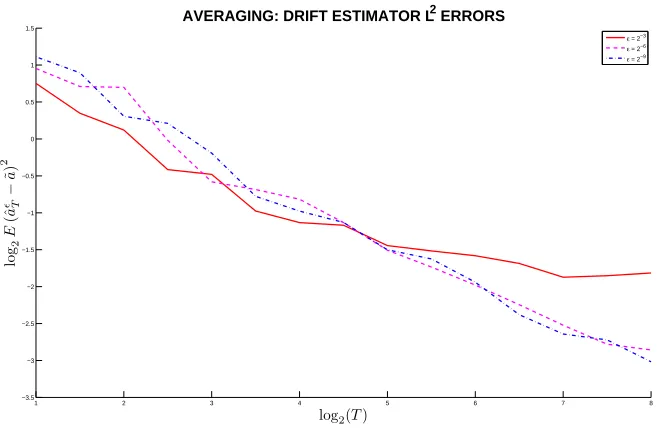
1 2 3 4 5 6 7 8 −3.5

−3 −2.5 −2 −1.5 −1 −0.5 0 0.5 1 1.5

log2(T)

log

2

E

(ˆ

a

ǫ−T

˜

a

)

2

AVERAGING: DRIFT ESTIMATOR L2 ERRORS

[image:38.595.156.486.112.329.2]

ε = 2−3 ε = 2−6 ε = 2−9

Figure 3.1: Averaging: Consistency of Estimatorˆaǫ_T

(ˆaǫ_T ₋˜a), in Figure 3.1. We see that when T = N δ is short, the estimation error from observations of different scale parameterǫ’s are similar. When time is large, the error with small scale parameterǫcontinues to decrease at a constant rate.

We then show the asymptotic variance of the estimator by plotting the distribution of the time adjusted errors√T(ˆaǫ_T −E_(ˆ_aǫ

T))withǫ= 2−9, in Figure 3.2. The asymptotic variance is computed using (3.13), which is 6 in our case. The red lines are the 2.5 and 97.5 quantiles of the adjusted errors, the blue lines are the expected confidence intervals of the adjusted errors. When observation timeT is large, the confidence intervals of the simulated errors are contained in the expected confidence intervals.

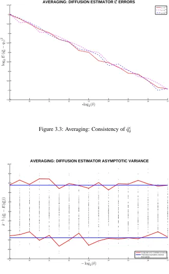
We then examine the convergence of the diffusion estimator in Theorem 3.9. We fix the total time horizonT =N δ= 1, and the scale parameterǫ= 2−9_,₂−6_and₂−3_{. We}

decrease the observation time incrementδ from2−9 to2−17. For each set of parameters, we sample 100 paths using the exact solution.

We first show the consistency of the estimator by plotting theL2_{norm of the errors}

(ˆq_δǫ₋q1), in Figure 3.3. We see that asδgets small, the estimation error from observations

of different scale parameterǫs are similar. This shows that the error is irrelevant to what value the scale parameter takes, and are always converging to zero.

We then show the asymptotic variance of the estimator by plotting the distribution of the δ adjusted errors δ−12(ˆqǫ

(39)

1 2 3 4 5 6 7 8 −10

−5 0 5

log2(T)

√

T

(ˆ

a

ǫ−T

E

(ˆ

a

ǫ))T

AVERAGING: DRIFT ESTIMATOR ASYMPTOTIC VARIANCE

[image:39.595.161.485.113.326.2]

Time adjusted error Confidence Interval Theoretical asymptotic variance Error points

Figure 3.2: Averaging: Asymptotic Normality ofˆaǫ_T

quantiles of the adjusted errors, the blue lines are the expected confidence intervals of the adjusted errors. We see that the confidence intervals of the simulated errors and and the expected confidence intervals agree.

3.8 Conclusion

In this chapter, we have verified asymptotic properties of the maximum likelihood estima-tors for the drift (2.5) and diffusion (2.6) parameters of an OU process, while observing data from the slow part of a multiscale system (3.1). We have verified that the discrepancy between the solution of the averaged equation (3.2) and the slow part of the system (3.1a), in theL2sense, is small whenǫis small. In summary,

• we take continuous observations from the multiscale system (3.1a)x;

• we have shown that the mismatch between trajectories ofxandXis asymptotically small ifǫis small;

• we have shown that the maximum likelihood estimatorˆaǫ_T converges to˜aasT → ∞

andǫ_→0, and the asymptotic distribution of the estimator;

• we have shown that the maximum likelihood estimatorqˆǫ

(40)

9 10 11 12 13 14 15 16 17 −7.5

−7 −6.5 −6 −5.5 −5 −4.5 −4 −3.5 −3 −2.5

-log2(δ)

log

2

E

(ˆ

q

ǫ−δ

q1

)

2

AVERAGING: DIFFUSION ESTIMATOR L2 ERRORS

[image:40.595.155.484.134.668.2]

ε = 2−3 ε = 2−6 ε = 2−9

Figure 3.3: Averaging: Consistency ofqˆǫ δ

9 10 11 12 13 14 15 16 17

−10 −8 −6 −4 −2 0 2 4 6 8 10

−log2(δ)

δ

−

1 2

(ˆ

q

ǫ−δ

E

(ˆ

q

ǫ))δ

AVERAGING: DIFFUSION ESTIMATOR ASYMPTOTIC VARIANCE

δ adjusted error Confidence Interval Theoretical asymptotic variance Error points

[image:40.595.158.489.134.347.2]

(41)

related toǫ;

(42)

Chapter 4

Parameter Estimation for the

Homogenized Equation of a

Multiscale OU Process

4.1 Introduction

In this chapter we consider the following fast/slow system of stochastic differential equa-tions

dx dt =

1

ǫ(a11x+a12y) + (a13x+a14y) +

√

q1

dU

dt (4.1a)

dy dt =

1

ǫ2 (a21x+a22y) +

r q2

ǫ2

dV

dt (4.1b)

for whichx_{∈ X} y _{∈ Y}. We may take_X asRd1 _and_Y _asRd2_{. The case where}_X _isTd1_, and_YisTd2 _{is discussed in [78]. We assume we observe data generated by the projection} onto thexcoordinate of the system. We also make the following assumptions.

Assumptions 4.1.

We assume that

(i) U, V are independent Brownian motions;

(ii) q1, q2 are positive definite diagonal matrices;

(43)

(iv) the system’s drift matrix

1

ǫa11+a13 1ǫa12+a14

1

ǫ2a21 _ǫ12a22

!

only have negative real eigenvalues whenǫis sufficiently small;

(v) a21invertible;

(vi) x(0)andy(0)are independent ofU andV,(x(0), y(0))is under the invariant mea-sure of system (3.1), andE _k_x₍₀₎_k2₊_k_y₍₀₎_k2_<_∞_.

Remark 4.2. In assumption 4.1(iv), we have assumed the whole system (4.1) to be ergodic

whenǫis sufficiently small. This condition can be decomposed toa22anda13−a14a−221a21

only have negative real eigenvalues; anda11−a12a−221a21= 0, which ensures the fast scale

term in (4.1a) vanishes.

Remark 4.3. Assumption 4.1(v) is necessary in our setup, however, the result could still

hold whena21has determinant zero, a scalar example is discussed by Papavasiliou in [20]

for diffusion estimates.

Remark 4.4. As in Remark 3.4 for the case of averaging,q1and q2 in Assumption 4.1(ii)

can also be relaxed to positive definite matrices to guarantee same result.

In what follows, we will refer to the following equation as the homogenized

equa-tion for system (4.1),

dX

dt = ˜aX+ p

˜

qdW

dt , (4.2)

where

˜

a=a13−a14a−221a21, (4.3)

and

˜

q=q1+a12a22−1q2a−221

∗

a∗₁₂. (4.4)

In the rest of this chapter,

• we take observations from the multiscale system (4.1a);

• we first show that the discrepancy between the trajectories from the slow partxof the multiscale system (4.1a) and the homogenized equation (4.2) is of orderO(ǫplog(ǫ))

in theL2_{sense, in Section 4.2;}

(44)

of the homogenized equation (4.2) in Section 4.3 by subsampling the observations at proper rates;

• we also show that using observations from the multiscale system (4.1a) and applying them to the diffusion estimatorˆσδ, defined in (2.6), we can correctly estimate the dif-fusion parameterq˜of the homogenized equation (4.2) in Section 4.4 by subsampling the observations at proper rates;

• finally a numerical example is studied to illustrate our findings in Section 4.5. The convergence of the homogenized system is different from that of the averaging systems. For each given time series of observations, the paths of the slow process converge to the paths of the corresponding homogenized equation. However, we will see that in the limitǫ _→ 0, the likelihood of the drift or diffusion parameter is different depending on whether we observe a path of the slow process generated by (4.1a) or the homogenized process (4.2) (see also [73, 78, 79]).

4.2 The Paths

The following theorem extends Theorem 18.1 in [78], which gives weak convergence of paths on Td_{. By limiting ourselves to the OU process, we extend the domain to}Rd _and

prove a stronger mode of convergence. We prove the following lemma first.

Lemma 4.5. Suppose that(x, y)solves (4.1a) and Assumptions 4.1 are satisfied. Then, for

fixed finiteT >0and smallǫ,

E _sup

0≤t≤T k

x(t)_k2+_ky(t)_k2=_O

log(1 + T

ǫ2)

(4.5)

where_k·kis the vector norm, and the order is in terms ofǫ. Proof. We look at the system of SDEs as,

dxt=axtdt+√qdWt (4.6) where,

x= x y

! ,a=

1

ǫa11+a13 1ǫa12+a14

1

ǫ2a21 _ǫ12a22 !

andq= q1 0

0 _ǫ12q2 !

.

We try to characterize the magnitude of the eigenvalues ofa. To find the eigenval-ues, we require

(45)

We either have the characteristic polynomial

det

1

ǫ2a22−λI

= 0,

or

det

(1

ǫa11+a13−λI)−(

1

ǫa12+a14)(

1

ǫ2a22−λI)−

1 1

ǫ2a21

= 0. First, we set the first determinant equal to zero:

det

1

ǫ2a22−λI

= 1

ǫ2d2 det a22−ǫ

2_λI_{= 0}_.

By definition, ǫ2λare the eigenvalues ofa22, thus they are of orderǫ2λ= O(1).

Conse-quently, we haved2(not necessarily distinct) real eigenvalues of orderO(_ǫ12). If the determinant of the second matrix is zero, we have

det

(1

ǫa11+a13−λI)−(

1

ǫa12+a14)(

1

ǫ2a22−λI)−

1 1

ǫ2a21

= 0. (4.7)

Rearranging the matrix we have,

det

(1

ǫa11+a13−λI)−(

1

ǫa12+a14)(a22−ǫ

2_λI₎−1_a

21

= 0.

We apply Taylor expansion onf(ǫ2) = (a22−ǫ2λI)−1atǫ= 0. We have,

f(ǫ2) =a−₂₂1+ǫ2λa−₂₂2+ǫ4λ2a−₂₂3+_O(ǫ6) =a₂₂−1+_O(ǫ2). We substitute the Taylor expansion into the determinant,

det

(1

ǫa11+a13−λI)−(

1

ǫa12+a14)(a22−ǫ

2_λI₎−1_a

21

= det

(1

ǫa11+a13−λI)−(

1

ǫa12+a14)(a

−1

22 +O(ǫ2))a21

= det

1

ǫ(a11−a12a−

1

22a21) + (˜a−λI) +O(ǫ)

= det ((˜a₋λI) +_O(ǫ)) = 0

It is equivalent to finding the eigenvalues of a perturbed matrix ofa. By Theorem 2 on page˜

137 in [42], on the eigenvalues of a perturbed matrix, we have that the corresponding d1

(46)

as

a=P DP−1withD=

D1 0

0 _ǫ12D2

!

whereDis the diagonal matrix, for whichD1 ∈ Rd1×d1 andD2 ∈ Rd2×d2 are diagonal

blocks of eigenvalues of orderO(1). We also define Σ = P−1q(P−1)∗. Using Lemma 9.14 in Appendix 9.11, we have the ratio between diagonal elements ofDandΣis always

Dii/Σii=O(1).

We apply Theorem 2.3 to the system of equations (4.6). We have

E _sup

0≤t≤Tk

x(t)k2 !

mini(|Dii/Σii|) .

SinceDii/Σii=O(1),maxi|Dii|=O(_ǫ12), we have

E _sup

0≤t≤Tk

x(t)k2 !

=_O

log(1 + T

ǫ2)

.

Sincex= x y

!

, we get

E _sup

0≤t≤T

(kx(t)k2+ky(t)k2)

!

=O

log

1 + T

ǫ2

.

Theorem 4.6. Let Assumptions 4.1 hold for system (4.1). Suppose thatxand X are

so-lutions of (4.1a) and (4.2) respectively. (x, y) corresponds to the realization (U, V) of Brownian motion, whileXcorresponds to the realization

W.= ˜q−12 √q₁U.−a₁₂a−1

22

√

q2V. (4.8)

andx(0) =X(0). Thenxconverges toXinL2_{. More specifically,}

E _sup

0≤t≤Tk

x(t)₋X(t)_k2_≤c

ǫ2log(T

ǫ) +ǫ

2_T

(47)

whenT is fixed finite, the above bound can be simplified to

E _sup

0≤t≤Tk

x(t)−X(t)k2 ₌_O₍_ǫ2_log(_ǫ₎₎_.

Proof. We rewrite (4.1b) as

(a−₂₂1a21x(t) +y(t))dt =ǫ2a−221dy(t)−ǫa22−1√q2dVt. (4.9) We also rewrite (4.1a) as

dx(t) = 1

ǫa12(a−

1

22a21x(t) +y(t))dt+a14(a−221a21x(t) +y(t))dt

+(a13−a14a−221a21)x(t)dt+√q1dUt

=

1

ǫa12+a14

(a−₂₂1a21x(t) +y(t))dt (4.10)

+˜ax(t)dt+√q1dUt.

Replacing(a−₂₂1a21x(t) +y(t))dtin (4.10) by the right-hand-side of (4.9), we get

dx(t) = ǫ(a12+ǫa14)a−221dy(t)−a12a−221√q2dVt−ǫa14a−221√q2dVt

+˜ax(t)dt+√q1dUt

= ˜ax(t)dt+ǫ(a12+ǫa14)a−₂₂1dy(t) (4.11)

+pqdW˜ t−ǫa14a−221

√

q2dVt. Thus

x(t) = x(0) +

Z t

0

˜

ax(s)ds+pqW˜ t (4.12)

+ǫ(a12+ǫa14)a−221(y(t)−y(0))−ǫa14a−221√q2Vt. Recall that the homogenized equation (4.2) is

X(t) =X(0) +

Z t

0

˜

aX(s)ds+pqW˜ t. (4.13)

Let e(t) = x(t)₋X(t). Subtracting the previous equation from (4.12) and using the assumptionX(0) =x(0), we find that

e(t) = ˜a Z t

0

e(s)ds (4.14)

+ǫ (a12+ǫa14)a−221(y(t)−y(0))−a14a−221

√

q2Vt

Parameter estimation and model fitting of stochastic processes

University of Warwick institutional repository: http://go.warwick.ac.uk/wrap

A Thesis Submitted for the Degree of PhD at the University of Warwick

http://go.warwick.ac.uk/wrap/51576

This thesis is made available online and is protected by original copyright.

Please scroll down to view the document itself.

Parameter Estimation and Model Fitting

of

Stochastic Processes

Fan Zhang

Contents

Acknowledgments

Declarations

Abstract

List of Figures

Chapter 1

Introduction

Part I

PARAMETER ESTIMATION FOR

MULTISCALE

ORNSTEIN-UHLENBECK

Chapter 2

The Ornstein-Uhlenbeck (OU)

Process

Chapter 3

Parameter Estimation for the

Averaged Equation of a Multiscale

OU Process

3.1

Introduction

3.2

The Paths

3.3

The Drift Estimator

3.4

Asymptotic Normality for the Drift Estimator

3.5

The Diffusion Estimator

3.6

Asymptotic Normality for the Diffusion Estimator

3.7

Numerical Example

3.8

Conclusion

Chapter 4

Parameter Estimation for the

Homogenized Equation of a

Multiscale OU Process

4.1

Introduction

4.2

The Paths