Perturbation resilience for the facility location problem

(1)

Discrete Mathematics and Mathematical Programming

MASTER’S THESIS

Perturbation resilience for

the facility location problem

M.B. Tijink

Supervisor:

Dr. B. Manthey (University of Twente, DMMP)

Graduation committee:

(2)

(3)

Abstract

Several NP-hard problems, e.g.𝑘-means clustering, are solved very quickly and near optimality

for practical instances, even though there are known worst-cases from a theoretical perspective. These worst-cases do not seem to appear in practice. There even is a saying; “Clustering is either easy or pointless”, indicating that the difficulty of these problems is only a theoretical concern. Several approaches to formalize this saying, by assuming that instances have a natural stability property in practice, recently proved to be successful in closing the gap between theory and practice.

In this thesis we look at the facility location problem, which is NP-hard. We add the𝛾-perturbation

resilience assumption, which requires that the instance must allow small perturbations of all costs in the instance without changing its optimal solution. Many instances in practice likely already satisfy this assumption, so we focus on the theoretical impact of this assumption. We found several consequences this assumption; local search algorithms will always result in the optimal solution, for𝛾 ≥ 3, and may not give the optimal solution for all𝛾 < 3. We also show

that several greedy algorithms do not work either to solve the facility location problem with the

𝛾-perturbation resilience assumption, even for high𝛾. A relation between this assumption and

approximation algorithms seems obvious, but we prove that this relation is false. Finally, we show that, for small𝛾, the existence of an efficient algorithm to solve the facility location problem with

(4)

(5)

1 Introduction

In this thesis we look at the facility location problem. This is a hard problem, as further explained in subsection 1.1, but the theoretical results for this problem show it to be more difficult than is observed in practice [17]. To solve this contrast between the theoretical and practical difficulty, we introduce the 𝛾-perturbation resilience assumption for the facility location problem (see

subsection 1.2): 𝛾-perturbation resilient instances of the facility location problem do not have

different optimal solutions when perturbed with small amounts. This assumption is somewhat natural: we think that many instances already have this property in practice, yet it makes the problem easier from the theoretical perspective. We will look into the consequences of making this assumption. In the following two subsections we will go into more detail about the facility location problem and the difference between NP-hardness in theory and practice, and we will detail the contributions made in this thesis in the final subsection.

1.1 The facility location problem

In the facility location problem we have a finite set of customers and a finite set of locations where we can open a facility. The goal of the facility location problem is to serve all customers while minimizing the total cost. This requires that each customer is connected to exactly one facility, which must be open. Thus, the key choice is which facilities to open and the secondary choice is which customer connects to which open facility. For every customer-location pair we have an associated cost, which we must pay if we we open a facility on that location and let the facility serve that customer. We also have associated costs for every location, which we must pay if we open a facility at that location. Thus, there is a tradeoff between opening many facilities such that the customer-location costs stay low and opening few facilities such that the facility costs are low. A common application of the facility location problem is determining where to build e.g. warehouses or hospitals. For more details on the facility location problem, see Krarup and Pruzan [20] or Melo et al. [25].

A lot of variants of this simple problem exist. For example, the uncapacitated facility location problem, as described above, allows an arbitrary number of customers to connect to an open facility. Thus, facilities must be very flexible, but this is not realistic for all application. The capacitated facility location problem limits the number of customers to connect to an open facility. This way you could, for example, limit a warehouse capacity to five customers. If the capacity is reached, another facility needs to be opened to serve the remaining customers, either at the same location or at another location. The metric facility location problem requires the customer-location costs to be metric, making them behave like distances. This variant is suitable when the distance or time used in a road network is important. The non-metric facility problem does not restrict the customer-location costs, making it more suited for optimizing other types of resources. Some facility location problem variants have per-customers demands and per-unit customer-location prices, instead of just a single customer-location cost. This may not seem useful on its own, but is useful when combined with e.g. the metric facility location problem, as the demand and unit price formulation of the facility location problem allows more instances when these prices must be metric. And, of course, these variants can usually be combined for even more variants of the facility location problem [25, 32].

The facility location problem can also be seen as a variant of the𝑘-means problem, but with

variable amount of cluster centers to open and costs depending on which cluster center you open [11, 12, 24].

(8)

The uncapacitated non-metric facility location problem is even NP-hard to approximate within a factor𝑂(log |𝐷|), where|𝐷|is the number of customers [28, 32], so even guaranteeing a good

solution is a hard problem.

The uncapacitated metric facility location problem, which we use in this thesis, is NP-hard to approximate within a factor 1.463 [16]. On the other hand, there are approximation algorithms that guarantee a solution within a factor 1.5 of the optimal solution [10].

1.2 NP-hardness in practice

Problems in computer science, e.g. the shortest path problem or the traveling salesman problem, can be classified depending on how fast they can be solved, for the fastest algorithm which solves them. So even if a problemAhas a very slow algorithm, there could also be faster algorithms, so

Adoes not need to be classified corresponding with the slow algorithm. The most well known complexity classes are P, meaning Polynomial, and NP, meaning Nondeterministic Polynomial. If a problemAis in P, there is an algorithm that solvesAin polynomial time, for any possible instance ofA. Problems in NP can be solved in non-deterministic polynomial time or, equivalently, solutions to problems in NP can be verified in polynomial time given a proof of the solution [15, 27]. We often say a problemAin P is easy or that it has an efficient algorithm. On the other hand, we call call a problemAhard or say that it has only inefficient known algorithms if Ais in NP. Other complexity classes also exist, for example we use complexity class RP, meaning Randomized Polynomial, in this thesis. Algorithms for problems in RP can use random numbers, so their output is not necessarily deterministic. An algorithm for some problemAin RP must always answer no if the given instance ofAhas no as answer, and the algorithm must answer yes with probability at least 1

2 if the answer is yes. [27].

Proving that a problem is at least as hard as other problems is usually done with reductions. A reduction transforms instances of some problemBto an instance of some problemAsuch that the answer to the instance of problemBis identical to the answer of transformed instance. This way, if you have algorithm which can solveA, you can solveBby first running the transformation and then solving the resulting instance of problemA. Thus, a reduction proves that problemBis at least as hard as problemA[15, 27].

Cook showed that every problem in NP can be reduced to the boolean satisfiability problem [13], making it the first so-called NP-complete problem. If you prove that an NP-complete problem is in P, you have proved that P=NP. Likewise if you prove that an NP-complete problem is not in

P, you have proved that P≠NP. Thus, NP-complete problems can be seen as a characterization

of NP. Using a reduction from an NP-complete problemBto some other problemAin NP proves thatAalso is NP-complete. Examples of NP-complete problems are the SAT, clique, traveling salesman and knapsack problems [19]. The facility location problem is also NP-complete [20]. Despite all the research being done on those problems, to date no algorithms have been found to solve these problems in deterministic polynomial time; the question “P=NP or P≠NP?” is

still open. For optimization problems, where the goal is to find the optimal solution, this is even worse: some problems of approximation, where the goal is to find a solution with value within a certain factor of the optimal solution, are still NP-hard, e.g. for the facility location problem and traveling salesman problem [14, 16].

(9)

1. Introduction

inherent properties making them easier. The first of those reasons gave rise to smoothed analysis, in which small random perturbations are applied to instances. The idea in smoothed analysis is that the difficult instances are so specific that nearly all similar instances are not very difficult. This has been successfully applied to e.g. the simplex algorithm [30] and the 2-OPT heuristic for the traveling salesman problem [22].

Another approach to better understand and analyze NP-hard problems is to constrain which instances are allowed. Examples of this approach are looking only at planar graphs instead of all graphs, or looking at the traveling salesman problem with metric distances. This yields useful results, but is generally not applicable in practice since real-world instances do not have those properties. A more recent approach is to choose a assumption on the allowed instances which is true, close to true or often true in practice [9]. An example where this approach was used is for MAX-CUT, where instances which are stable under perturbation can be solved efficiently [8]. Graph coloring is efficiently solvable if you assume that adding a couple of edges at arbitrary places in the graph does not increase its chromatic number [21]. The traveling salesman problem becomes easier if its optimal solution is some factor better than non-optimal solutions [26]. The most research with these kinds of assumptions has been done on the (𝑘-means) clustering problem,

with several approaches [1, 4, 5, 6, 7, 29].

In the 𝑘-means clustering problem you have a set of points which you have to divide into 𝑘

clusters. Equivalently, you can choose𝑘cluster centers, as these directly correspond to clusters,

and vice versa. The goal is to find clusters that minimize the sum of distances from point to its assigned cluster center. Awasthi et al. looked at𝛾-perturbation stability for clustering: if you

assume that the𝑘-means instance has the same optimal solution after arbitrary perturbations of

at most a factor𝛾, then finding this solution is relatively easy [4].

As the facility location problem can be seen as a variant of the𝑘-means clustering problem, we

will use a𝛾-perturbation resilience assumption similar to Awasthi et al. in this thesis. It seems

likely that many real-world instances already satisfy this𝛾-perturbation resilience, for small𝛾. In

this thesis we will see how the𝛾-perturbation resilience assumption makes the facility location

problem easier.

1.3 Contributions made in this thesis

In this thesis we first look at the facility location problem in general, before adding the

𝛾-perturbation resilience assumption and seeing what basic consequences this has (Section 2).

Then we look at several reasons why the facility location problem becomes somewhat easier with

𝛾-perturbation resilience. The first such reason is that local search algorithms will always find the

optimal solution for𝛾-perturbation resilient instances with𝛾 ≥ 3. On the flip side, there exist (3 − 𝜀)-perturbation resilient instances that have local minima not equal to the optimal solution

(Section 3). Several greedy algorithms have similar problems for small 𝛾, as we will show: these

greedy algorithms make mistakes while determining the solution, even for𝛾-perturbation resilient

instances with relatively high𝛾(Section 4). This turns out to happen even for one of the currently

best performing approximation algorithms, the Jain-Mahdian-Saberi algorithm [17]. This is a surprise, since a connection between 𝛾-perturbation resilience and approximation algorithms

seems obvious. We prove that this connection is unfounded with a counterexample (Section 5). We also look at how hard the facility location problem is with 𝛾-perturbation resilience, and

found that if the ability to solve the perturbation resilient facility location problem for small𝛾

(10)

(11)

2. The facility location problem

2 The facility location problem

The facility location problem has several variants. The variant we use in this thesis is usually called the uncapacitated metric facility location problem:

Definition. Theuncapacitated metric facility location problem(referred to as thefacility location problem or theFLP in this thesis) is the following optimization problem.

Instance: an instance(𝐹 , 𝐷, 𝑓, 𝑐) of the FLP consists of a finite set of locations𝐹, a finite set

of customers 𝐷, facility costs 𝑓𝑖≥ 0 for all𝑖 ∈ 𝐹 and service costs 𝑐𝑖𝑗≥ 0 for all𝑖 ∈ 𝐹 , 𝑗 ∈ 𝐷.

The service costs are metric, i.e.𝑐𝑖𝑗≤ 𝑐𝑖′_𝑗+ 𝑐_𝑖′_𝑗′+ 𝑐_𝑖𝑗′ for all 𝑖, 𝑖′∈ 𝐹 , 𝑗, 𝑗′∈ 𝐷.

Solutions: a solution (𝑋, 𝜎)for an instance (𝐹 , 𝐷, 𝑓, 𝑐)of the FLP consists of a nonempty set

of open facilities 𝑋 ⊆ 𝐹and a customer assignment𝜎 ∶ 𝐷 → 𝑋to open facilities.

Objective: The cost of a solution is𝑐(𝑋, 𝜎) = ∑_𝑖∈𝑋𝑓𝑖+∑𝑗∈𝐷𝑐𝜎(𝑗)𝑗. The objective is to minimize

𝑐(𝑋, 𝜎).

This variant is called uncapacitated since all facilities can handle an arbitrary number of customers and it is called metric because the service costs satisfy an extension of the triangle inequality. The optimal solution to an FLP instance is usually denoted as(𝑋∗_{, 𝜎}∗₎_{. The solution costs of the} FLP,𝑐(𝑋, 𝜎), can be split into two parts: the facility costs 𝑐𝐹(𝑋) = ∑𝑖∈𝑋𝑓𝑖and service costs

𝑐𝑆(𝑋, 𝜎) = ∑𝑗∈𝐷𝑐𝜎(𝑗)𝑗. Additionally, given an instance of the FLP and a set of open facilities 𝑋, it is easy to compute an optimal corresponding customer assignment𝜎: 𝜎(𝑗) = arg min_𝑖∈𝑋𝑐𝑖𝑗,

breaking ties arbitrarily. Thus, the customer assignment is often dropped in the cost notations, which implies that an optimal assignment is used.

Besides the metric FLP, as defined above, we sometimes use the non-metric version of the FLP in this thesis:

Definition. The uncapacitated facility location problem(referred to as the non-metric FLPin this thesis) is identical to the FLP except for one detail: an instance(𝐹 , 𝐷, 𝑓, 𝑐)of the non-metric

FLP has service costs which need not be metric, i.e. 𝑐𝑖𝑗≰ 𝑐𝑖′_𝑗+ 𝑐_𝑖′_𝑗′+ 𝑐_𝑖𝑗′ is allowed. Thus, an instance of the FLP is also an instance of the non-metric FLP.

2.1 Results on the facility location problem

There is a decision variant of the FLP, where for a given instance(𝐹 , 𝐷, 𝑓, 𝑐)and bound𝐿the

question is whether the optimal solution𝑋∗ _{has cost}_𝑐(𝑋∗_{) ≤ 𝐿}_{. This decision variant of the} FLP is NP-complete, as we will show in the following theorem and proof (for more information, see Krarup et al. [20]).

Theorem 1. The decision variant of the FLP is NP-complete.

Proof. First, we show that the decision variant of the FLP is in NP. For an arbitrary given instance(𝐹 , 𝐷, 𝑓, 𝑐)and bound𝐿, choose an arbitrary nonempty set𝑋 ⊆ 𝐹nondeterministically.

Now check if the cost𝑐(𝑋) ≤ 𝐿. If so, output “yes”, otherwise, output “no”.

If the instance has 𝑐(𝑋∗_{) ≤ 𝐿}, this will output “yes”, since _𝑋∗ _{⊆ 𝐹} and_𝑋∗ is nonempty, so it will be one of the nondeterministic choices. If the instance has 𝑐(𝑋∗_{) > 𝐿}_{, then because}

(12)

Now, to show that the decision variant of the FLP is NP-hard, we reduce the set-covering problem to the FLP. Because the decision variant of the set-covering problem is NP-complete [19], this will prove that the decision variant of the FLP is NP-hard.

The instances (𝑈 , 𝑆)of the set-covering problem consist of the universe𝑈 and a collection of

subsets𝑆 = ⋃ 𝑆𝑖, where each𝑆𝑖 is a subset of𝑈. The goal of the set-covering problem is to find the minimum cardinality set𝐶 ⊆ 𝑆that covers𝑈, i.e. {𝑥 ∣ 𝑥 ∈ 𝑆𝑖, 𝑆𝑖∈ 𝐶for some 𝑖} = 𝑈. Given an instance(𝑈 , 𝑆)and bound𝑘, construct the following FLP instance and bound:

𝐹 = 𝑆, 𝐷 = 𝑈 , 𝑓𝑖= 1,

𝑐𝑖𝑗= {

𝑘 if𝑗 ∈ 𝑖, and 3𝑘 otherwise, 𝐿 = 𝑘 + 𝑘|𝐷|.

Clearly, if (𝑈 , 𝑆) is a yes-instance, so is (𝐹 , 𝐷, 𝑓, 𝑐), by opening facilities 𝑋 = 𝐶, yielding 𝑐(𝑋) = |𝐶|+𝑘|𝐷| ≤ 𝑘+𝑘|𝐷| = 𝐿. If(𝐹 , 𝐷, 𝑓, 𝑐)is a yes-instance, some𝑋has𝑐(𝑋) ≤ 𝐿 = 𝑘+𝑘|𝐷|,

so𝑐𝜎(𝑗)𝑗= 𝑘for every𝑗 ∈ 𝐷. Thus,𝐶 = 𝑋is a set cover with|𝐶| = 𝑐(𝑋) − 𝑘|𝐷| ≤ 𝑘and(𝑈 , 𝑆) is a yes-instance. As a result, this is a valid reduction, proving that the decision variant of the FLP is NP-hard.

As a consequence of this theorem, the (search variant of the) FLP is NP-hard.

NP-hard optimization problems often still have approximation algorithms which run in determin-istic polynomial time, which give a solution with cost at most a factor𝛼 > 1times the optimal

cost. Depending on the problem, there may be a lower bound for𝛼, below which the problem

is still NP-hard. The following three theorems show the current best approximation hardness results for the FLP.

Theorem 2 (Guha and Kuller 1999 [16]).Approximating the FLP within a factor𝛼 = 1.463

is NP-hard.

Theorem 3 (Byrka and Aardal 2010 [10]). The FLP can be approximated within a factor

𝛼 = 1.5by a deterministic polynomial time algorithm.

Theorem 4 (Li 2013 [23]).The FLP can be approximated with a expected factor 𝛼 = 1.488by

a randomized polynomial time algorithm, i.e. for any possible instance, the algorithm computes solutions 𝑋such that 𝔼[𝑐(𝑋)] ≤ 1.488𝑐(𝑋∗₎_.

These results are not particularly promising if you want to find a good solution to your FLP instance, since solutions 50% more expensive than the optimal solution does not seem very attractive. However, in practice several of the best approximation algorithms do a lot better. For example, the Jain-Mahdian-Saberi algorithm, with an approximation ratio𝛼 = 1.61, achieves

a ratio of 1.03 on average on real-world instances [17]. This difference between the observed performance and guaranteed performance leads us to making an assumption about real-world instances, as we show in the next subsection.

2.2 Perturbation resilience

(13)

perturbation resilience assumption for clustering problems by Awasthi et al. [4], adapted to the FLP, looks like a good choice. First, we need to define what it means to perturb an FLP instance. Definition. An instance (𝐹 , 𝐷, 𝑓′_{, 𝑐}′₎ of the non-metric FLP is a _γ-perturbation of instance

(𝐹 , 𝐷, 𝑓, 𝑐) of the FLP, with 𝛾 ≥ 1, iff 𝑓𝑖 ≤ 𝑓𝑖′ ≤ 𝛾𝑓𝑖 for all𝑖 ∈ 𝐹 and 𝑐𝑖𝑗 ≤ 𝑐′𝑖𝑗 ≤ 𝛾𝑐𝑖𝑗 for all

𝑖 ∈ 𝐹 , 𝑗 ∈ 𝐷. If it is clear from the context which𝐹and𝐷 are used, a𝛾-perturbed instance can

also be denoted as (𝑓′_{, 𝑐}′₎_.

A𝛾-perturbed instance is any instance that is a𝛾-perturbation of some FLP instance.

Note that a 𝛾-perturbed instance might or might not be metric. This definition only allows

greater costs than the original instance, which might seem weird for a perturbation, but this is simply a matter of scaling. An FLP instance remains equivalent under scaling all costs with the same value, so an equivalent definition of 𝛾-perturbation also allowing lower costs would, for

instance, be: 𝑓𝑖≤

√ 𝛾𝑓′

𝑖 ≤ 𝛾𝑓𝑖 and similar for the service costs.

Using this definition, we can define𝛾-perturbation resilience for the FLP.

Definition. An instance (𝐹 , 𝐷, 𝑓, 𝑐) of the FLP is γ-perturbation resilient with 𝛾 ≥ 1 iff all 𝛾-perturbations(𝑓′_{, 𝑐}′₎_of _{(𝐹 , 𝐷, 𝑓, 𝑐)}_{have the same unique optimal solution}_(𝑋∗_{, 𝜎}∗₎_.

For small 𝛾(i.e.𝛾 < 1.05or similar), it seems likely that many real-world instances satisfy this

assumption, since stability of solutions makes a lot of sense: if an instance is very sensitive to perturbations, then it means that the exact solution probably does not matter much. For small𝛾,

it also implies that the instance is resilient in the face of small changes to the costs. In practice, this often happens too: you are not going to change the location of your warehouse if it is 3% farther away than previously estimated. Nevertheless, we will consider all values𝛾in this thesis.

In the conclusion (section 7) we will come back to the results and see if they are applicable in practice.

If costs of𝛾-perturbed instances are compared, the notation of the perturbed costs follow from

the names given to the perturbed instances. So, for example, if(𝑓′_{, 𝑐}′₎is a_𝛾-perturbed instance, then𝑐′_(𝑋)_{denotes the cost of solution}_𝑋_{in the perturbed instance.}

Any𝛾-perturbation resilient instance of the FLP is a valid𝛾-perturbation of itself, so𝛾-perturbation

resilience implies that the original instance has the same optimal solution as any of its perturbations. Note that, since𝛾-perturbation resilience requires an unique solution, there are instances of the

FLP which are not𝛾-perturbation resilient for any𝛾, namely exactly those instances with multiple

optimal solutions.

The definition of𝛾-perturbation resilience, although intuitive, is somewhat hard to work with

since it requires checking the optimal solution for all 𝛾-perturbations of an FLP instance. The

following theorem introduces an equivalent but easier to check definition.

Theorem 5. Consider, for some instance (𝐹 , 𝐷, 𝑓, 𝑐) of the FLP with optimal solution 𝑋∗_,

customer assignment𝜎∗ _{and nonzero optimal cost}_𝑐(𝑋∗₎_{, the following} _𝛾_{-perturbation:}

𝑓′ 𝑖 = {

𝛾𝑓𝑖 if𝑖 ∈ 𝑋∗, and

𝑓𝑖 otherwise,

𝑐′ 𝑖𝑗= {

𝛾𝑐𝑖𝑗 if𝜎∗(𝑗) = 𝑖, and

𝑐𝑖𝑗 otherwise.

This𝛾-perturbed instance(𝐹 , 𝐷, 𝑓′_{, 𝑐}′₎_{has the same optimal solution}_𝑋∗_{and customer assignment}

𝜎∗ _{iff the instance}_{(𝐹 , 𝐷, 𝑓, 𝑐)}_is _𝛾_{-perturbation resilient. If so, the solution} _(𝑋∗_{, 𝜎}∗₎_{is unique for}

(14)

Proof. If the instance is 𝛾-perturbation resilient, then the given 𝛾-perturbation has the same

unique optimal solution, by definition of𝛾-perturbation resilience.

Thus, assume that the solution (𝑋∗_{, 𝜎}∗₎_{is also the solution to the given}_{(𝐹 , 𝐷, 𝑓}′_{, 𝑐}′₎_instance. Consider all possible𝛾-perturbations( ̃𝑓, ̃𝑐)of the(𝐹 , 𝐷, 𝑓, 𝑐)instance and construct the following 𝛾-perturbation:

̃

𝑓′ 𝑖 = {

̃

𝑓𝑖 if𝑖 ∈ 𝑋∗, and

𝑓𝑖 otherwise,

̃

𝑐′ 𝑖𝑗= {

̃

𝑐𝑖𝑗 if𝜎∗(𝑗) = 𝑖, and

𝑐𝑖𝑗 otherwise.

By construction, it holds that𝑐(𝑋̃ ∗_{, 𝜎}∗_{) = ̃}_𝑐′_(𝑋∗_{, 𝜎}∗₎ and_𝑐′_̃_{(𝑋, 𝜎) ≤ ̃}_{𝑐(𝑋, 𝜎)} for all nonempty open facility sets𝑋 ⊆ 𝐹and customer assignments𝜎 ∶ 𝐷 → 𝑋. Now relate𝑐′_(𝑋∗_{, 𝜎}∗₎to_𝑐′_̃_(𝑋∗_{, 𝜎}∗₎ and𝑐′_{(𝑋, 𝜎)} _to_𝑐′_̃_{(𝑋, 𝜎)}_:

𝑐′_(𝑋∗_{, 𝜎}∗_{) = ̃}_𝑐′_(𝑋∗_{, 𝜎}∗_{) + ∑} 𝑖∈𝑋∗

𝛾𝑓𝑖− ̃𝑓𝑖+ ∑ 𝑗∈𝐷

𝛾𝑐𝜎∗_(𝑗)𝑗− ̃𝑐_𝜎∗_(𝑗)𝑗, (1)

𝑐′_{(𝑋, 𝜎) = ̃}_𝑐′_{(𝑋, 𝜎) + ∑} 𝑖∈𝑋∩𝑋∗

𝛾𝑓𝑖− ̃𝑓𝑖+ ∑ 𝑗∈𝐷 𝜎(𝑗)=𝜎∗_(𝑗)

𝛾𝑐𝜎∗_(𝑗)𝑗− ̃𝑐_𝜎∗_(𝑗)𝑗. (2)

By assumption 𝑐′_(𝑋∗_{, 𝜎}∗_{) < 𝑐}′_{(𝑋, 𝜎)}_{. So} _𝑐′_̃_(𝑋∗_{, 𝜎}∗_{) <} _𝑐′_̃_{(𝑋, 𝜎)}_{, because the sum terms in} equation (1) are at most the sum terms in equation (2). As noted above, by construction it follows that𝑐(𝑋̃ ∗_{) < ̃}_𝑐(𝑋)_.

This holds for all𝛾-perturbations( ̃𝑓, ̃𝑐)of(𝐹 , 𝐷, 𝑓, 𝑐)and all solutions(𝑋, 𝜎). Because𝑐(𝑋∗_{) ≠ 0} the solution is unique, proving that the instance(𝐹 , 𝐷, 𝑓, 𝑐)is𝛾-perturbation resilient.

We now have two equivalent definitions for𝛾-perturbation resilience, so it is useful to know for

which range of𝛾 𝛾-perturbation resilient instances exist. FLP instances need to be metric, so this

is not a trivial fact. The following two theorems establish that𝛾-perturbation resilient instances

exist for all𝛾 ≥ 1.

Theorem 6.If an FLP instance (𝐹 , 𝐷, 𝑓, 𝑐)is𝛾-perturbation resilient, it also is𝛾′_{-perturbation}

resilient for all 𝛾′_∈_ℝ _{which satisfy}_{1 ≤ 𝛾}′_{≤ 𝛾}_.

Proof. Let (𝐹 , 𝐷, 𝑓, 𝑐) be any possible 𝛾-perturbation resilient FLP instance, and 𝛾′ _∈ _ℝ _be an arbitrary number which satisfies 1 ≤ 𝛾′ _{≤ 𝛾}_{. Now consider all} _𝛾′ _{perturbations} _(𝑓′_{, 𝑐}′₎ of (𝐹 , 𝐷, 𝑓, 𝑐). Since 𝛾′ _{≤ 𝛾}_, _(𝑓′_{, 𝑐}′₎_{is a valid} _𝛾_{-perturbation of} _{(𝐹 , 𝐷, 𝑓, 𝑐)}_{. By definition of}

𝛾-perturbation resilience, this implies that the same solution is the unique optimal solution to

both(𝐹 , 𝐷, 𝑓, 𝑐)and(𝑓′_{, 𝑐}′₎_.

This satisfies the requirement for𝛾′_{-perturbation resilience, proving the theorem.}

Theorem 7.For all 𝑥 ∈ℝ, there exist𝛾-perturbation resilient instances of the FLP with𝛾 > 𝑥.

(15)

generality. Now consider the following instance (see Figure 1):

𝐹 = {1𝑓, 2𝑓},

𝐷 = {1𝑑, 2𝑑},

𝑓𝑖= 0,

𝑐𝑖𝑗= {

1 if𝑖 = 𝑘𝑓, 𝑗 = 𝑘𝑑 for some𝑘, and

2𝑥 otherwise.

1𝑓

2𝑓

1𝑑 2𝑑

𝑐1𝑓1𝑑

= 1 𝑐1_𝑓₂

𝑑 = 2𝑥

𝑐₂ 𝑓1_𝑑 _{= 2𝑥}

𝑐2𝑓2𝑑 = 1 𝑓1𝑓= 0

𝑓2𝑓= 0

Figure 1: Example of Theorem 7

This instance has three possible solutions, with the following costs:

𝑐({1𝑓}) = 2𝑥 + 1,

𝑐({2𝑓}) = 2𝑥 + 1,

𝑐({1𝑓, 2𝑓}) = 2.

Since all 𝛾-perturbations increase the cost of a solution 𝑋 at most by a factor 𝛾, a trivial

lower bound for the perturbation resilience 𝛾′ _{of this instance can be calculated as follows:}

𝛾′₌2𝑥+1 2 = 𝑥 +

1

2. This is a contradiction to the assumption that all instances of the FLP are

𝛾-perturbation resilient with𝛾 < 𝑥, since𝛾′_{> 𝑥}_.

For most NP-hard problems, it is trivial to find the optimal solution to an instance once you have an algorithm that solves the decision variant of the problem (i.e. “is the cost of the optimal solution below a given bound?”). The following theorem looks at the decision variant of the FLP for𝛾-perturbation resilient instances.

Theorem 8.Assume a deterministic algorithm A exists that decides 𝑔(|𝐹 |, |𝐷|)-perturbation

resilient FLP instances(𝐹 , 𝐷, 𝑓, 𝑐)in polynomial time, for some function𝑔. Then a deterministic

algorithm exists that finds the optimal solution𝑋∗ _for_𝛾′_{-perturbation resilience FLP instances}

(𝐹 , 𝐷, 𝑓, 𝑐)with𝛾′_{> 𝑔(|𝐹 |, |𝐷|)} _{in polynomial time.}

This theorem implies that, like for many other NP-hard problems, discovering the value of a 𝛾-perturbation resilient instance is not more difficult than finding the corresponding

solu-tion. The only exception, where this may or may not be true, is the border case of exactly

𝑔(|𝐹 |, |𝐷|)-perturbation resilient instances. Although a theorem like this for general FLP can

easily be proven using self-reducibility, this is not true here. Self-reducibility can destroy the

𝛾-perturbation resilience of an instance, and as result the assumed existing algorithm cannot be

applied to the resulting instances.

(16)

Because𝛾′_{> 𝑔(|𝐹 |, |𝐷|)}_{, it is possible to} 𝛾′

𝑔(|𝐹 |,|𝐷|)-perturb the instance(𝐹 , 𝐷, 𝑓, 𝑐)to some instance

(𝐹 , 𝐷, 𝑓′_{, 𝑐}′₎_{. Because this is a valid} _𝛾′_{-perturbation, both instances yield the same optimal} solution 𝑋∗ _{and customer assignment}_𝜎∗_{. Note that all} _{𝑔(|𝐹 |, |𝐷|)}_{-perturbations of instance}

(𝐹 , 𝐷, 𝑓′_{, 𝑐}′₎_{are valid}_𝛾′_{-perturbations of}_{(𝐹 , 𝐷, 𝑓, 𝑐)}_{. Thus, algorithm}_A_{can be used on all such} instances(𝐹 , 𝐷, 𝑓′_{, 𝑐}′₎_{, since they are}_{𝑔(|𝐹 |, |𝐷|)}_{-perturbation resilient, and use the same optimal} solution𝑋∗ _{to decide if it is a yes- or no-instance.}

So, consider the following 𝛾′

𝑔(|𝐹 |,|𝐷|)-perturbation, for some fixed facility 𝑖

′ _{∈ 𝐹}_{, which will be} chosen later:

𝑓′ 𝑖 = {

𝛾′

𝑔(|𝐹 |,|𝐷|)𝑓𝑖 if𝑖 = 𝑖 ′_{, and}

𝑓𝑖 otherwise.

This perturbed instance(𝐹 , 𝐷, 𝑓′_{, 𝑐)}_{has cost}_𝑐′_(𝑋∗_{) = 𝑐(𝑋}∗₎_iff_𝑖′_{∉ 𝑋}∗_{. So by running algorithm}

Aon instance(𝐹 , 𝐷, 𝑓′_{, 𝑐)}_{with threshold}_𝑐(𝑋∗₎_{, a part of the optimal solution}_𝑋∗ _{is discovered,} if𝑓𝑖′= 0. If𝑓_𝑖′= 0, we know that including𝑖′ in𝑋∗ never results in a higher cost. Doing this for all facilities𝑖′_{∈ 𝐹}yields the optimal solution_𝑋∗.

(17)

3. Local search

3 Local search

Local search techniques are a common way to solve problems. In a local search algorithm, we always start from some initial solution, like a trivial solution (e.g. 𝑋 = 𝐹 for the FLP) or a

solution computed by a heuristic. From there, local search tries to improve its current solution. It does that by computing the neighbourhood of the current solution, a set of solutions which are similar to the current solution. What this neighbourhood is differs per problem and can be chosen by the creator of the local search algorithm. The local search algorithm now computes the cost of each solution in the neighbourhood. If at least one is better than the current solution, it updates its current solution to one of the better solutions. If none are, the local search algorithm terminates. All solutions which are at least as good as all their neighbouring solutions are called local minima.

Local search techniques are commonly used in practice, since they are easy to implement: they only require you to define a neighbourhood, which is quite simple. Additionally, real-world problems often have extra constraints on the solution, which do not correspond to the theoretical problems. An example for the FLP would be that there are a few facilities that, when open, must have exactly three assigned customers. These extra constraints are not difficult to add in a local search algorithm.

In this section we look at local minima and local search algorithms in general, and see how

𝛾-perturbation resilient instances impact them.

3.1 Existence of local minima

In this subsection we will show that 3-perturbation resilient instances do not have local minima except for the global minimum. We also show that there are(3−𝜀)-perturbation resilient instances

for which this is not true, i.e. that there are local minima unequal to the optimal solution. To do so, we first define what a local minimum is for the FLP.

Definition. A solution𝑋to an instance of the FLP is a local minimum iff

• 𝑐(𝑋⧵{𝑖}) ≥ 𝑐(𝑋) for all 𝑖 ∈ 𝑋with|𝑋| ≥ 2(dropping a facility), and

• 𝑐(𝑋 ∪ {𝑖}) ≥ 𝑐(𝑋)for all𝑖 ∈ 𝐹⧵𝑋 (adding a facility), and

• 𝑐(𝑋⧵{𝑖} ∪ {𝑗}) ≥ 𝑐(𝑋) for all𝑖 ∈ 𝑋, 𝑗 ∈ 𝐹⧵𝑋 (swapping a facility).

This definition means that the local minimum𝑋cannot be improved by opening a new facility,

closing an open facility or switching between an open and closed facility.

The following theorem is a result for local search algorithms on any FLP instance.

Theorem 9 (Arya et al. 2004 [3]). All local minima 𝑋 for an instance of the FLP satisfy 𝑐𝐹(𝑋) ≤ 𝑐𝐹(𝑋∗) + 2𝑐𝑆(𝑋∗)and𝑐𝑆(𝑋) ≤ 𝑐𝐹(𝑋∗) + 𝑐𝑆(𝑋∗), where𝑋∗ is the optimal solution for

the instance. Combined, this yields𝑐(𝑋) ≤ 3𝑐(𝑋∗₎_.

This theorem will be used to show that there are no local minima except for the optimal solution for 3-perturbation resilient FLP instances (Theorem 11). To prove this, we first need an extra result from the following lemma. This lemma means that, if some𝛾-perturbation resilient instance

exists, then also such a𝛾-perturbation resilient instance with more restrictions exists: you can

see this as removing everything from an instance that is not needed to remain𝛾-perturbation

(18)

Lemma 10.Assume a𝛾-perturbation resilient instance(𝐹 , 𝐷, 𝑓, 𝑐)of the FLP exists with a local

minimum(𝑋, 𝜎) not equal to the optimal solution(𝑋∗_{, 𝜎}∗₎_.

Then an instance (𝐹′_{, 𝐷}′_{, 𝑓}′_{, 𝑐}′₎_{of the FLP exists with the following properties:}

• the instance(𝐹′_{, 𝐷}′_{, 𝑓}′_{, 𝑐}′₎_is_𝛾_{-perturbation resilient, and}

• the instance(𝐹′_{, 𝐷}′_{, 𝑓}′_{, 𝑐}′₎_{has a local minimum}_(𝑋′_{, 𝜎}′₎_{not equal to the optimal solution}

(𝑋′∗_{, 𝜎}′∗₎_{, and}

• 𝐹′_{= 𝑋}′_{∪ 𝑋}′∗, and

• 𝑓′

𝑖 = 0for all 𝑖 ∈ 𝑋′∩ 𝑋′∗, and

• for all 𝑗 ∈ 𝐷′_{, (}_𝜎′_{(𝑗) ∉ 𝑋}′_{∩ 𝑋}′∗ _or_𝜎′∗_{(𝑗) ∉ 𝑋}′_{∩ 𝑋}′∗_).

Note that the optimal solution (𝑋∗_{, 𝜎}∗₎_{to any instance is always a local minimum, so this is} explicitly excluded in the lemma.

Proof. Take any such instance(𝐹 , 𝐷, 𝑓, 𝑐). We transform the instance(𝐹′_{, 𝐷}′_{, 𝑓}′_{, 𝑐}′₎using the following steps. We apply each step until its conditions are satisfied for all local minima𝑋 ≠ 𝑋∗, possibly applying earlier steps again in the process if their conditions are not valid any more after applying a later step. Thus, at the beginning of every step, the conditions of all previous steps are satisfied.

Step 1. Condition to satisfy: 𝐹 = 𝑋 ∪ 𝑋∗_.

Drop all facilities not in𝑋or𝑋∗, i.e._𝐹′_{= 𝑋 ∪ 𝑋}∗. All customer assignments of_𝜎and_𝜎∗ remain valid and the costs 𝑐(𝑋)and 𝑐(𝑋∗₎are unchanged. Thus, the resulting instance_(𝐹′_{, 𝐷, 𝑓, 𝑐)}is still𝛾-perturbation resilient with optimal solution𝑋∗. Because all subsets of _𝐹′ also are a subset of𝐹,𝑋 ≠ 𝑋∗_{is still a local minimum. After doing this, the conditions of step 1 are satisfied.} Step 2. Condition to satisfy: 𝑓𝑖= 0 for all𝑖 ∈ 𝑋 ∩ 𝑋∗.

Change the facility costs to the following:

̃

𝑓𝑖= {

0 if𝑖 ∈ 𝑋 ∩ 𝑋∗_{, and}

𝑓𝑖 otherwise.

Note that the resulting instance (𝐹 , 𝐷, ̃𝑓, 𝑐) still has 𝑋 as a local minimum, since the cost of

adding a facility to𝑋is identical, compared to instance(𝐹 , 𝐷, 𝑓, 𝑐), and the cost of dropping or

swapping a facility from𝑋is the equal or higher, as compared to instance (𝐹 , 𝐷, 𝑓, 𝑐). To show

that the instance(𝐹 , 𝐷, ̃𝑓, 𝑐) is𝛾-perturbation resilient with optimal solution𝑋∗, consider all nonempty sets of open facilities𝑌 ⊆ 𝐹and customer assignments𝜎′ in all perturbations of costs

𝑓′

𝑖 and𝑐′𝑖𝑗 and equivalent perturbations of𝑓𝑖̃ and𝑐𝑖𝑗:

𝑐′_(𝑋∗_{, 𝜎}∗_{) = 𝑐}′

𝐹(𝑋∗) + 𝑐𝑆′(𝑋∗, 𝜎∗)

= ∑

𝑖∈𝑋∗_⧵_𝑋

𝑓′

𝑖 + ∑ 𝑖∈𝑋∩𝑋∗

𝑓′

𝑖 + 𝑐′𝑆(𝑋∗, 𝜎∗)

= ̃𝑐′_(𝑋∗_{, 𝜎}∗_{) + ∑} 𝑖∈𝑋∩𝑋∗

𝑓′ 𝑖,

𝑐′_{(𝑌 , 𝜎}′_{) = 𝑐}′

𝐹(𝑌 ) + 𝑐𝑆′(𝑌 , 𝜎′)

= ∑

𝑖∈𝑌⧵(𝑋∩𝑋∗₎

𝑓′

𝑖+ ∑

𝑖∈𝑌 ∩𝑋∩𝑋∗

𝑓′

𝑖+ 𝑐′𝑆(𝑌 , 𝜎′)

= ̃𝑐′_{(𝑌 , 𝜎}′_{) +} _∑ 𝑖∈𝑌 ∩𝑋∩𝑋∗

(19)

3. Local search

This implies that

̃

𝑐′_(𝑋∗_{, 𝜎}∗_{) + ∑} 𝑖∈𝑋∩𝑋∗

𝑓′

𝑖 ≤ ̃𝑐′(𝑌 , 𝜎′) + ∑ 𝑖∈𝑌 ∩𝑋∩𝑋∗

𝑓′ 𝑖,

̃

𝑐′_(𝑋∗_{, 𝜎}∗_{) +} _∑ 𝑖∈(𝑋∩𝑋∗₎_⧵_𝑌

𝑓′

𝑖 ≤ ̃𝑐′(𝑌 , 𝜎′),

̃

𝑐′_(𝑋∗_{, 𝜎}∗_{) ≤ ̃}_𝑐′_{(𝑌 , 𝜎}′_).

So the instance (𝐹 , 𝐷, ̃𝑓, 𝑐)is indeed still𝛾-perturbation resilient. This satisfies the conditions

for step 2.

Step 3. Condition to satisfy: for all𝑗 ∈ 𝐷,(𝜎(𝑗) ∉ 𝑋 ∩ 𝑋∗ or_𝜎∗_{(𝑗) ∉ 𝑋 ∩ 𝑋}∗₎must be true. Choose an arbitrary 𝑗 ∈ 𝐷 with 𝜎(𝑗) ∈ 𝑋 ∩ 𝑋∗ and _𝜎∗_{(𝑗) ∈ 𝑋 ∩ 𝑋}∗. By the definition of

𝛾-perturbation resilience,𝑗cannot be assigned to any other facility in𝑋∗in all of the_𝛾-perturbed costs𝑐′_{. Thus}_𝑐

𝜎∗_(𝑗)𝑗< 𝛾𝑐_𝑖𝑗for all𝑖 ∈ 𝑋∗⧵{𝜎∗(𝑗)}. Also, because𝐹 = 𝑋 ∩ 𝑋∗ and𝑋is a local minimum, 𝑐𝜎(𝑗)𝑗≤ 𝑐𝑖𝑗 for𝑖 ∈ 𝐹⧵𝑋∗ = 𝑋⧵𝑋∗. Thus, the assignment𝜎(𝑗) = 𝜎∗(𝑗) is the best possible assignment in𝐹.

Let𝑐̃denote the costs in instance (𝐹 , 𝐷′_{, 𝑓, 𝑐)}_.

The new instance(𝐹 , 𝐷′_{, 𝑓, 𝑐)}_{is created by removing customer}_𝑗_{, i.e.} _𝐷′_{= 𝐷}_⧵_{𝑗}_{. As a result,}

𝑋 still is a local minimum in(𝐹 , 𝐷′_{, 𝑓, 𝑐)}_:

• Dropping a facility 𝑖 ∈ 𝑋(if |𝑋| > 2); If𝑖 = 𝜎(𝑗),𝑓𝑖= 0, so𝑐(𝑋̃ ⧵{𝑖}) ≥ ̃𝑐(𝑋). If𝑖 ≠ 𝜎(𝑗), then customer𝑗is not connected to facility𝑖, so𝑐(𝑋) − ̃̃ 𝑐(𝑋⧵{𝑖}) = 𝑐(𝑋) − 𝑐(𝑋⧵{𝑖}) ≥ 0.

Thus, dropping facility𝑖 ∈ 𝑋does not result in a better solution.

• Adding a facility 𝑖 ∈ 𝐹⧵𝑋; Removing customer 𝑗 does not change the cost of adding a

facility, since𝜎∗_{(𝑗) = 𝜎(𝑗)} _and_𝑐

𝜎(𝑗)𝑗 ≤ 𝑐𝑖𝑗: 𝑐(𝑋) − ̃̃ 𝑐(𝑋 ∪ {𝑖}) = 𝑐(𝑋) − 𝑐(𝑋 ∪ {𝑖}) ≥ 0. Thus, adding facility𝑖 ∈ 𝐹⧵𝑋does not result in a better solution.

• Swapping an open facility 𝑖 ∈ 𝑋 with closed facility 𝑖′ _{∈ 𝐹}_⧵_𝑋_{; If} _{𝑖 ≠ 𝜎(𝑗)}_{, the same} reasoning as in adding a facility holds. If𝑖 = 𝜎(𝑗),𝑓𝑖= 0and this swap is not better than just adding facility𝑖′_{, which did not improve the cost either. Thus, swapping open facility}

𝑖 ∈ 𝑋with closed facility𝑖′_{∈ 𝐹}_⧵_𝑋 _{does not result in a better solution.}

To show that the new instance is𝛾-perturbation resilient with optimal solution(𝑋∗_{, 𝜎}∗₎_{, consider} all 𝑌 ⊆ 𝐹 and𝛾-perturbations (𝑓′_{, 𝑐}′₎_{. Let} _𝑌′ _{= 𝑌 ∪ (𝑋 ∩ 𝑋}∗₎ _{with optimal assignment (i.e.}

𝜎′_{(𝑥) = arg min}

𝑖∈𝑌′𝑐′𝑖𝑥) and note that𝑐′(𝑌′) ≤ 𝑐′(𝑌 )since𝑓_𝑖′= 0for all𝑖 ∈ 𝑋 ∩ 𝑋∗, even in the new instance(𝐹 , 𝐷, 𝑓′_{, 𝑐}′₎_{. Let}_𝑐′_̃ _{denote the costs in instance}_{(𝐹 , 𝐷}′_{, 𝑓}′_{, 𝑐}′₎_{. Thus:}

𝑐′_(𝑋∗_{, 𝜎}∗_{) = 𝑐}′

𝐹(𝑋∗) + 𝑐′𝑆(𝑋∗, 𝜎∗)

= 𝑐′

𝐹(𝑋∗) + 𝑐′𝜎∗_(𝑗)𝑗+ ∑ 𝑥∈𝐷′

𝑐′ 𝜎∗_(𝑥)𝑥

= ̃𝑐′_(𝑋∗_{) + 𝑐}′

𝜎∗_(𝑗)𝑗, (3)

𝑐′_(𝑌′_{, 𝜎}′_{) = 𝑐}′

𝐹(𝑌′) + 𝑐𝑆′(𝑌′, 𝜎′)

= 𝑐′

𝐹(𝑌′) + 𝑐𝜎′′_(𝑗)𝑗+ ∑ 𝑥∈𝐷′

𝑐′ 𝜎′_(𝑥)𝑥

= ̃𝑐′_(𝑌′_{, 𝜎) + 𝑐}′

𝜎′_(𝑗)𝑗. (4)

Note that because𝜎∗_{(𝑗) ∈ 𝑌}′_,_𝑐′

𝜎′_(𝑗)𝑗≤ 𝑐_𝜎′∗_(𝑗)𝑗. This and inequalities (3) and (4) imply

̃

𝑐′_(𝑋∗_{, 𝜎}∗_{) + 𝑐}′

𝜎∗_(𝑗)𝑗≤ ̃𝑐′(𝑌′, 𝜎′) + 𝑐′_𝜎′_(𝑗)𝑗,

̃

(20)

so even after removal of customer 𝑗, the instance (𝐹 , 𝐷′_{, 𝑓, 𝑐)}_is _𝛾_{-perturbation resilient with} optimal solution𝑋∗_{. After doing this a couple of times, the condition for step 3 is satisfied.} After step 3, all conditions required for the lemma are satisfied. Note that all steps make the instance smaller in some way (less facilities, less facilities with nonzero cost, less customers), so this process terminates eventually.

This lemma can be interpreted as removing complications from the instance, except those which are necessary for either𝛾-perturbation resilience or the existence of the local minimum𝑋. The

following theorem uses Lemma 10 to show that any local minimum of 3-perturbation resilient FLP instances always is the global minimum.

Theorem 11.All local minima (𝑋, 𝜎) of a𝛾-perturbation resilient instance(𝐹 , 𝐷, 𝑓, 𝑐) of the

FLP with𝛾 ≥ 3are equal to the optimal solution (𝑋∗_{, 𝜎}∗₎_{of the instance.}

Proof. Assume the contrary and use Lemma 10 to get an instance(𝐹 , 𝐷, 𝑓, 𝑐)with𝐹 = 𝑋 ∪ 𝑋∗,

𝑓𝑖= 0for𝑖 ∈ 𝑋 ∩ 𝑋∗and, for all𝑗 ∈ 𝐷, (𝜎(𝑗) ∉ 𝑋 ∩ 𝑋∗ or𝜎∗(𝑗) ∉ 𝑋 ∩ 𝑋∗). Here(𝑋∗, 𝜎∗)is the optimal solution and(𝑋, 𝜎) ≠ (𝑋∗_{, 𝜎}∗₎_{the local minimum.}

We perturb the costs as follows:

𝑓′ 𝑖 = ⎧ { ⎨ { ⎩

0 if𝑖 ∈ 𝑋 ∩ 𝑋∗_{, and}

3𝑓𝑖 if𝑖 ∈ 𝑋∗⧵𝑋, and

𝑓𝑖 otherwise,

𝑐′ 𝑖𝑗= {

3𝑐𝑖𝑗 if𝜎∗(𝑗) = 𝑖, and

𝑐𝑖𝑗 otherwise.

This is a valid𝛾-perturbation. Because the instance(𝐹 , 𝐷, 𝑓, 𝑐)is𝛾-perturbation resilient, the

following holds:

𝑐′_(𝑋∗_{, 𝜎}∗_{) = 𝑐}′

𝐹(𝑋∗) + 𝑐𝑆′(𝑋∗, 𝜎∗)

= ∑

𝑖∈𝑋∗_⧵𝑋

3𝑓𝑖+ ∑ 𝑗∈𝐷

3𝑐𝜎∗_(𝑗)𝑗 (by choice of𝑓_𝑖′ and𝑐𝑖𝑗)′

= 3𝑐(𝑋∗_{, 𝜎}∗_),

𝑐′_{(𝑋, 𝜎) = 𝑐}

𝐹(𝑋) + 𝑐𝑆(𝑋, 𝜎)

= ∑

𝑖∈𝑋⧵𝑋∗

𝑓𝑖+ ∑ 𝑗∈𝐷

𝑐𝜎(𝑗)𝑗, (by the properties of(𝐹 , 𝐷, 𝑓, 𝑐),𝑓𝑖′ and𝑐𝑖𝑗)′

= 𝑐(𝑋, 𝜎),

so

3𝑐(𝑋∗_{, 𝜎}∗_{) < 𝑐(𝑋, 𝜎).}

By Theorem 9, 𝑐(𝑋, 𝜎) ≤ 3𝑐(𝑋∗_{, 𝜎}∗₎_{, so} _3𝑐(𝑋∗_{) < 3𝑐(𝑋}∗₎_{which is a contradiction. Thus, for}

𝛾-perturbation resilient instances of the FLP with𝛾 ≥ 3, no local minima exist except for the

global optimum.

As a result of Theorem 11, there is an unique local, and thus global, minimum for all𝛾-perturbation

resilient instances with𝛾 ≥ 3. Theorem 11 cannot be improved upon, as we will show in the

following theorem.

Theorem 12.There exist𝛾-perturbation resilient instances of the FLP for all 𝛾 < 3with local

(21)

3. Local search

Note that the local minimum𝑋 = 𝑋∗_{always exists, as it is the global minimum.}

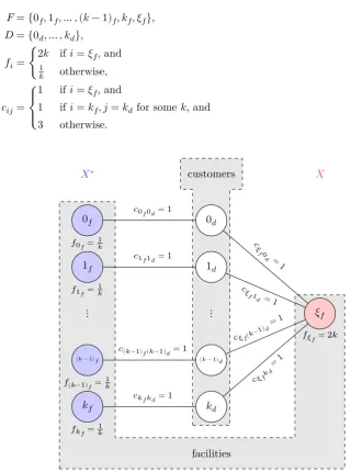
Proof. The following example, inspired by Arya et al. [3], proves the theorem (see also Figure 2). Choose a 𝑘 ∈ℕ, whose value will be specified later.

𝐹 = {0𝑓, 1𝑓, … , (𝑘 − 1)𝑓, 𝑘𝑓, 𝜉𝑓},

𝐷 = {0𝑑, … , 𝑘𝑑},

𝑓𝑖= {

2𝑘 if𝑖 = 𝜉𝑓, and

1

𝑘 otherwise,

𝑐𝑖𝑗=

⎧ { ⎨ { ⎩

1 if𝑖 = 𝜉𝑓, and

3 otherwise. facilities customers 0𝑓 1𝑓 ⋮

(𝑘 − 1)𝑓

𝑘𝑓 𝑓0𝑓=

1 𝑘

𝑓1𝑓=

1 𝑘

𝑓(𝑘−1)𝑓=

1 𝑘

𝑓𝑘𝑓=

1 𝑘

0𝑑

1𝑑

⋮

(𝑘 − 1)𝑑

𝑘𝑑

𝜉𝑓

𝑓𝜉𝑓= 2𝑘 𝑐0𝑓0𝑑= 1

𝑐1𝑓1𝑑= 1

𝑐_(𝑘−1)_𝑓_(𝑘−1)_𝑑= 1

𝑐_𝑘_𝑓_𝑘_𝑑= 1

𝑐_𝜉 𝑓₀

𝑑 ₌ 1

𝑐_𝜉 𝑓1_𝑑 _{= 1}

𝑐𝜉𝑓(𝑘−1) 𝑑

= 1

𝑐𝜉𝑓𝑘 𝑑

=1

[image:21.595.95.416.152.583.2]

𝑋∗ _𝑋

Figure 2: Example used in Theorem 12 (indirect service costs not shown)

The optimal solution 𝑋∗ _is _{0

𝑓, … , 𝑘𝑓}, with 𝑐(𝑋∗, 𝜎∗) = (𝑘 + 1)(1 + 1𝑘). This instance is 3𝑘

(𝑘+1)(1+1/𝑘)-perturbation resilient, as we will show by comparing all solutions𝑋 ≠ 𝑋

∗ with_𝑋∗ for all𝛾-perturbations(𝐹 , 𝐷, 𝑓′_{, 𝑐}′₎_{. By letting} _𝑘_{go to infinity, the perturbation resilience comes} arbitrarily close to 3, as required by the theorem.

Consider two cases: 𝜉𝑓∈ 𝑋and𝜉𝑓∉ 𝑋. For the first case, assume𝜉𝑓∈ 𝑋. If so,𝑐(𝑋, 𝜎) ≥ 3𝑘 + 1. Thus,𝑐′_(𝑋∗_{, 𝜎}∗_{) ≤ 3𝑘 < 3𝑘 + 1 ≤ 𝑐}′_{(𝑋, 𝜎)}_{, completing the first case.}

The second case is when𝜉𝑓∉ 𝑋. Without loss of generality, let𝑋 = {0𝑓, … , (|𝑋| − 1)𝑓}. Since

𝑐′

𝑖𝑓𝑖𝑑< 3 ≤ 𝑐 ′ 𝑖′_𝑖

𝑑 for𝑖 ∈ {0, … |𝑋| − 1}, 𝑖

′_{∈ 𝐹}_⧵_{𝑖

(22)

to the same facility in both𝑋∗ _and_𝑋_{, i.e.} _𝜎∗_(𝑖

𝑑) = 𝜎(𝑖𝑑) = 𝑖𝑓. For the other customers𝑗𝑑 with

𝑗 ∈ {|𝑋|, … , 𝑘}, look at the following quantity:

−𝑓′ 𝑗𝑓+ 𝑐

′

𝜎(𝑗𝑑)𝑗𝑑− 𝑐 ′ 𝜎∗_(𝑗

𝑑)𝑗𝑑≥ −

3

(𝑘 + 1)(1 +1_𝑘)+ 3 −

3𝑘 (𝑘 + 1)(1 +1_𝑘)

= 3 𝑘 + 1 > 0.

Using this quantity, it is possible to bound the difference between𝑐′_(𝑋∗_{, 𝜎}∗₎_and_𝑐′_{(𝑋, 𝜎)}_:

𝑐′_{(𝑋, 𝜎) − 𝑐}′_(𝑋∗_{, 𝜎}∗_{) =} 𝑘

∑

𝑗=|𝑋|

𝑐′

𝜎(𝑗𝑑)𝑗𝑑− 𝑐 ′ 𝜎∗_(𝑗

𝑑)𝑗𝑑− 𝑓 ′ 𝑗𝑓 > 0,

so𝑐′_(𝑋∗_{, 𝜎}∗_{) < 𝑐}′_{(𝑋, 𝜎)}_{, completing the second case.}

For both cases it holds that𝑐′_(𝑋∗_{, 𝜎}∗_{) < 𝑐}′_{(𝑋, 𝜎)}, for all solutions_{𝑋 ≠ 𝑋}∗, so instance_{(𝐹 , 𝐷, 𝑓, 𝑐)} is 3𝑘

(𝑘+1)(1+1/𝑘)-perturbation resilient. Also, 𝑋 = {𝜉𝑓} ≠ 𝑋

∗ is a local minimum, completing the proof.

Note that the example used in this theorem has a local minimum𝑋 = {𝜉𝑓}with cost𝑐(𝑋)which converges to3𝑐(𝑋∗₎_as_𝑘_{goes to infinity. This shows that the 3-approximation bound of local} search for FLP in general, as shown in Theorem 9, is tight.

3.2 Subsets of local minima

Knowing something about local minima, it is useful to relate other solutions to local minima. In the following theorem we show that solutions which are subsets of the local minima𝑋 can

always be augmented with extra facilities without increasing the solution’s cost. If the solution is a subset of the optimal solution𝑋∗_{for a} _𝛾_{-perturbation resilient instance, then any addition of} facilities in𝑋∗ _{but not in the solution will decrease the solution’s cost.}

Theorem 13.For all instances(𝐹 , 𝐷, 𝑓, 𝑐)of the FLP, with any possible local minimum(𝑋, 𝜎𝑋),

for all solutions𝑌, where𝑌is a strict subset of𝑋, the following holds:

• For any added facility𝑖 ∈ 𝑋⧵𝑌, the costs can only get lower, i.e. 𝑐(𝑌 ) ≥ 𝑐(𝑌 ∪ {𝑖}), and

• If 𝑐(𝑌 ) ≠ 𝑐(𝑋), at least one facility𝑖 ∈ 𝑋⧵𝑌has 𝑐(𝑌 ) > 𝑐(𝑌 ∪ {𝑖}).

Additionally, if the instance is 𝛾-perturbation resilient, all facilities 𝑖 ∈ 𝑋∗ _⧵_𝑌 _have _{𝑐(𝑌 ) >}

𝑐(𝑌 ∪ {𝑖}).

Proof. Because𝑋is a local minimum, dropping facility 𝑖 ∈ 𝑋⧵𝑌leads to equal or higher costs.

Thus

0 ≤ −𝑓𝑖+ ∑ 𝑗∈𝐷 𝜎𝑋(𝑗)=𝑖

min

𝑖′_∈𝑋_⧵_{𝑖}𝑐𝑖′𝑗− 𝑐𝑖𝑗 (5)

≤ −𝑓𝑖+ ∑ 𝑗∈𝐷 𝜎𝑋(𝑗)=𝑖

𝑐𝜎𝑌(𝑗)𝑗− 𝑐𝑖𝑗

≤ −𝑓𝑖+ ∑ 𝑗∈𝐷

max{𝑐𝜎𝑌(𝑗)𝑗− 𝑐𝑖𝑗, 0}

(23)

3. Local search

so𝑐(𝑌 ) ≥ 𝑐(𝑌 ∪ {𝑖}) for all 𝑖 ∈ 𝑋⧵𝑌, and𝑐(𝑌 ) > 𝑐(𝑌 ∪ {𝑖}) if𝑋 = 𝑋∗ _and_{(𝐹 , 𝐷, 𝑓, 𝑐)} _{is a}

𝛾-perturbation resilient instance, since inequality (5) is strict for𝛾-perturbation resilient instances

and optimal solution 𝑋∗_.

Now, assume𝑐(𝑌 ) ≠ 𝑐(𝑋)and define𝑔(𝑖) = −𝑓𝑖+ ∑𝑗∈𝐷,𝜎𝑋(𝑗)=𝑖𝑐𝜎(𝑗)𝑗− 𝑐𝑖𝑗. Because of the above inequalities,0 ≤ 𝑔(𝑖) ≤ 𝑐(𝑌 ) − 𝑐(𝑌 ∪ {𝑖})for all facilities𝑖 ∈ 𝑋⧵𝑌. Combining this for all such

facilities:

∑

𝑖∈𝑋⧵𝑌

𝑔(𝑖) = − ∑

𝑖∈𝑋⧵𝑌

𝑓𝑖+ ∑ 𝑗∈𝐷 𝜎𝑌(𝑗)∈𝑋⧵𝑌

𝑐𝜎𝑌(𝑗)𝑗− 𝑐𝜎𝑋(𝑗)𝑗

= − ∑

𝑖∈𝑋⧵𝑌

𝑓𝑖+ ∑ 𝑗∈𝐷

𝑐𝜎𝑌(𝑗)𝑗− 𝑐𝜎𝑋(𝑗)𝑗

= 𝑐(𝑌 ) − 𝑐(𝑋) > 0.

So at least one 𝑖 ∈ 𝑋⧵𝑌has𝑔(𝑖) > 0and thus𝑐(𝑌 ) > 𝑐(𝑌 ∪ {𝑖}).

(24)

(25)

4. Greedy algorithms

4 Greedy algorithms

In this section we will consider several greedy algorithms for𝛾-perturbation resilient instances.

Greedy algorithms have the advantage of being efficient but they do not always give the optimal solution to an instance. The chosen greedy algorithms, greedy facility addition and greedy facility deletion, are an obvious choice for a greedy FLP algorithm because of their simplicity. These generally do not result in the optimal solution for the FLP, and we will show that this remains true for the𝛾-perturbation resilient FLP, even for high𝛾.

4.1 Greedy facility addition

One of the simplest greedy algorithms is greedy facility addition. In this algorithm, you start from some initial set of facilities𝑋(potentially empty) and greedily add facilities until some condition is

met. Here, we add the facility with maximum cost reduction (i.e.−𝑓𝑖+ ∑𝑗∈𝐷max{𝑐𝜎(𝑗)𝑗− 𝑐𝑖𝑗, 0}), as long as that remains positive. This greedy algorithm seems promising, based on the results of Theorem 13.

The following(7₂− 𝜀)-perturbation resilient FLP instance is a counterexample that shows this

does not always yield the optimal solution:

𝐹 = {1𝑓, 2𝑓, 3𝑓, 4𝑓},

𝐷 = {1𝑑, 2𝑑, 3𝑑},

𝑓 = (0, 0, 0, 1) ,

𝑐 =⎛⎜⎜_⎜

⎝

1 50 50 52 1 7 52 7 1 54 3 3

⎞ ⎟ ⎟ ⎟ ⎠ ,

𝑋 = {1𝑓},

𝑋∗_{= {1}

𝑓, 2𝑓, 3𝑓}.

1𝑓 2𝑓 3𝑓 4𝑓 1𝑑 2𝑑 3𝑑 𝑐₁_𝑓₁_𝑑= 1

𝑐1𝑓2𝑑 = 50

𝑐₁ 𝑓3_𝑑

= 50

𝑐2𝑓2𝑑= 1

𝑐3𝑓3𝑑= 1 𝑐₄

𝑓2_𝑑

= 3

𝑐4𝑓3𝑑 = 3 𝑓1𝑓= 0

𝑓2𝑓= 0

𝑓3𝑓= 0 𝑓4𝑓= 1

Figure 3: Counterexample to greedy facility addition (indirect service costs not shown)

In this example, the optimal solution is𝑋∗_{= {1}

(26)

facility addition does not yield𝑋∗ _{with this example, we start from} _{𝑋 = {1}

𝑓}. This may not seem reasonable, but just adding a lot of copies of customer1𝑑to the example makes this a good choice when starting from the empty set. In the next step, several facilities can be added, with the following cost reduction:

𝑐({1𝑓}) − 𝑐({1𝑓, 2𝑓}) = 92,

𝑐({1𝑓}) − 𝑐({1𝑓, 3𝑓}) = 92,

𝑐({1𝑓}) − 𝑐({1𝑓, 4𝑓}) = 93.

So the greedy algorithm chooses to open facility4𝑓and update𝑋to{1𝑓, 4𝑓}, even though this is not optimal.

The example is (7₂ − 𝜀)-perturbation resilient, as switching from the optimal solution 𝑋∗ ₌

{1𝑓, 2𝑓, 3𝑓} only starts making sense once both customer 2𝑑 and 3𝑑 switching to facility 4𝑓 is advantageous enough, which happens when you have a 7

2-perturbation of this example.

4.2 Greedy facility deletion

Another greedy algorithm is greedy facility deletion. In this algorithm, you start from some initial set of facilities𝑋, e.g.𝑋 = 𝐹, and greedily drop facilities until some condition is met. Here, we

drop the facility with maximum cost reduction (i.e.𝑓𝑖+ ∑𝑗∈𝐷𝑐𝜎(𝑗)𝑗− min𝑖′_∈𝑋_⧵_{𝑖}𝑐_𝑖′𝑗), as long as that remains positive.

The following FLP instance, using 𝑘 ∈ ℕ, 𝑘 ≥ 4, is a counterexample that shows this does

not always yield the optimal solution. When𝑘converges to infinity, the instance converges to

3-perturbation resilience.

𝐹 = {0𝑓, 1𝑓, … , 𝑘𝑓},

𝐷 = {1𝑑, … , 𝑘𝑑},

𝑓𝑖=

⎧ { ⎨ { ⎩

3𝑘 − 2

𝑘 − 2 if𝑖 = 0𝑓, and 3𝑘 − 3

𝑘 − 2 otherwise,

𝑐𝑖𝑗=

⎧ { ⎨ { ⎩

1 if𝑖 = 0𝑓, and

3 otherwise, 𝑋∗_{= {0}

𝑓}.

The optimal solution is 𝑋∗ _{= {0}

𝑓}, since opening less facilities always reduces 𝑐𝐹(𝑋)in this example, and letting0𝑓stay open makes sure that the service costs𝑐𝑆(𝑋∗)stay minimal. However, greedy facility deletion, when starting with𝑋 = 𝐹, drops facility0𝑓first. This is because it is the most expensive facility and the service costs do not increase in the first deletion, no matter which facility in𝑋you close.

(27)

5. Relation to approximation algorithms

5 Relation to approximation algorithms

In this section we will show one of the best approximation algorithms for the FLP, the Jain-Mahdian-Saberi algorithm [17], with approximation ratio 1.61. As approximation algorithms guarantee a solution𝑋 with cost𝑐(𝑋) ≤ 𝛼𝑐(𝑋∗₎_{, with}_𝛼_{depending on the algorithm, it seems} obvious that these algorithms should give the optimal solution to𝛾-perturbation resilient instances,

if 𝛾 ≥ 𝛼. After all, with 𝛾-perturbation resilience you can multiply the costs of the optimal

solution with𝛾and it is still the optimal solution. We will show that this conjecture is not true,

even for a good algorithm like the Jain-Mahdian-Saberi algorithm.

5.1 The Jain-Mahdian-Saberi algorithm

To understand the Jain-Mahdian-Saberi algorithm, it is useful to first look at the integer linear program (LP) formulation of the facility location problem:

min ∑

𝑖∈𝐹

𝑓𝑖𝑦𝑖+ ∑ 𝑖∈𝐹

∑

𝑗∈𝐷

𝑐𝑖𝑗𝑥𝑖𝑗

s.t. 𝑥𝑖𝑗≤ 𝑦𝑖 for all𝑖 ∈ 𝐹 , 𝑗 ∈ 𝐷,

∑

𝑖∈𝐹

𝑥𝑖𝑗= 1 for all𝑗 ∈ 𝐷,

𝑥𝑖𝑗∈ {0, 1} for all𝑖 ∈ 𝐹 , 𝑗 ∈ 𝐷,

𝑦𝑖∈ {0, 1} for all𝑖 ∈ 𝐹.

Of course, solving this LP is not simpler than solving the FLP. But if you relax the integer variables such that𝑥𝑖𝑗∈ [0, 1] and𝑦𝑖∈ [0, 1], it is possible to solve the LP in polynomial time. This is the basis of LP-rounding algorithms, which calculate a FLP solution from the relaxed LP solution, which typically is not an integer solution. Better algorithms can be derived by also using the dual of the relaxed LP and the resulting complementary slackness. These algorithms are called primal-dual algorithms. Of course, the difficulty in this process is somehow getting a integral solution.

Definition. The Jain-Mahdian-Saberi algorithm[17] is a primal-dual algorithm for the FLP. For every customer 𝑗and facility 𝑖, variables𝑤𝑖𝑗 and𝑣𝑗 are introduced. Every customer starts unconnected and every facility starts closed. The algorithm starts by maintaining 𝑣𝑗= 𝑡 and

processes the following events while increasing𝑡:

• 𝑣𝑗= 𝑐𝑖𝑗 for some unconnected customer 𝑗and closed facility 𝑖. Start increasing𝑤𝑖𝑗 such

that 𝑐𝑖𝑗+ 𝑤𝑖𝑗= 𝑣𝑗.

• ∑_𝑗∈𝐷𝑤𝑖𝑗 = 𝑓𝑖 for some closed facility 𝑖. Open facility 𝑖 and, for all customers 𝑗 with

𝑤𝑖𝑗> 0, stop increasing𝑣𝑗and set𝑤𝑖′_𝑗= max{0, 𝑐_𝑖𝑗− 𝑐_𝑖′_𝑗}for all𝑖′∈ 𝐹and mark customer

𝑗as connected.

• 𝑣𝑗= 𝑐𝑖𝑗 for some unconnected customer 𝑗 and open facility𝑖. Stop increasing 𝑣𝑗 and set

𝑤𝑖′_𝑗= max{0, 𝑐_𝑖𝑗− 𝑐_𝑖′_𝑗} for all 𝑖′∈ 𝐹and mark customer 𝑗 as connected.

Ties between events, when occurring at the same 𝑡, are broken arbitrarily. When there are no

more events to be processed, the algorithm will have connected all customers and yields a set of open facilities.

(28)

factor-revealing LP [17]. Examples of these guarantees are(𝛼 = 1, 𝛽 = 2), (𝛼 = 1.11, 𝛽 = 1.78)

and(𝛼 = 1.61, 𝛽 = 1.61). This means that the solution of the Jain-Mahdian-Saberi algorithm

satisfiesall of these guarantees, you do not have to choose.

Note that better algorithms exist for the FLP (e.g. the 1.5-approximation algorithm by Byrka and Aardal [10]) and that the difference in approximation guarantee for the service costs𝑐𝑆(𝑋∗) and facility costs𝑐𝐹(𝑋∗)can be exploited to yield better approximation ratios (see Charikar and Guha [11], yielding a ratio of 1.51 when used with the Jain-Mahdian-Saberi algorithm).

5.2 Perturbation resilience and solutions of approximation algorithms

Since the 𝛾-perturbation resilience property is almost equivalent to saying that the optimal

solution stays unique and optimal even when its costs are multiplied by𝛾, it seems there must

be some kind of relation to approximation algorithms for the FLP. After all, if some calculated solution cannot be worse than𝛼times the optimum, then it likely must imply that it either is

equal to the optimum or, if not, that𝛾 < 𝛼, for𝛾-perturbation resilient instances. This reasoning

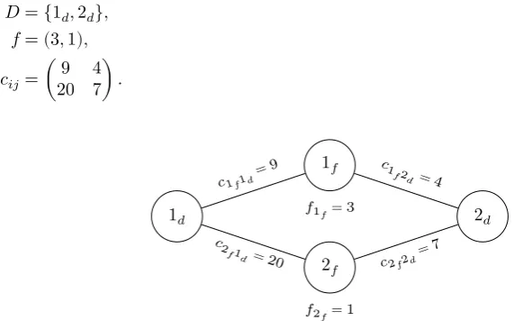
is wrong however, as we will show with the following example. Define the following instance (see Figure 4):

𝐹 = {1𝑓, 2𝑓},

𝐷 = {1𝑑, 2𝑑},

𝑓 = (3, 1),

𝑐𝑖𝑗= (

9 4 20 7) .

1𝑓

2𝑓

1𝑑 2𝑑

𝑐1𝑓1𝑑

= 9 𝑐1_𝑓₂

𝑑= 4

𝑐₂ 𝑓1_𝑑 _{= 20}

𝑐2𝑓2𝑑 = 7 𝑓1𝑓= 3

[image:28.595.132.418.352.530.2]

𝑓2𝑓= 1

Figure 4: An𝛼-perturbation resilient instance which has an𝛼-approximate solution𝑋 ≠ 𝑋∗

This example has (7₄− 𝜀)-perturbation resilience. This can be seen by considering the cost of

all solutions under the𝛾-perturbation defined in Theorem 5, where the following costs already

assume that𝛾 < 7₄:

𝑐′_(𝑋∗_{) = 𝑐}′_({1

𝑓}) = 16𝛾,

𝑐′_({2

𝑓}) = 28,

𝑐′_({2

𝑓, 3𝑓}) = 1 + 16𝛾.

So𝑐′_(𝑋∗_{) < 𝑐}′_(𝑋) for all solutions _{𝑋 ≠ 𝑋}∗ iff _{𝛾 <} 7

4, so the instance is ( 7

4− 𝜀)-perturbation resilient.

The Jain-Mahdian-Saberi algorithm has an approximation ratio of 1.61, which is smaller than 7

(29)

5. Relation to approximation algorithms

𝑋 = {1𝑓, 2𝑓} ≠ 𝑋∗. So this example shows that𝛼-approximation algorithms do not guarantee optimal solutions for𝛾-perturbation resilient instances with𝛾 ≥ 𝛼.

(30)

Perturbation resilience for the facility location problem