Parallel magnetic particle imaging: compressed sensing of field free line excitations

(1)

1

Parallel magnetic particle imaging:

compressed sensing of field free line

excitations

Normen Oude Booijink

MSc. Thesis

October 2016

(2)

Abstract

We developed a speed versus quality improvement of the currently most promising imaging modality that images superparamagnetic nanoparticles that are injected into a body: Magnetic Particle Imaging (MPI). We design a more informative hardware setup, that uses multiple receive channels similar to the setup in parallel Magnetic Resonance Imaging (MRI). To process the simulated data from these parallel coils, we use convex optimization reconstruction algorithms that can combine the extra information to find either the same image quality at shorter scan time, or improve image quality at the same scan time. To get the speed improvement, we decrease the number of projections in field free line MPI, so that Fourier space is undersampled. The idea for this was inspired by results from Magnetic Resonance Imaging, and the Fourier Slice Theorem. This motivated us to be the first to prove that the concept of parallel imaging can be applied to MPI.

(3)

1 Acknowledgements

(5)

2 Introduction

Magnetic Particle Imaging (MPI) is a relatively young imaging modality, that aims to image the density dis-tribution of a magnetic tracer in a body. One could say that MPI is currently in the state where Magnetic Resonance Imaging (MRI) was in the 1980s and 90s: the concept works and (animal) scanners have been built. Back then people tried to mathematically optimize excitation strategies for MRI, for example using control theory. Also, mathematics was used to extract more information from a scan, by optimizing over hardware setups and scanning trajectories [34],[35],[39]. The latter are called compressed sensing and parallel imaging techniques, and have inspired this thesis. We argue that there are similar opportunities for MPI, as the hardware of MPI has similarities with MRI. But let us first motivate why MPI is an imaging modality worth spending time on in the first place.

The use of magnetic nanoparticles in medicine was first investigated during the end of the 20th century, and started to take serious forms in the 2000s as people started to see competitive advantages over some of the es-tablished techniques, such as improvements in contrast and patient safety in imaging applications, and accurate drug delivery through magnetic targeting [1],[2],[3], [4], [5] [6]. Also more recently, several applications have been presented that use the size and magnetic properties of certain nanoparticles [6], [7],[8],[9],[10]. Regarding medical imaging techniques, the most promising of these applications is Magnetic Particle Imaging (MPI). The modality was invented during the years 2000 and 2001 by Jurgen Weizenecker and Bernard Gleich [11], both working for the Philips Research Laboratory in Hamburg, Germany. The physical principles along with some first experiments were published in the journal Nature by these two researchers in 2005 [7]. The concept of MPI relies on the nonlinear magnetization curve of superparamagnetic iron oxide nanoparticles (SPIONs). Because of their size - only a few atoms wide - the SPIONS are very suitable for injection into the human body and can penetrate through lots of different tissues. The body is then placed in a scanner that uses a smart hardware setup mostly consisting of coils, to image the nanoparticle distribution in the body. A more detailed description of the exact functioning of an MPI scanner and how the image is formed are given in sections 3.2 and 3.3. With this knowledge, we investigate how both the hardware and the reconstruction should be redesigned to make parallel MPI feasible.

The big competitive advantage of MPI is its contrast performance in combination with patient safety. Contrast agents and tracers in medical imaging are present in almost every medical imaging technique as they provide visualization of structures that can not be seen without, and are crucial for many diagnoses. But most of the current contrast agents like iodine in X-ray, can not be used for the imaging of Chronic Kidney Disease (CKD) patients, which is a very large group [12]. And in PET and SPECT scans, the radioactive tracers yield safety and logistic problems for both the patient and the medical personnel. Importantly, the iron oxide nanoparticles used in MPI are not radioactive and are processed in the liver, so they don´t affect the kidneys. The only other current imaging modality where SPIONs are used as a contrast agent is MRI, but it is suboptimal because the background signal from the host tissue is a limiting factor with respect to image contrast [13],[14]. MPI aims to only measure the signal that emanates from the injected magnetic tracer, and it does so by taking advantage of the nonlinear magnetization curve of SPIONs. By analyzing the higher harmonics of the signal that emanates from the nonlinear response of these SPIONs to an exciting magnetic field, the signal due to the SPIONs can be extracted from the entire inductively received signal. This yields an image that results from a signal that is not distorted by signals from the hosting tissue or the exciting magnetic field. Therefore, very high contrast can be obtained via this imaging modality. In order to compete with other imaging modalities, future research on MPI will have to focus on resolution enhancement, speed and new applications. Room for improvement can mainly be found in the hardware of MPI scanners, the image reconstruction process and the design of the nanoparticles. The speed improvement presented in this thesis will mainly focus on a change in the reconstruction approach, that also implies a new hardware setup.

(6)

in Berkeley and focused on their method, but our parallel imaging model can also easily be applied to the system matrix approach.

3 Parallel Imaging and MPI physics

In this section we will first describe what parallel imaging is, and why it is useful. Then, we explore the possibilities for parallel imaging in MPI.

3.1 Parallel imaging

In parallel imaging, multiple receive channels are used to pick up a certain signal, where the spatial location of these receive channels is exploited to extract extra information. This extra information can either be used to improve image quality, or to allow for less data acquisition leading to shorter scanning times. For example, in parallel MRI, multiple images m1, m2, ..., mL are obtained due to the presence of Ldifferent receive coils.

[image:6.595.177.418.357.549.2]

These images can then be combined into the desired final image m by defining a good forward model, that can be inverted directly or solved algorithmically, dependent on the complexity of the scanning procedure. A good reference for a historical overview of the different algorithms and methods that use parallel imaging to increase MRI performance is [32]. The most important reconstruction algorithms are SMASH [34], SENSE [35], GRAPPA [36] and (E)SPIRiT [37],[38]. SENSE and ESPIRiT are the best option in our opinion, since they aim to fully reconstruct the actual image m(x, y), whereas SMASH and GRAPPA aim to compute an approximation. We now give two examples form MRI, to illustrate the power of parallel imaging. The first example gives a good intuition as to why the power of parallel imaging comes from the extra spatial information. The second example is more general, and will be very useful for our approach to parallel MPI.

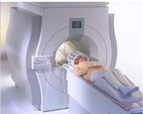
Figure 1: Parallel MRI in practice. In this photo, an MRI of the brain is made using 12 parallel receive coils.

First example (Cartesian MRI)

Assume that we aim to reconstruct an image that contains density information m(x) at voxelsxp, wherepis

an index that runs over the number of voxels. Each receive channelCi has a spatially variant sensitivity map

Si(x), yielding images

mi(x) =Si(x)m(x)

after an MRI scan. So, for a particular voxelp, we have

    

m1(xp)

m2(xp)

.. .

mL(xp)

     | {z }

ms

=

    

S1(xp)

S2(xp)

.. .

SL(xp)

     | {z }

C

m(xp) (1)

and we can solve

m(xp) = S⊥S

−1

(7)

for each voxel, to obtain the desired density image m(x). Now, the power of parallel imaging lies in the acceleration of scanning times in MRI. In Cartesian sampling trajectories, the scan time is dictated by the number of phase encodes, as usually only one phase encode is done within every time repetition (TR). So, if one would divide the number of phase encodes byR, entire MRI scanning time will reduce by a factorR. In our example of Cartesian parallel MR imaging with undersampling factorR, the phase encode is in thex-direction, so we put zeros on the horizontal lines in k-space we have not sampled. Then, we compute the inverse Fourier transform to yield an aliased image (due to the increase in ∆ky and thus decrease in FOVy). Also, for each

voxel xp in the aliased image, one backtracks the R‘source voxels’ in the actual image that have contributed

to the aliasing in voxel xp. Call these source voxelsx1p,x2p, ...,xRp. Then, for each voxelxp we can solve the

system     

m1(xp)

m2(xp)

.. .

mL(xp)

     | {z }

ms =     

S1(x1p) S1(x2p) · · · S1(xRp)

S2(x1p) S2(x2p) · · · S2(xRp)

..

. ... . .. ...

SL(x1p) SL(x2p) · · · SL(xRp)

    

| {z }

C     

m(x1p)

m(x2p)

.. .

m(xRp)

     | {z }

m(xp)

(3)

which has solution

m(xp) = S⊥S

−1

S⊥ms. (4)

So we see that we obtain the density values for R voxels of the actual image using a system with sizeL×R. An example of parallel imaging results for an 8 coil system is given in figures 2 and 3 . We see that the system does quite a good job at reconstructing the original brain image while we undersample by a factor of R= 2. Important to note, is that undersampling in MRI occurs in Fourier-space. Due to the undersampling, less information is obtained, but not all information is lost. One needs to be careful with this; there is only room for undersampling when it doesn’t directly delete too much information you need to fill all the pixels in the image with the right density. We will see that this forms a problem in standard MPI.

(a)

[image:7.595.120.473.400.530.2]

(b)

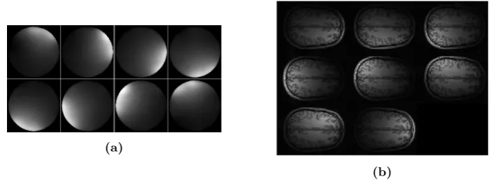
Figure 2: (a)Estimates for the sensitivity maps of eight coils used for parallel MR imaging of the brain.(b)

The resulting eight MR images of a brain slice when sampling at the Nyquist rate.

(a) (b)

Figure 3: (a): The 8 coil images reconstructed from undersampled data: a factor R = 2 in the y-direction. Note the increased signal intensity at aliased pixels. (b): Corresponding parallel imaging reconstruction using SENSE.

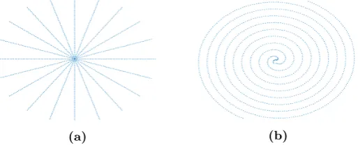
[image:7.595.127.472.586.715.2]

(8)

In MRI, other sampling trajectories than Cartesian can be favorable in terms of scanning times and signal in-formation. Spiral and radial trajectories for example, collect more data at the center of k-space, which contains most of the information. An other example is random sampling, which is favorable for compressed sensing [39].

Parallel imaging can again be used to get good quality images while k-space is being undersampled

[image:8.595.170.427.133.237.2]

non-(a) (b)

Figure 4: Two non-Cartesian sampling trajectories in MRI. We will see that trajectory (a) is the key to parallel MPI.

uniformly. Two of these sampling trajectories are given in figure 4. Unfortunately, in these situations it is impossible to backtrack which pixels contributed to the aliasing in each coil image like we did in the first exam-ple. Hence, the reconstruction approach from the previous example doesn’t apply anymore, because basically any pixel could have contributed to the aliasing and the matrix C would become too big and impossible to form. Therefore, a forward model is derived and the corresponding inverse problem is solved iteratively through an algorithm. The forward model looks like

Eρ=d (5)

(9)

[image:9.595.150.445.54.342.2]

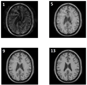
Figure 5: Iterative SENSE reconstruction using the conjugate gradient method. The reconstructions after the 1st, 5th, 9th and 13th iteration are shown.

3.1.1 Checklist for parallel imaging

In the previous section, we saw that parallel imaging can be used to decrease scan times in MRI. This is possible because MRI suffices to three key requirements that we identified. To obtain shorter scanning times using parallel imaging, a medical imaging technique has to suffice to:

1. It is possible to measure the signal at different locations. Multiple receive channels with different sensitivities to signals can only be realized if the signal can be detected from different locations around the object. An imaging technique that fails this condition is X-ray CT ; the signal that is being measured is just an attenuation of the original beam, that only goes in one direction. Hence, the only location of the detector that makes sense, is on the opposite side of the transmitter. Therefore, parallel imaging is not suitable for X-ray CT.

2. There is room for undersampling while still scanning each location of the object Undersam-pling, i.e. obtaining less data, is only desirable if the whole object can still be reconstructed. That is why data acquisition in k-space is so powerful, because each data point in k-space could reflect information from any location in the object. There might still be enough information in a subset of the k-space data to reconstruct the whole object.

3. Except for sensitivity differences, each receive channel has to receive the same signal. If the data from two receive channels reflect fundamentally different physics, these data can not be combined, and parallel imaging makes no sense anymore.

In the next subsections, we will explore if MPI in its standard form suffices to these requirements, and if not, which hardware adjustments we have to make.

3.2 Physical principles of MPI

(10)

[image:10.595.190.402.123.299.2]

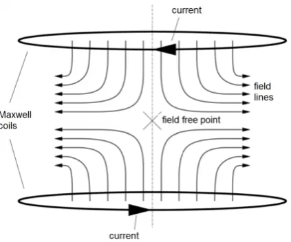
A beautiful part of the MPI technique is the way Weizenecker and Gleich determine where each part of the received signal, which is just a time series, came from in space. First, a body is subjected to a strong gradient field generated by opposing maxwell coils, which is also referred to as the gradient field. In this gradient field, a field free point (FFP) is present. An illustration of this is given in figure 6.

Figure 6: The gradient field produced by two opposite Maxwell coils contains a field free point (FFP).

To magnetically saturate all magnetic material outside the FFP, the gradient field generated by the Maxwell coils is chosen to be about 3 to 6 Tm−1 _{in strength. In such a strong field, all magnetic material is saturated}

except for the magnetic material inside the FFP. In the absence of a magnetic field, a population of SPIONs has zero magnetic moment: as each individual SPION’s magnetic moment is randomly oriented due to thermal agitation, their magnetic moments cancel out yielding zero magnetization for an ensemble of these particles. So after the gradient field is turned on, only the particles in the FFP are randomly aligned. Now comes the crucial part: a spatially homogeneous magnetic field is added, causing the FFP to shift to another position. The particles that were at the previous location of the FFP will now all align their magnetic moments with the gradient field, causing a change of magnetic flux through the receive coils that we can register, and know to have originated from the FFP. The amplitude of the signal then holds information about the the nanoparticle density at that location.

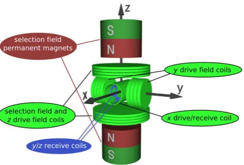
So two more kinds of hardware are needed: Drive field coils, which generate the additional homogeneous magnetic field, and receive coils that register the response of the nanoparticles in the FFP. Two type of drive field coils are present. The first one is the exciting drive field, that rapidly changes it’s amplitude so that the FFP also shifts rapidly, causing a sudden change in magnetization of the SPIONs. The second type of drive field coil creates a field called the bias field that is similar to the drive field but changes it’s amplitude relatively slow, over a bigger range. In this way, the bias field aims to slowly move the FFP over the body so that the whole body is being scanned. A schematic setup of a three-dimensional MPI scanner as proposed by Weizenecker and Gleich [15] is given in figure 7. The German group has a slightly different nomenclature: the gradient fields are called selection fields.

(11)

[image:11.595.181.419.55.216.2]

Figure 7: Schematic setup of a 3-D MPI scanner as proposed by the Philips research group in Hamburg. Note that the selection field is what we call the gradient field.

3.3 Reconstruction approaches in MPI

The goal of the MPI reconstruction process is to find the exact spatial distribution of the SPIONs over the body, including quantitative density information. In medical imaging, the region of interest in the body is often referred to as field of view (FOV). The FFP has to be moved over the entire FOV to obtain the spatial density distribution of the SPIONs, recording a signal at each time step to form a discrete image. As mentioned in the previous section, we don’t have to move the body to move the FFP’s relative position. Magnetic fields add, so every contribution by the homogeneous drive fields and bias fields will shift the location of the FFP created by the gradient field. By building the drive field coils in each of the three Cartesian directions, the FFP can be moved over 3-D space in any way that is desirable. The drive field rapidly shifts the FFP and causes a rapid change in magnetization of the SPIONs. In addition, the bias field slowly moves the FFP over the entire FOV. The change in magnetization is recorded by a receive coil, forming the datad. Currently there are two approaches to reconstructing an MPI image fromd: system matrix MPI and x-space MPI.

3.3.1 System matrix MPI

This reconstruction method was initiated by Weizenecker and Gleich, and later adapted by several researchers, mostly active in Germany [7] [16] [17]. The conventional model assumes a linear connection between the particle density ρ(x) and the MPI signal s(t). The system matrixGencodes which coefficient should be used in this relationship:

s(t) =

Z

G(x, t)ρ(x)dx, t∈[ts, te], (6)

where ts andte denote the start and end time of the MPI scan, respectively. G indirectly contains all

infor-mation hidden in the MPI system and scanning trajectory: at each location of the FFP in thecalibration scan

on a phantom with unit concentration, the receive coils register a signal that originated from the FFP. But, even though the particle density is equal over the entire FOV, the geometry of the scanning procedure causes a variation of amplitudes in the signal. More on this can be read in the discussion section of [19]. When the actual scan on a phantom with unknown particle density distribution is done, the scanning procedure needs to be exactly as in the calibration scan. Then, the obtained data s and the system matrix G can be used to compute ρ(x). In the papers by Gleich and Weizenecker, this is done using direct inversion methods like Singular Value Decomposition on equation (1) [16].

A big disadvantage of the system-matrix approach is the time-consuming calibration scan. In [20], it took 6 hours to scan a 34x20x28 3D grid. Moreover, this calibration is only valid for a specific FOV and scanning trajectory. Changes in the setup would need a new calibration scan. But, from about 2009 up to now, the researchers from the Philips group try to fix this problem by theoretically deriving the system matrix [18],[19]. If this can be done accurately, there is no need for a physical calibration to obtain G.

3.3.2 x-space MPI

(12)

density at the location of the FFP at timetk. So the first papers on x-space MPI are all about the physics that

ultimately lead to the received signals. In [21], the first complete x-space model is given for 1-D signals. The location of the FFP can explicitly be given by setting the total magnetic field equal to zero. In 1-D, this yields

H(x, t) =H0(t)−G·x= 0.

Note that the drive fieldH0is only time-dependent, and the gradient fieldG·xis space dependent.The gradient G was conveniently chosen with a negative sign. The total magnetic field expressed as a function of space, time and the FFP is thus

H(x, t) =G· x−xs(t)

, (7)

wherexs(t) denotes the location of the FFP as a function of time. As said before, the MPI signal is the result of

the change in magnetic fluxφthrough the receive coils. This change is due to the change in total magnetization

M of the nanoparticles. In the 1-dimensional case, we get

s(t) =B1

d

dtφ(t) =B1 d dt

Z

M(x, t) dx. (8)

WhereB1[T /A] is just a constant that models the sensitivity of the receive coil. Langevin theory [23] is used to describe the magnetization of a SPION as a function of the applied magnetic field that they are subject to. The magnitude of the magnetization can be seen as the amount of atomic dipoles in the SPION molecules that are aligned with the applied magnetic field. If all atomic dipoles are aligned, we call it magnetically saturated. Langevin theory claims that the magnetization at a single pointxin a magnetic fieldH is

M(H) =mρ(x)L(kH). (9)

m is the magnetic moment of a nanoparticle [A·m−2_],_ρ_{is the nanoparticle density [kg}_·_m−3_{] and}

k= µ0m

kBT

.

Where µ0 is the vacuum permeability, kB is Boltzmann’s constant and T is the temperature. The Langevin

function

L(x) = coth(x)−1 x

is depicted in figure 8a. Note that it’s extreme values are -1 and 1, which is what we would expect from equation (9). With this knowledge, we can combine equations (7),(8) and (9) to obtain

s(t) =B1mρ(x)∗L˙(kG·x)

_x₌_x

s(t)

kG·x˙s(t). (10)

So, ignoring the constants involved, the received signalsat a time instanttk of a 1-D MPI scan is the result of

a convolution of the nanoparticle density in the FFP at time tk with the derivative of the Langevin function,

mulitplied by the FFP velocity. In [22], the above result is derived for the multidimensional case. There are

(a) The langevin function L de-scribes the magnetization of SPI-ONs as a function of the externally applied magnetic field.

(b) The point spread function in 1-D MPI is the derivative of the Langevin function.

(13)

Multi-dimensional x-space MPI

In [22], the researchers from the Berkeley Imaging Systems Laboratory write a multi-dimensional follow-up to the 1-D paper [21]. A gradient field in three dimensions with a FFP can be realized by H=Gx, with

G=

 

Gxx 0 0

0 Gyy 0

0 0 Gzz

 =Gzz

 

−1

2 0 0

0 −1

2 0

0 0 1

 ,

where Gzz is typically chosen such that µ0Gzz ≈ 2.4 to 6 T/m. To move the FFP over the 3-D volume, an

additional homogeneous but time-varying field Hs(t) = [Hx(t), Hy(t), Hz(t)] is added to the gradient field.

GivingGzz a convenient negative sign, the total field is

H(x, t) =Hs(t)−Gx,

so that the location of the FFP is

xs(t) =G−1Hs(t). (11)

In 3-D, there are more degrees of freedom w.r.t the excitation direction and the receive coil geometries. There-fore, the derived PSFh(x)is a 3×3 matrix with a function of (x, y, z) at each entry:

h(x)= ˙L(||Gx||/Hsat)

Gx

||Gx||

_Gx

||Gx||

T

G

+L(||Gx||/Hsat)

||Gx||/Hsat

I− Gx ||Gx||

_Gx

||Gx||

T!

G, (12)

whereLdenotes the langevin function as in section 3.3.2. An explicit PSF in scalar functional form is obtained once a scanning direction ˆ˙xsof the FFP is chosen:

h(x) =xc·h(x)xˆ˙s, (13)

where xc is the receive coil vector. Note that we useˆto indicate a normalized vector. Similar to the 1-D case,

the blurred MPI image results from a convolution with the PSF:

˜

ρ(x) = s(t)

||x˙|| =

B1(x)m

Hsat

ρ(x)∗ ∗ ∗xc·h(x)xˆ˙

_x₌_x

s(t)

, (14)

where B1(x) is the receive coil sensitivity. We will omit the term B1(x)m

Hsat in most of the calculations in this

report, for notation purposes. To give the reader some more intuition and visual support, we will shortly elaborate on the 2-D MPI PSF. Also, a good understanding of the PSF was crucial to the design of our parallel MPI approach.

Image resolution and the point spread function

In the world of imaging research, there are a lot of different measures for resolution [24]. In medical imaging, the measure that is mostly used is the full-width at half maximum of the point spread function of the imaging system. So in order to determine or enhance the resolution of a medical imaging technique, the point spread function must be understood in detail. For us, knowledge of the PSF will turn out to be crucial to prove that parallel MPI is possible. So let’s look at the details of the PSF for the 2-D case. Recall from equation (12) that for multidimensional MPI, the PSF is a tensor, that turns into a scalar PSF as soon as one picks an excitation (drive field coil) direction and a listening (receive coil) direction. Hence, the resolution in MPI will depend heavily on the choice for these two directions. After some math, one obtains from (12) that the 2D tensor PSF in the xy-plane is

h(x)=ET(x)·

G x2₊_y2

x2 xy −yx −y2

(15)

+EN(x)

G 0

0 −G

− G

x2₊_y2

x2 _xy

−yx −y2

, (16)

where we assumed a gradient field of

Gx= G 0 0 −G x y , (17) and set

ET(x) := ˙L(||Gx||/Hsat), (18)

EN(x) :=

L(||Gx||/Hsat)

||Gx||/Hsat

(14)

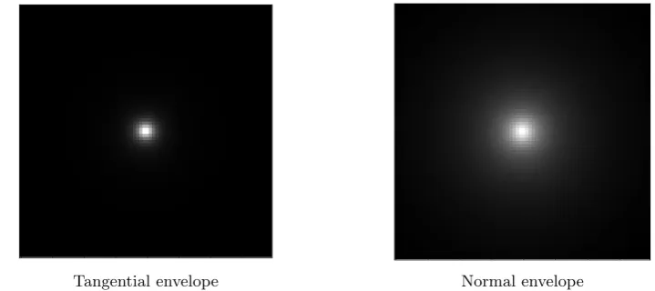
to be the tangential and normal envelopes of the PSF respectively. The tangential envelope and normal envelope of the MPI PSF represent different physics. The tangential envelope (good resolution) represents the change in magnitude of the magnetization, while the normal envelope represents change in magnetization due to rotation of the magnetic moments (bad resolution). In figure 9, these two envelopes are shown. To see how these two

[image:14.595.114.474.116.276.2]

Tangential envelope Normal envelope

Figure 9: The tangential envelope and normal envelope of the MPI multi-D PSF represent different physics. The tangential envelope (good resolution) represents the change in magnitude of the magnetization, while the normal envelope represents change in magnetization due to rotation of the magnetic moments (bad resolution).

envelopes affect the final scalar MPI PSF, choose the excitation vector ˆ˙xs and receive coil vector xc. Then,

according to equation (13)

h(x) =

1 0

h(x)

1 0

= Gx

2

x2₊_y2ET(x) +

G− Gx

2

x2₊_y2

EN(x)

=⇒ h(x)/G= x 2

x2₊_y2ET(x) +

y2

x2₊_y2EN(x).

[image:14.595.65.536.491.604.2]

In figure 10, we show this expression in terms of 2-D images. The resolution of the PSF is the best in the excitation direction, because the ’bad’ normal envelope is suppressed in that direction.

Figure 10: Visual representation of the different components of the point spread function in MPI, when exciting and recording in thex-direction.

The anisotropic nature of the PSF is inconvenient. Therefore, usually two scans are made: one exciting in the x-direction, and one in they-direction. The corresponding images are then added to yield an image with isotropic resolution. This image is then the true nanoparticle density convolved with the sum of the tangential and the normal envelope:

h(x) =

1 0

h(x)

1 0

+

0 1

h(x)

0 1

=ET(x) +EN(x)

(15)

3.4 Field free line MPI

To decrease the image acquisition time in MPI, one can create a field free line (FFL) instead of a field free point (FFP). The benefits were already seen by Weizenecker and Gleich in 2008 [30]. Scanning speed is gained because only two dimensions need to be scanned rather than three, so projection scanning is inherently faster by a factor equal to the number of pixels in the projection direction. Of course, this factor is reduced by the number of angles that we have to project in. Standard results form CT ensure that a 3-D volume can be imaged if a sufficient amount of projections are made. The research groups that use the system matrix MPI approach as well as the x-space MPI research group in Berkeley are exploring the possibilities of FFL MPI. We will regard the x-space approach, and begin with an explanation of the basic principles of x-space projection MPI via field free lines, mostly based on the article by Kunckle et al. [31].

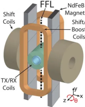
[image:15.595.226.388.291.496.2]

In figure 11 we see the schematic setup of the necessary coils in a FFL MPI scan. Two opposing NdFeB permanent magnets produce a gradient field that has a field free line along the y-axis. As the FFL needs to scan the entire xz-plane, there are shift coils in both the xand z directions. Typical TX/RX coils are used to excite the SPIONs at 20kHz in the z-direction, and receive the change in magnetization. A 3-D phantom can be placed inside the imaging bore, and is mechanically rotated about the z-axis with angle θ to create projections at different angles. Afterwards, reconstruction techniques similar to those in r¨ontgen CT enables one to reconstruct the distribution of the SPIONs across the 3-D volume.

Figure 11: Schematic setup of a FFL MPI scanner. The TX/RX coils are used as receive coils.

As we saw in section 3.3.2, it is crucial for the x-space MPI reconstruction technique to relate the received MPI signal s(t) to what is physically happening inside the imaging bore. A first step is to mathematically deduce the position of the FFL, dependent on the magnetic fields induced by all the involved coils. Fortunately, a FFL gradient for projection MPI along they direction can be constructed while obeying Maxwell’s equations. The NdFeB coils are chosen to produce the following field:

Gx=

 

G 0 0

0 0 0

0 0 −G

 

 

x y z

 

The total magnetic field inside the imaging bore is

H(x, t)=Gx+

 

Hx(t)

0

Hz(t)



. (20)

(16)

be written as   x0 y0 z0  =  

cosθ −sinθ 0 sinθ cosθ 0

0 0 1

  | {z }

R   x y z  .

Conveniently,Ris a unitary matrix soR−1=RT. Looking at (20), we can now write the total magnetic field experienced by a rotated sample in thex0 coordinate system as

H(x0, θ, t)=RGRTx’+Hx(t)ˆi+Hz(t)ˆk

(21)

To determine where the FFL lies in thex’coordinate system, it is easiest to set|H(x’, θ, t)|2_{= 0. This yields} that the field is zero at

z0 =−Hz(t) Gzz

(22)

on the line

x0cosθ+y0sinθ= Hx(t)

Gxx

. (23)

See [31] for more details. Hence, Hx(t) and Hz(t) able us to place the FFL anywhere in the xz-plane at an

orientation that we influence by the choice of θ. Similar to section 3.3.2, we will now mathematically write down the physical origin of the FFL MPI signal, as done in [31].

In section 3.3.2 we saw that in FFP MPI, the blurred 3-D MPI image originates from the dynamics given in equation (14). Forθ= 0, the change of magnetization in the field free line is projected onto thexz-plane, at the position of the FFL. Define

ρ2(x, z) =

Z

ρ(x, y, z) dy, (24)

and recall that the position xs(t) of the FFL is also totally defined through itsxz-coordinates. Therefore, the

projectionρ2(x) satisfies

˜

ρ2(x)∝ρ2(x)∗ ∗xˆ˙·h(x)xˆ˙

_x₌_x

s(t)

, (25)

where h(x)is defined as (12), withG=G2,

G2=

Gxx 0

0 Gzz

.

We identify (25) as the 2-D convolution of the PSF with the ideal projection of the nanoparticle density.

Reconstruction of FFL MPI data

For the results in this thesis, we will only consider 2-D images. For this purpose, we don’t have to consider thez-axis and simulate 1D projections of a 2-D density functionρ(x, y). If we takeN projections at anglesθi,

i∈ {1,2, .., N}, then according to the 1-D variant of equations 24 and 25, these projectionsPi are proportional

to

P(l, i) =

Z

ρ(x, y)δ(xcosθi+ysinθi−l dy

∗h(l), (26)

i.e. a projection at angle θi convolved with a point-spread function h(·). This 1-D point-spread function can

be found by using

G=

 

G 0 0

0 0 0

0 0 −G



. (27)

in equation (12), atz= 0. We do this explicitly in the next section. Now, P forms the data set after a field free line MPI scan. Such a data set is called a sinogram, and if it is rich enough (i.e. if N is big enough), it can be used to reconstruct the original nanoparticle densityρ(x, y) through a technique called filtered backprojection. As the name already reveals, it consists of a backprojection step and a filtering step. In a continuous setting, that is if we had projected along infinitely many angles θ, we could define the projections P as a continuous 2-D function P(l, θ) and the backprojection step computes

ˆ

ρ(x, y) =

Z 2π

0

(17)

In words, the equation above sums the contribution of every line that went through (x, y) when the projections where formed. In practice, the integral in this equation is a sum, as we only have a finite amount of angles

θi. After the backprojection step, a filtering step is done, because the projection of a value ρ(x0) with high

density is more often backprojected onto the points in the vicinity of x0 than points far away. This effect can be negated by a simple linear ramp filter in Fourier space.

3.5 Parallel MPI

Now that we know how MPI works and what types of reconstruction techniques are currently available, we can see if we can design an MPI system that fulfills all the requirements given in section 3.1.1. Let us go by them one by one.

1. It is possible to measure the signal at different locations. As in MRI, the source of the received signal lies within the body. The source is a change in magnetization of the SPIONs and can be picked up by a coil at any location around the body. Hence, this requirement is fulfilled.

2. There is room for undersampling while still scanning each location of the object. field free point MPI fails with this respect. As each point in the body has to be addressed to extract the nanoparticle density at that location, undersampling would simply mean that we will never know the nanoparticle density at the spots we did not visit with the field free point.

3. Except for sensitivity differences, each receive channel has to receive the same signal. Again, this fails for field free point MPI, as the coils that are placed in the excitation direction yield an image that contains fundamentally different information than coils that are perpendicular to the excitation direction..

So, requirements 2 and 3 fail for traditional field free point MPI. We now give the two key insights that enable us to do parallel MPI, using a field free line.

Key insight 1

The main reason that requirement 2 is fulfilled in MRI, is that data acquisition in MRI occurs in Fourier-space (k-space). In k-space, undersampling yields only aliasing, as opposed to the deletion of essential information that would occur in the x-space undersampling for field free point MPI. In parallel MRI, the aliasing is then unraveled using the extra spatial information of each parallel coil. Interestingly, if we look at Field Free Line MPI, the Fourier Slice Theorem tells us that FFL MPI also samples in k-space:

Theorem 3.1 (Fourier slice theorem). LetF1 andF2 be the 1-D and 2-D Fourier transform operators

respec-tively, andP1be the projection operator, that projects a 2-D function onto a line, i.e. sums the values along one

dimension. Finally, letS1 be an operator that makes a slice through the origin of a 2-D function, perpendicular

to the projection lines. Then,

S1F2=F1P1

Hence, undersampling in FFL MPI can be done without necessarily deleting deleting essential information. In this context, undersampling means taking less projection angles. From that, one could also make a second argument why FFL MPI fulfills to requirement 2: although taking less projection angles, we do still visit each part of the body, be it less often.

Key insight 2

Next, we make the most fundamental insight that proves parallel MPI is realizable. Here, knowledge of MPI physics was indispensable. The goal is to prove that, opposed to field free point MPI, in field free line MPI we can record the same change in magnetization of the SPIONs with coils placed at different locations. To do so, we have to dig into the physics, and make use of sections 3.3.2 and 3.4 .

In FFL MPI, the gradient field is

Gx=

 

G 0 0

0 0 0

0 0 −G

    x y z 

, (29)

which implies that the field free line will be along the y-axis as in figure 11. Now, as we saw in section 3.3.2, the point spread function in 3D x-space MPI is a 3x3 matrix-valued function that turns into a scalar-valued function as soon as one picks a “listening” vector and an excitation vector. Recall from equation (14), that for the gradient field given in (29), the matrix PSF will be

h(x)=ET(x)·

G x2₊_z2

 

x2 ₀ _xz

0 0 0

−xz 0 −z2



+EN(x)

   

G 0 0

0 0 0

0 0 −G

 −

G x2₊_z2

 

x2 ₀ _xz

0 0 0

−xz 0 −z2

 

(18)

whereET(x) = ˙L(||Gx||/Hsat), andEN(x) =L(_||||_GxGx_||||_/H/Hsat)

sat are the tangential and normal envelopes of the PSF.

Let us now choose the excitation and receive coil vectors. As an excitation direction, we pick the x-direction, i.e. [1 0 0]. We place the multiple receive coils in the xy-plane atz = 0, so that their positions are given by [cos(θ),sin(θ),0]. The resulting PSF is then

h(x, z) = [cos(θ),sin(θ),0]·h(x)·

 

1 0 0



=Gcos(θ)

ET(x, z)

x2

x2₊_z2+EN(x, z)

1− x

2

x2₊_z2

(31)

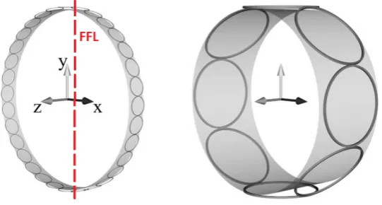
[image:18.595.168.439.273.418.2]

Hence, the images received by the different coils in the xy-plane are only different by a factor! This is proves that FFL MPI with this coil setup fulfills requirement 3. Another nice observation here, is that if we place the center of the receive coils atz= 0, the normal envelope of the point spread function is multiplied by zero. Hence, FFL MPI gives a better resolution in thexy-plane, than FFP MPI. In thez-direction the normal envelope does play a role, of course. In figure 12, two examples of receive coil setups for parallel MPI are given. The amount of receive coils has to be chosen carefully, influenced by practical hardware issues, sensitivity simulations and computational complexity. We talk more about this in section 7.

Figure 12: Two illustrative receive coil setups, with FFL orientation. The excitation of the FFL will be in the

x-direction.

Hardware setup

We will run simulations and show results for one hardware setup, that we deem best for now. In future re-search, the reconstruction qualities of several setups can be investigated and optimized, which can be a whole new project on its own.

(19)

[image:19.595.211.385.66.273.2]

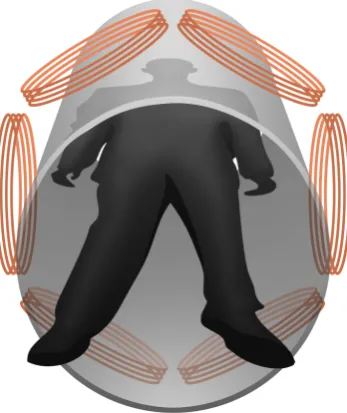
Figure 13: The receive coil setup we will consider in this project. Thez-axis is along the bore, and the centers of the six receive coils are placed at z=0. Thex-axis runs from left to right in this image, and the field free line will be parallel to they-axis, exciting in thex-direction. In this way, an axial slice of the body can be imaged with high resolution in the xy-plane.

This hardware setup implies that we have six sensitivity maps Si, shown in figure 14. To calculate these

sensitivity maps, we used a numerical Biot-Savart law simulator.

[image:19.595.108.490.382.577.2]

(20)

3.6 The parallel FFL MPI physics simulator

Currently, there is no MPI scanner in the world with a parallel coil hardware setup. Hence, in the time scope of this thesis, it is impossible to work with real data. To generate synthetic data, the easiest would be to use our operator E, that we will define later in equation (36). This can be a good first step, but will always yield better results than one can expect in real life. This is because the algorithm tries to find the best ˆρsuch that

Eρˆ=d, and if dwas created using Eρwe can even expect to find back the exact solution ˆρ=ρ. In real life however, the operatorEis just an approximation of what physicaly happens, so thatEρwill always differ from the actual data, even if there would be no noise involved.

[image:20.595.95.498.336.474.2]

Therefore, to really validate our model and reconstruction techniques, we have built a parallel FFL MPI simulator in Python. It takes the true nanoparticle density ρas an input, after which it places the field free line over the first column of the matrix ρ, and records the change in magnetization when the field free line is moved to the next column. This mimics excitation in the x-direction, which is part of our chosen strategy from section 3. The recorded change in magnetization over the entire volume is then gridded onto the correct box in the sinogram. All the paramaters, like gradient field strength and nanoparticle diameter are chosen at fixed, common values. Varying these would not yield relevant information for this project. After forming the sinogram, we can use either filtered backprojection or parallel imaging to find ˆρ. For the reader’s illustration, we show the output of the simulator whenρis the Cal phantom (logo of the University of California in Berkeley), and its reconstruction in figure 18. Note that the output in (c) is blurred, inherently by MPI physics. We do see that resolution is still pretty good, which reflects the fact that FFL MPI gets rid of the ‘bad’ normal envelope of the point spread function in thexy-plane, like we showed in the previous section.

Figure 15: The sinogram (b) is formed after the cal phantom (a) has been fed to the FFL MPI simulator, using 180 projection angles. (c) is the filtered backprojection reconstruction. Note that it is blurred by the MPI physics.

4 Inverse problem formulation.

In section 3, we saw that parallel MPI is physically feasible. The next step, is to exploit the extra spatial information that we get from the multiple coils. We can learn from the two examples in section 3.1 that it makes sense to take a forward model approach. After all, by theorem 2.1 the Fourier transforms of the MPI projections can be understood as radially sampled spokes through the origin of the 2-D Fourier transform of the nanoparticle density. Undersampling in the number of spokes will yield untraceable aliasing, which is why a direct reconstruction approach will fail.

4.1 Notation and basics

In mathematics, an imageuis treated as a function that maps values onto a domain Ω:

u: Ω→_R.

Now, whenever one wishes to visualize these functions, the domain Ω will have to be discretized, anduwill be a matrix. For Ω∈RN_{, we define}

Ui1,...,iN =

R

pixel(i1,...,iN)u(x) dx

R

pixel(i1,...,iN)1 dx

(21)

In every imaging modality, the received data of a scan - may it be a click on the button of your camera or an MRI scan - is used to form an image. How the transition from the received data to the eventual image takes place, is determined by the physical properties of the imaging system that makes the scan. In most modalities, this transition from signal to image can be described by an operator, i.e.

Eu=d (33)

where dis the received data,uis the desired image and E is the operator that describes the relation between the signal and the image. Equation (33) is called the forward model the imaging system. An intuitive approach to solveufrom (33) is to multiply both sides by theE−1_{, i.e. the inverse operator. But here two main problems} arise:

1. The inverse operator is not defined.

2. The received data d might not be equal to the theoretically expected data, due to for example noise differences caused by properties of the hardware in the imaging system. It is a hard task to nicely extract

ufrom such a signal.

Problem 1 occurs in this thesis, and a good example of problem 2 occurs when one tries to reconstruct u when

E is a convolution operator, i.e.

d=Eu=h∗u. (34)

Wherehis the so called point spread function (PSF). From the convolution theorem we know that

F(d) =F(h∗u) =F(h)· F(u).

And thus

u=F−1

F(d)

F(h)

. (35)

(22)

4.2 Forward model formulation for parallel MPI

In field free line MPI, the desired image is a blurred 2-D nanoparticle density distribution ρ, that we aim to reconstruct from projection datad. We have to be careful in the definition of our forward operatorE, because it is not our goal to deconvolve the blurred density with the point spread function. Hence, we will only put projection operations into E, and no convolutions. So from now on we will aim to reconstruct ˜ρ, being the Langevin-blurred version of the true nanoparticle density distributionρ.

Now, let L be the number of coils used in the data acquisition. The data set d after a parallel field free line MPI scan, will consist ofLsinogramsPi,i∈ {1,2, ..., L}. LetSi be the sensitivity map of coili, andRbe

theradon transform, that performs the discrete version of equation (26). We can then write

Eρ˜= [RS1ρ, RS˜ 2ρ, ..., RS˜ Lρ˜]T =d, (36)

so we will regard our data set das a multidimensional array of sizeN×M×L. N is the number of projection angles andM is usually chosen to be aboutn√2 if we aim to reconstruct a ˜ρof sizen×n. This choice follows from the Pythagorean theorem, as we have to be able to project along the diagonal of the square image.

4.3 Image reconstruction via minimization

In section 4.1 we saw that in general, problems arise in extracting the desired image from a data set. To work around this, we can rewrite the forward model to a minimization problem, and use algorithms that aim to get as close to the true solution as possible. Ideally, we can also include prior knowledge of the solution in this minimization problem. The objective function is made convex such that a minimum is guaranteed, and as a first step we consider:

ˆ

u= min

u∈X F(u) :=||Eu−d||

2

2 (37)

Setting d_dF_u = 0 yieldsEu=d, which proofs that the argmin ofF is the desired image. Also,||Eu−d||2 2, is the squared L2 _{norm of the distance between} _Eu _and _d_{, makes sure that} _Eu _{is close to} _d_{. Conformly, this term} is called the data fidelity term. Now, as in section 4.1, significant noise will cause problems if we try to find the minimum ofF through an algorithm. Therefore, we can choose to extendF with a second term called a regularization term, that guides the algorithm in the right direction. We will talk more about this in section 5. Besides the forward operator, the algorithm needs another operator to find the minimum of the objective function: the adjoint operator E∗. Let E :X →Y, then the adjoint operator is defined as the operator that satisfies the equation

hEp, qiY =hp, E∗qiX, (38)

for all possible p∈X andq∈Y. Hereh·,·iX andh·,·iY are the innerproducts on X andY respectively. The

adjoint operator is in practice more often defined and easier to find than the inverse operatorE−1. The reason that a minimization algorithm needs this operator, can be seen if we would analytically try to solve equation (37).

dF

du =E

∗₍_Eu₋_d_{) = 0} ₍₃₉₎

(E∗E)ρ=E∗d (40)

We see two things here. Firstly that the adjoint operator plays a role in calculating the derivative of the objective function as we see in (39). Secondly, we see that if we can findE?, we can solve (40) instead of (37). This can be convenient, because there are very efficient algorithms, e.g. the conjugate gradient algorithm, that exploit the fact that (E∗E) is self-adjoint and positive definite. Therefore, we need to find the adjoint operator

(23)

4.4 The adjoint operator for parallel MPI

To find the adjoint to the forward operator defined in equation (36), we can use the definition of the adjoint operator. The first observation we make, is that for the inner product in (38) to be defined, we needE?_:_Y _→_X_,

with ρ∈X and d∈Y. Furthermore, we use the following: letA, B :X →Y be two operators. Then for all

x∈X andy∈Y, by definition of the adjoint operator we have

hABx, yi=hBx, A∗_yi₌_{hx, B}∗_A∗_yi.

So (AB)∗ =B∗A∗. Hence, with E given in (36), for eachRSi we use (RSi)∗ =Si∗R∗ to find E∗. IfLreceive

coils are used, we obtain

E∗d= [S₁∗R∗, S₂∗R∗, ..., S_L∗R∗]

    

d1

d2 .. .

dL

    

(41)

=

L

X

i=1

S_i∗R∗di, (42)

where S_i∗=Si as it only performs a pointwise, real matrix multiplication. Furthermore, it is well known that

backprojection is the adjoint operator of the radontransformR. So, forR∗we use equation (26). The backpro-jection operation transforms each di into ann×n matrix, yielding Lmatrices. The pointwise multiplication

(24)

5 Convex optimization and regularizers

5.1 Convex functions

As discussed in section 4.3, the reconstruction problem for parallel MPI can be written as a minimization problem. Whenever an analytical solution to such a minimization problem is unavailable, numerical techniques have to be used. To guarantee the existence of a solution, it is essential that the objective function is convex. Let us start this section with the very definition of a convex function.

A functionF :X →Ris called convex if for allx1, x2∈X andλ∈[0,1]

F(λx1+ (1−λ)x2)≤λJ(x1) + (1−λ)J(x2).

F is strictly convex if the inequality is strict. Convex functions have the nice property that every one of its minima is a global minimum, and if they are strictly convex, the minimum is unique. In imaging, the functions involved in (43) are often convex, as they are chosen to be the norm of a Banach space. In this chapter, we will first extend the objective function to our needs, and do a quick review on the theory of convex minimization that is most relevant for this project. With that knowledge, we will regard algorithms that can compute the minimum of the convex objective function.

5.2 Regularization

In addition to the data fidelity term in (37), a regularization term can be included in the objective function to penalize certain unwanted properties of the solution ˆu, and to improve the condition of the minimization problem. Most of the time, these two go hand-in-hand. In the objective function, one places a factor λ to adjust the severity of the regularization.

ˆ

u= min

u∈X E(u) := λH(u)

| {z }

Data fidelity

+ J(Au)

| {z }

Regularization

. (43)

Before minimizing (43), a specific regularization term J has to be chosen. This is quite an important choice, because it imposes restrictions and properties on the solution ˆu. We will define the most important spaces in which these solutions can live and their (dis)advantages in section 5.2.1. We now make a head start by regarding two examples that entail the two most famous spaces on continuous domains, so that the reader gets a feeling for what formulation (43) can do.

The data fidelity term we will regard is

H(u) = λ

2||Eu−d|| 2 2,

which is a distance measure between Eu andd and minimizing this is the most fundamental requirement; if we leaveH(u) out of the objective function, we end up with a solution that has no connection to the datadat all. Note that we need u∈L2_{(Ω) in order for}_H₍_u_{) to be finite. Fortunately,}_L2_{(Ω) is a very rich space, and} we thus have a big pool of images to obtain a solution from. For the regularization term, a first choice would be J(u) = 0. To give an illustration of how this works in the framework of (43), we regard our convolution problem in (34). We have

ˆ

u= min

u∈L2_(Ω)

1

2||h∗u−f|| 2

2. (44)

Taking the derivative w.r.t. utogether with Plancherel’s theorem and the convolution theorem yields that we end up with the same solution ˆuand thus problems as in (35). Hence, we must use a nonzero regularization term. Let us setJ(u) = 1

2||u|| 2

2; as this is finite for allu∈L2, we preserve the large amount of images that we can extract a solution from. So, we have an explicit minimization problem:

ˆ

u= min

u∈L2_(Ω) ·

λ

2||h∗u−f|| 2 2

| {z }

Data fidelity

+ 1₂||u||2 2

| {z }

Regularization

. (45)

Which, by convexity, has a unique solution, and it is

hatu=F−1 F(h)F(f)

|F(h)|2₊ 1

λ

!

. (46)

(25)

L2_{(Ω), which makes it unsuited for denoising purposes.}

Hence, we look for a space in which we have an improved condition of the problem as in (46), but at the same time improve the signal to noise ratio (SNR) of ˆu. Noise is characterized by fast movements in the signal intensity, i.e. high derivatives. Therefore, we introduce J(u) = 1₂||∇u||2

2 to penalize derivatives, and end up with the minimization problem

ˆ

u= min

u∈H1_(Ω) ·

λ

2||Ku−f|| 2 2

| {z }

Data fidelity

+ 1₂||∇u||22

| {z }

Regularization

. (47)

Using directional derivatives and Plancherel’s theorem, one can deduce that there is a unique solution to this minimization problem:

F(ˆu)(ω) = F(h)(ω)F(f)(ω)

|F(h)(ω)|2₊1

λ|ω|2

. (48)

The inverse Fourier transform gives then the best approximation ˆuto the true image. We see that division by zero is avoided and the high frequency parts are explicitly damped, so noise is reduced instead of amplified.

[image:25.595.74.536.340.611.2]

In figure 16 , we show the results of L2 and H1 regularization on a 1-D image that is subject to a convolution with a Gaussian kernel, and white noise. We omit the plot here, but we want to stress that without regulariza-tion, the deconvolution yields a completely blown-up signal that contains no information about the true image.

(26)

5.2.1 Spaces of images

The two examples in the previous section have shown us that regularization can help to prevent noise blow-ups in reconstruction techniques, but that caution is needed. Namely, we saw that the choice of the regularization term affects the space X in which we look for a solution. Firstly because we need the regularization term to be finite. Secondly, when we derive the optimality condition for the solution of the minimization problem, we can derive certain properties of the solution. More on this follows in section 5.2.2.

The relation between this requirement and the space X is found in the very definitions of these spaces. We start with the Lebesgue spacesLp_{. For every 1}_≤_{p <}_{∞ ∈}

Rwe have

Lp(Ω) :=

u: Ω→_R :

Z

Ω

|u|p_d_{x <}_∞

(49)

Note that Ω can be any subset ofRn. Another important space is

L∞(Ω) :=

u: Ω→R : ess sup

x∈Ω

u(x)<∞

(50)

because we can denote a function’s maximum through the L∞ norm. Every Lebesgue space with p≥1 is a Banach space with norm

||u||Lp=

Z

Ω

|u|p _d_x

1_p

||u||L∞ = ess sup

x∈Ω

u(x)

Forp= 2,Lp _{is a Hilbert space, defined by the inner product}

hu, viL2 :=

Z

Ω

u·v dx (51)

A motivation for choosing a Lebesgue spaces as an image space, is that they are very big. For example, images with a countable number of discontinuities are allowed, which is great because every edge in an image is characterized by discontinuities. Moreover, we know that forp >1, each Lebesgue space is a dual space, since

Lp(Ω) = (Lq(Ω))∗⇐⇒ 1

p+

1

q = 1. (52)

As we shall see in section 5.3, dual spaces are especially nice in the sense of minimization problems for convex functionals.

Yet, Lebesgue spaces have their drawbacks. This is mainly due to the fact that they are not able to clearly distinguish between noise and signal. That is, the Lp norm of a signal with added Gaussian noise is not nec-essarily larger than that of the original signal. Therefore, we look for normed subspaces of Lp that are in fact able to detect noise through their norm. An obvious consideration is to look at the Sobolev spaces that involve the first-order (weak) derivatives:

W1,p(Ω) =

u∈Lp(Ω) :

Z

Ω

|∇u|p dx <∞

. (53)

So we see immediately that W1,2_(Ω) _⊂ _L2_{(Ω). The restriction is caused by a property that we like for our} imaging purposes: the weak derivative∇uhas to bep-integrable. This makes us able to distinguish noise from signal because the Sobolev seminorm

|u|p_W1,p=

Z

Ω

|∇u(x)|p _d_x ₍₅₄₎

of an image that is subject to noise is relatively large. Therefore, it is smart to use this Sobolev seminorm as the regularization term J, to create a penalty on noisy images. We will now dig a little deeper into the effects that these choices for J have on the properties of the solution of (43), see if disadvantages arise and how we can adapt to them.

5.2.2 Properties of the solution to the objective function.

(27)

precise description of the properties of ˆu. Subsequently, we suggest a regularization term that does a better job at keeping sharp edges in place.

To give an illustration, let us start with the most simple case

ˆ

u= min

u∈L2_(Ω) E(u) =_u_∈min_L2_(Ω) λ

2||Ku−f|| 2

2+12||u|| 2 2.

Where K is an integral operator, such as the convolution in (34). The optimality condition then yields

0 =E0(u) =λK∗(Ku−f) +u

=⇒ u=λK∗(f −Ku)

Souis in the range ofK∗, which is again an integral operator. This implies that ˆuwill be smooth and contains no sharp edges. So even forL2 _{regularization on a signal that contains very little noise, we might not end up} with the solution we want.

Next, for noisy signals we wish to use a penalty on the derivatives:

ˆ

u= min

u∈H1_(Ω) E(u) =_u_∈min_H1_(Ω) λ

2||Ku−f|| 2 2+ 1 2||∇u|| 2 2. The optimality condition yields

0 =E0(u) =λA∗(Ku−f) +∇∗_∇u ₍₅₅₎

=⇒ u=λ(∇∗∇)−1K∗(f−Ku) (56)

For simplicity consider K=I, and recall that ∇∗=−div and thus ∇∗∇=−∆. Hence, (56) simplifies to ∆u=λ(f−u), f−u∈L2(Ω)

which is an elliptic partial differential equation (PDE). From elliptic regularity [26], we know that the solution to this PDE will live inW2,2_{(Ω) and thus be oversmoothed. This analysis gives rise to a key question: can we} design a regularization functional J(u) that penalizes derivatives and at the same time allows for solutions ˆu

to (43) that contain sharp edges?

To answer this question, we look at the properties of a more general regularization term

J(u) = 1

p

Z

Ω

|∇u|p_d_x. ₍₅₇₎

Then, the optimality condition yields

0 =E0(u) =λK∗(Ku−f)− ∇· _|∇u|p−2_∇u

. (58)

The Euclidean norm of |∇u|p−2_∇u_is _|∇u|p−1_{. So when} _{p >} _1,_∇u _{will have such a big impact on the value} of ∇∗ _|∇u|p−2_∇u

for images uthat contain large “gradients”, that the data fitting is too heavily distorted. Remember that very large gradients are present at the edges of images. Therefore, for p >1 the solution to (58) will not contain any sharp edges even though the data fidelity term tells us so. Interestingly, we see a shift in this behavior whenp↓1. The Euclidean norm of|∇u|−1_∇u_{is equal to 1, no matter how large} _∇u_{. Hence,} forp= 1, images with large (infinite) “gradients” can still be a solution to (58). We have to be careful, though. The reason we write “gradients”, is that for functions that contain discontinuities, the gradient is not defined. Therefore, we introduce the concept of total variation.

5.2.3 Total variation

The total variation (TV) of a function is defined as

T V(u) :=

Z

Ω

|∇u|dx, (59)

which makes sense only if u ∈ W1,1_{(Ω). Now, piecewise constant functions that contain discontinuities, are} not inW1,1_{(Ω). Therefore, we consider a larger space: the space of functions of bounded variation}_BV_{(Ω). To} define this space, we must first give the exact definition of the total variation:

T V(u) := sup

g∈C₀∞(Ω;Rd)

||g||∞≤1

Z

Ω

(28)

For now we use

||g||∞:= ess sup

x∈Ω

p

g1(x)2₊_...₊_g

d(x)2,

but variants of this choice are possible as well, leading to different properties of solutions. The space of functions of bounded variation is then defined as

BV(Ω) :=

u∈L1(Ω) :T V(u)<∞ (61)

i.e. the space of functions for which the total variation is well-defined. A short summary: We saw that for

p↓1, the solutions to the convex minimization problem

min

u λ

2||Eu−d|| 2 2+

1 2

Z

Ω 1

p|∇u| p _d_x

are not oversmoothed. Hence we like to usep= 1, but the gradient operator∇is only defined foru∈W1,1_(Ω), which does not allow for sharp edges. Therefore, we defined the concept of total variation, sinceT V(u) is finite for piecewise constant functions u, and is equal to ∇ufor u∈W1,1_{(Ω). So, we look for the minimum of the} convex functional

min

u∈BV(Ω)

λ

2||Eu−d|| 2

2+T V(u) (62)

(29)

5.3 From theory to practice

In this project, we are going to consider the following objective functions:

min

u λ||Eu−d||

2

2+||Au|| 2

2 , A= 0, I or∇, (63)

min

u λ||Eu−d||

2

2+||∇u||1 (64)

For (63), the optimality condition yields that it is equivalent with solving

(λE∗E+A∗A)u=λE∗d,

which we will do using the conjugate gradient algorithm that we introduce in section 5.4.1 as the operator (λE∗E+A∗A) is self-adjoint. For the objective function in (64) with the L1 norm present, we have to put in some more effort. The optimality condition yields

(λE∗E)u− ∇ ·

∇u |∇u|

=E∗d,

which brings about two problems. Firstly, we identify a possible division by zero. Secondly, if one would somehow circumvent this division by zero (for example by adding a small number ), we are again left with a PDE that has smooth solutions, while we wish to preserve discontinuities (edges). There are two ways to proceed. One is to approximate J = |∇u| by ˆJ = p(∇u)2₊_{, because it tends to favor diffusion along} edges rather than accross, so that edges are smoothed out less than other structures [41]. Most of the time, it performs sufficiently well but it is a trick and an approximation. We take the second, more general and accurate approach. It makes use of theFenchel duality theorem. This states that to every primal problem

P = min

u∈X H(u) +J(Au), (65)

there exists a dual problem

D= max

p∈Y∗ −H

∗₍_A∗_p₎₋_J∗₍_−p₎ ₍₆₆₎

such that E =B. Note thatH : X →[0,∞] andJ :Y →[0,∞] are assumed to be convex functions. The functions H∗ _and_J∗ _{that are found in the dual problem, are called the} _{convex conjugates} _of _H _and_J_{. They}

can be found explicitly , and are defined as follows. Let F be a convex function of a vector z∈ Z, then the convex conjugate is defined as the Legendre transform ofF:

F∗(˜z) = max

z {hz,zi −˜ F(z)}. (67)

The original function F can be recovered by applying conjugation again:

F(z) = max ˜

z {hz, zi −˜ F

∗_(˜_z₎_}_. ₍₆₈₎

Now, to see why this helps us solve (64), we will circumvent the problems with the minimization of theL1_term by substituting it with its convex conjugate, to create a saddle point problem. By definition,

J(Au) = max

p {hAu, pi −J

∗₍_p₎_}_,

so we can rewrite (65) into the saddle point problem

S := min

u∈X pmax∈Y∗ hAu, pi+H(u)−J

∗₍_p₎_. ₍₆₉₎

In section 5.4.2, we introduce a primal dual method that solves (69). It uses an optimality condition based on the concept of subdifferentials, and the difficultL1minimization we had in the primal problem transforms into a simple projection onto a convex set in the dual space, characterized by one update rule in the algorithm.

Subdifferentials and the optimality condition

(30)

Let F : X → R be a convex functional and X∗ be the dual space of X. Then, the subdifferential of F at u∈X is defined as

∂F(u) ={p∈X∗ : hp, v−ui ≤F(v)−F(u), ∀v∈X} (70) whereh·,·idenotes the standard duality product betweenX andX∗. An elementp∈∂F is called a subgradient and can be identified with the slope of a plane in X ×R through (u, F(u)) that lies under the graph of F.

From the definition we can see immediately that û is a minimizer of F if and only if 0 ∈ ∂F(û), and due to convexity this first-order optimality condition is not only necessary but also sufficient. Another important notion on subdifferentials is that for Fréchet-differentiable functionals, the subdifferential coincides with the classical derivativeF0(u).

5.4 Algorithms

Up to now, we have formulated the inverse problem for parallel MPI and all its components. Also, we showed that it can be rewritten as the minimization of a convex objective function, to which we can add convex regularizers to improve the condition of the problem, especially when the data is noisy. We selected two algorithms that can solve these minimization problems: the Conjugate Gradient (CG) algorithm, and a primal dual hybrid gradient (PDHG) method. The CG algorithm is very efficient, but problems arise when we add the TV regularizer to the objective function. The PDHG algorithm is perfectly suited for the latter, and very flexible.

5.4.1 Conjugate gradients

This efficient algorithm solves any problem

Ku=d

as long asKis a self-ajoint and positive definite operator, and it is so efficient because it exploits both of these properties. As discussed in section 5.3, we can write the objective functions in (63) such that a specific operator

K is formed that is positive definite and self adjoint. we feed the operator K and the data dto the following iteration scheme:

Algorithm 1 Conjugate gradient algorithm

Chooseu0_∈_X_{, let}_r0₌_d₋_Ku0 _and_p0₌_r0_.

forn =0,1,2,...do

                          

αn= ₍_p(rnn₎⊥)⊥_Kprnn un+1₌_un₊_αn_pn

rn+1=rn−αnKpn βn =(r₍n_r+1n₎⊥)⊥_Krrnn+1 pn+1₌_rn+1₊_βn_pn

end for

5.4.2 Primal-dual hybrid gradients

To solve the saddle point problem (69), we use a so called first-order primal-dual hybrid gradient method, in-troduced by Chambolle and Pock [27]. This algorithm is great in its simplicity, and still has a good convergence rate.

Assume that there is a solution (ˆu,pˆ) to (69), then we know that we must have

0∈∂S(ˆu) (71)

0∈∂S(ˆp). (72)

Now, as the inner producthAu, piis Fr´echet differentiable, we can use the classical derivative for this term in

S, and see that (71) and (72) are equivalent with

Auˆ∈∂J∗(ˆp), (73)