Testing the expectations theory of the term structure of interest rates in threshold models

University of Warwick institutional repository: http://go.warwick.ac.uk/wrap

This paper is made available online in accordance with

publisher policies. Please scroll down to view the document

itself. Please refer to the repository record for this item and our

policy information available from the repository home page for

further information.

To see the final version of this paper please visit the publisher’s website.

Access to the published version may require a subscription.

Author(s): MICHAEL P. CLEMENTS and ANA BEATRIZ C. GALVÃO

Article Title: TESTING THE EXPECTATIONS THEORY OF THE TERM

STRUCTURE OF INTEREST RATES IN THRESHOLD MODELS

Year of publication: 2003

Link to published

TESTING THE EXPECTATIONS

THEORY OF THE TERM STRUCTURE

OF INTEREST RATES IN THRESHOLD

MODELS

M

P. C

A

B

C. G

˜

We test the expectations theory of the term structure of U.S. interest rates in nonlinear systems. These models allow the response of the change in short rates to past values of the spread to depend upon the level of the spread. The nonlinear system is tested against a linear system, and the results of testing the expectations theory in both models are contrasted. We find that the results of tests of the implications of the expectations theory depend on the size and sign of the spread. The long maturity spread predicts future changes of the short rate only when it is high.

Keywords:Term Structure, Expectations Theory, Threshold Models

1. INTRODUCTION

A number of recent studies of the term structure of U.S. interest rates look for possible asymmetries in the response of the short-term interest rate to spreads between long and short rates; earlier work has tested the expectations theory of the term structure by imposing restrictions in vector autoregressive (VAR) models, following Campbell and Shiller (1987), or by regressions of the change in short rates on the lagged spread [see, e.g., Mankiw and Miron (1986)]. The work on asymmetries in the response of the short-term interest rate has generally been based on equation threshold models for the short rate. We show that single-equation nonlinear threshold model testing and specification techniques can be adapted to permit joint modeling of the short-term interest rate and the spread, and that some of the tests proposed by Campbell and Shiller (1987) can be applied in such a framework. The systems approach yields interesting insights into the

We acknowledge the helpful comments of two anonymous referees. Financial support from the UK Economic and Social Research Council under grant L138251009 is gratefully acknowledged by the first author, and from Capes-Brazil by the second author. The computations reported in this paper were performed using code written in the Gauss Programming Language. Address correspondence to: Michael P. Clements, Department of Economics, University of Warwick, Coventry CV4 7AL UK; e-mail: [email protected].

c

dynamic behavior of the variables, and we are able to interpret the estimated models in terms of recent work on the term structure of interest rates.

Sola and Driffill (1994) are perhaps closest to our approach, in that expecta-tions theory restricexpecta-tions are applied in a bivariate VAR of 3- and 6-month interest rates in which the means and equation error variances are permitted to follow an unobserved Markov process. Matching Hamilton (1988), they find that the 1979–1982 period, when the Federal Reserve changed its operating procedures, is associated with a different regime than the periods 1962–1978 and 1983–1990. Furthermore, the expectations theory restrictions are not rejected in the Markov-switching model, although they are in a constant-parameter, linear VAR. In addition to 3- and 6-month rates, we consider 3-month and 10-year interest rates, extend the sample to include the 1990’s, and allow up to three regimes, with the regime in force at any period being determined by the (lagged) value of the spread, rather than being exogenously given, as in the Markov-switching approach.

The dependence of the regime on the spread is a potentially attractive feature because it explicitly models the idea that adjustment to equilibrium in financial markets may depend on the sign of the disequilibria and may not vary propor-tionately with its size. In that case, linear equilibrium-correction models will be inappropriate. The frequently cited example is of transactions costs, whereby ar-bitrage opportunities between two markets only arise when the price differential is large enough to imply net gains to traders. As a consequence, nonlinear equi-librium correction models have been used to model the relationship between spot and future prices by, inter alia, Dwyer et al. (1996), Martens et al. (1998), and Tsay (1998), and between interest rates of different maturities by, for example, Anderson (1997), Enders and Granger (1998), van Dijk and Franses (2000), and Hansen and Seo (2001).

The plan of the remainder of this paper is as follows: Section 2 reviews vector equilibrium-correction models (VECM’s) of the term structure, and VAR-based tests of the expectations theory. The specification and testing procedures for thresh-old VECM models are recorded in Section 3, and the empirical results are presented in Section 4. The relative forecast performance of a number of linear and nonlinear models of interest rates are considered elsewhere [Clements and Galv˜ao (2001)]. Section 5 draws out the economic implications of our results and relates these to the recent literature. Section 6 concludes.

2. TERM STRUCTURE OF INTEREST RATES AND EQUILIBRIUM CORRECTION MODELS

The simple expectations theory implies that the k-period interest rate is the weighted average of the expected future one-period interest rates plus a risk premium:

rt(k)=

1 k

_k

j=1

Etrt+j−1(1)

wherert(s)is thes-period interest rate att,Et is the expectations operator

con-ditional on timet, and Lt(k)is the term premium, which may reflect risk and

liquidity premia. Arbitrage between bond markets with different maturities will ensure that this condition holds, while the presence of the term premium will gen-erally result in the yield curve [rt(k)plotted againstk] being upward sloping. If rt(1)is integrated of order one [I(1)], then so isrt(k)from (1), and interest rate

spreads areI(0), because (1) can be written as

St(k)≡rt(k)−rt(1)=

1 k

_k−1

i₌1 i

j₌1

Etrt+j(1)

+Lt(k) (2)

= 1

k k−1

j₌1

(k−j)Etrt+j(1)+Lt(k) (3)

[see, e.g., Hall et al. (1992)]. The RHS is the sum of a finite number of I(0) terms (ignoring the risk premium) and is thereforeI(0). Thus,rt(k)andrt(1)are

cointegrated with weights [1−1], as are any two yields of different maturities. By the Granger representation theorem, cointegration implies the existence of a VECM, viz.

rt =Φ(L)rt−1+α(St−1−µ)+εt, (4)

wherert=[rt(l),rt(s)]denotes the vector of the long (k=l) and short-term rates

(s=1);Φ(L)is a matrix of coefficients in the lag operator,L, withLn_x

t=xt₋n,

and=1−L the difference operator.St is the spread andµis the equilibrium

spread; they may differ from zero because of the term premium. The adjustment vector to the long-run attractor isα.

2.1. Expectations Theory

To make matters concrete, we suppose thatΦ(L)is first order, so that we have lag 1 and lag 2 terms in the changes inrt(l)andrt(s):

rt =c+ 2

j₌1

Φjrt−j+αβrt−1+εt, (5)

whereβ=[1 : −1], so thatβrt₋1=St₋1 defines the spread. As Campbell and

Shiller (1987) note, because by equation (2) the spread is a linear combination of future changes in the short rate [plus Lt(k)], it should help predict the values

premultiplying (5) byB, where

B=

1 −1

0 1

to give

Brt =Bc+ 2

j₌1

BΦjB−1(Brt−j)+BαSt−1+Bεt, (6)

whereBrt=[Strt(s)]. Whenαis not the zero vector (so that the twoI(1)interest

rates are cointegrated with vector [1:−1]), equation (6) can be rearranged to give a VAR inr∗t =[St rt(s)], withvt=Bεt,c∗=Bc, and suitably defined coefficient

matrices11_:

r∗t =c∗+Γ1r∗t−1+Γ2r∗t−2+Γ3r∗t−3+vt. (7)

If, however,α=0, the levels term in the interest-rate spread is absent from (6), so thatSis integrated of order 1, and the VAR corresponding to (7) is in [St rt(s)],

so that there are restrictions on theΓiin (7) such thatShas a unit root [and, in

addi-tion,Γ₃=0 ]. Therefore, the VAR is constructed on the assumption that the theoret-ical implication of the expectations theory—thatr(l)andr(s)are cointegrated— holds.

Because the expectations theory posits a relationship between the spread and predictions of future changes inr(s), it will prove useful to write (7) in compan-ion form, whence the predictcompan-ions have a relatively simple analytical form. The companion form is

Rt =C+ΓRt−1+Vt, (8)

where

Rt=

r∗t

r∗t−1

,C=

c∗ 0

,Γ=

_Γ

1 Γ2 I2 0

,Vt =

vt 0

.

We defineiS=[1 0 0 0] andir=[0 1 0 0], so thatSt=iSRtandrt(s)=irRt.

At this point, we note two versions of the expectations theory. Underlying the stronger version of the theory is thatLt(k)=θin (2), so that the term premium is

constant. Then, taking expectations dated periodtof both sides of (2) gives

EtSt ≡St =

1 k

_k−1

j=1

(k− j)Etrt₊j(1)

+θ. (9)

As Sola and Driffill (1994, p. 604) note, it is common to posit a slightly weaker version that allows for a random error term in the relationship between long-and short-term rates, so that Lt(k)=θ+ut, whereθ is again the constant term

premium andutrepresents measurement error or random variation in the premium.

expectations taken at periodt−1, so that, from (2),

Et₋1St =

1 k

_k−1

j=1

(k−j)Et₋1rt₊j(1)

+θ, (10)

where we use Et₋1Et(·)=Et₋1(·). We entertain both possibilities, noting that a

key attraction of (9) is that it can be applied directly in the context of threshold models, at least fork=2, as explained in Section 2.2.

2.2. Cross-Equation Restrictions in the VAR

Beginning with (10), the LHS of this expression from (8) is isC+isΓRt₋1. To

evaluate the RHS of (10), note that

Et−1rt+j(1)=irEt−1Rt+j=ir

C

j

s=0

Γs_+Γj+1

Rt−1

.

In Appendix A, we derive the following approximate expression for the term in

Rt−1for the RHS of (10) (omittingθ), for largek:

irΓ2(I−Γ)−1Rt₋1.

By equating coefficients onSt−1on both sides of (10) and rearranging, we obtain

isΓ(I−Γ)=irΓ2. (11)

Whenk=2, equation (10) simplifies to Et−1St=1₂[Et−1rt+1(1)]+θ, so that

substituting from the VAR gives

isC+isΓRt₋1=

1 2ir

C 1

s=0

Γs+Γ2Rt₋1

+θ. (12)

Equating coefficients onRt−1again gives four cross-equation restrictions on the

coefficients in the VAR:

isΓ=

1 2irΓ

2_{. (13)}

The restrictions for k=2 and the largek case in terms of the elements of the matrices of the VAR are detailed in Appendix B.

Fork=2, the stronger version of the theory impliesisRt≡St=1₂irEt[Rt₊1]+

θ=1

2ir[C+ΓRt]+θ, so that the restrictions are (equating coefficients onRt) is=

1 2irΓ

and, for largek,

These restrictions are also detailed in Appendix B.

Fork=2 and the stronger version of the theory, we can readily calculate the “the-oretical” spread from the VAR because the one-step-ahead predictions ofrt+1(s)

are simply the fitted values in the VAR equation forrt+1(s)(we replace the

un-known parameters in the VAR with their full-sample estimates of their values). Therefore, the theoretical spread (S) is simply one-half times the fitted value. More generally, as in Campbell and Shiller (1987, p. 1080, Fig. 1), plots ofStand Stunder the expectations theory can be obtained using the VAR-based predictions

of the short rate to evaluate the RHS of (9) to giveSt.

In the case of largek, the long-term bond carries coupons, which have a higher present value in the near future than in the distant one. Therefore,Stcan be modified

accordingly to take into account weights declining monotonically with the time horizon j:

1 1−gk

k−1

j₌1

(gj−gk)irEt[Rt+j], (15)

where g is an approximation for returns on bonds selling close to par, that is, g=1/[1+µr(l)], given that µr(l) is the average of the long-term rate [see

Hardouvelis (1994)]. These weights are based on a linearized approximation to the yields on coupon bonds and(1−gk_{)/(1−g)is the “duration” of ak-period}

bond.

2.3. Granger Causality of the Short Rate by the Spread

The weaker restriction implied by the expectations theory, thatSdoes not Granger-causer(s), can be tested byi,21=0,i=1,2,3, where, for example,1,21 is

the coefficient onSt−1in the equation forrt(s).

3. THRESHOLD MODELS

Allowing for asymmetric adjustment to positive and negative values of past re-alizations ofSt, or to changes inSt, motivates the threshold autoregressive (TAR)

and momentum TAR (MTAR) models of Enders and Granger (1998). Ander-son (1997) allows for no adjustment to equilibrium whenSt lies within a band

around µ (where the band will only be centered on µ when transaction costs are symmetric), and for adjustment at different speeds outside the band. Hetero-geneity in the transaction costs faced by individuals implies that in the aggregate the effect of transaction costs might be better modeled by a “smooth” transition equilibrium correction model (STECM): see Anderson (1997) and van Dijk and Franses (2000). These are single-equation analyses, although van Dijk (1999, Ch. 5, p. 128) discusses bivariate STVEC (smooth transition vector equilibrium correc-tion) models.

Nonlinearity is modeled with threshold vector equilibrium correction models (TVECM), which allow the coefficients on the dynamics and the equilibrium correction term to alter from one regime to another:

rt =ci+ 2

j=1

Φi_,jrt₋j+αiSt₋1+εt, (16)

where Φi_,j=Φs_,j andαi=αs if γs₋1<zt₋d≤γs, for s=1,2 in the case of

models with two regimes ands=1,2,3 for a three-regime model. The transi-tion variable is taken to be the spread,zt−d=St−d, with delayd=1 [following,

e.g., Anderson (1997) and Hansen and Seo (2001)]; the thresholds are defined byγi (withγ0= −∞, γ3= +∞). This model differs from the switching-regime

model of Sola and Driffill (1994) because the regimes are given by the equilibrium correction term—the spread—and not by an exogenous unobserved variable.

Equation (16) implies a threshold VAR (TVAR) forr∗t (=[St rt(s)]) with

identical values of the thresholds [γ1 γ2]. This is because r∗t is a nonsingular

linear transformation ofrt, so that the values of the thresholds that minimize the

determinant of the system error covariance matrix forr∗t andrtwill be the same.

3.1. Testing Whether the Spread Granger-Causes the Short Rate

Writing the TVAR inr∗t as

r∗t =c∗i + 2

j=1

Γi_,jr∗t₋j+vt, (17)

the test of Granger noncausality (GNC) of S for r(s)is that [i_,j]21=0 for

alli and j=1,2, where [i,j]21 denotes the(2,1)element of the lag j matrix

uncertainty inherent in the estimation of the thresholds. The estimated TVAR— with the null of GNC imposed—is taken as the data-generating process (DGP) and used to simulate data by resampling with replacement (i.e., bootstrapping) the residuals. We then calculate the GC tests, conditioning on the true (i.e., DGP) values of the thresholds and after selecting the thresholds on the simulated data. To calculate the GC tests, we estimate restricted (GNC imposed) and unrestricted models. In the case in which the thresholds are estimated, the values in the restricted models are set equal to those estimated in the unrestricted models (mirroring the construction of the empirical value of the GC test). By repeating this exercise a number of times, we estimate the empirical null distributions of the GC test both when we condition on the thresholds and when their sampling variability is taken into account, and so obtain an assessment of the impact on the GC-test null distribution of the conditioning.

3.2. Tests of Cross-Equation Restrictions

The problem with TVAR models is that closed-form expressions for multistep expectations are not available.2 However, for testing the strong form of the ex-pectations theory, whenk=2, only one-step predictions are required. We can write (17) for the case of two regimes (for notational simplicity only) as

r∗_t =[c∗₁+d∗]

1 1(st)

+ 2

j₌1

[Φ∗_1,j :Θj]

r∗t−j

r∗t₋j×1(st)

+vt, (18)

where 1(st)=1 whenstis “true,” andst is defined as the event thatSt−1>r. The

equivalence of (17) and (18) is apparent fromc∗₁+d∗=c∗₂, andΦ∗_1,j+Θj=Φ∗_2,j,

j=1,2. Then, the strong condition implies that St=1₂i2Et[r∗t+1]+θ, where

i2=[0 1], so thati2Et[rt∗+1] is just the one-step predicted value ofrt+1(s)made

at timet. This depends on the value ofst+1, and thus St, which is known att.

So, when the unknown parameters are replaced with full-sample estimates, the one-step predicted values ofrt+1(s)at timet are just the fitted values for the t+1 observations.

Fork in excess of two, we require terms such as Et[rt+j(s)] for j>1, for

which st+j is not known. As shown by, for example, Granger and Ter¨asvirta

into account coupons on the long bond and uses the decreasing weights given in equation (9).

3.3. Estimation and Testing of Threshold VAR Models

Conditional on the thresholds and the transition variable, a TVAR model can be estimated by multivariate least squares. The value of the thresholds (γ ) is estimated by a grid search. For each possible value of γ (a scalar for the two-regime model, a two-element vector for the three-two-regime model, and restricted such that at least 10% of the observations fall in each regime), we calculate ln|Ω(γ )|, whereΩ(γ )=[(γ )(γ )]/T is the estimated covariance matrix of the residuals for a particular value ofγ. The estimator ofγ is the value that minimizes the log determinant ofΩ.33 An alternative approach due to Balke and Fomby (1997) is to estimateγ from a univariate threshold autoregression for the spread, with the spread lagged one period as the transition variable.

Nonlinearity can be tested by comparing the value of the maximized loglikeli-hood of the VAR with the TVAR. If we denote the estimated covariance matrix of the linear system by ˆΩ₁, that of two- and three-regime homoskedastic models by

ˆ

Ω₂and ˆΩ₃, and letT be the effective number of observations, then the LR test, LRi,i+1=T{ln[det(Ωˆi)]−ln[det(Ωˆi+1)]}, (19)

compares the linear model against a two-regime model wheni=1, and the two-regime model against the three-two-regime model wheni=2 (a direct comparison of the three-regime model against linearity is also possible). The asymptotic distri-bution is an extension of Hansen (1996), as argued by Hansen and Seo (2001), and the bootstrap can be used to obtain a finite sample approximation. Fori=1, the bootstrap distribution is calculated from data generated by the linear model by resampling its residuals, where the residuals are corrected for heteroskedasticity using a regression of the squared residuals on the squared regressors, as described in Hansen (2000).

4. EMPIRICAL RESULTS

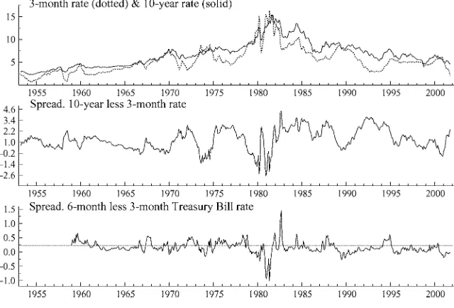
FIGURE1.Time series of monthly interest rates and spreads.

4.1. Results Based on Linear VAR

TABLE1.Testing the expectations hypothesis using VAR’sa

Model/test Results

A. 3- and 6-month rates (s=3 andl=6)

Linear model

Noncausality tests ofSforr(s) 3.53[0.060] Test of term structure restrictions

weak χ2_{(2)=11.16[0.004]}

strong χ2_{(2)=11.38[0.003]}

ρS_,S 0.357

σS/σS 0.552

β 0.197

Linearity tests

VAR vs. 2R-TVAR 68.35[0.007]

VAR vs. 3R-TVAR 92.07[0.036]

2R-TVAR vs. 3R-TVAR 23.73[0.595]

Nonlinear model with two regimes (γ=0.23) Noncausality testsSforr(s)

1st regime 0.439(0.520)[0.570]

2nd regime 0.832(0.356)[0.402]

All 1.269(0.128)[0.128]

ρS_,S 0.189

σS/σS 0.884

β 0.315

B. 3-month and 10-year rates (s=3 andl=120)

Linear model

Noncausality tests ofSforr(s) 3.01[0.083] Test of term structure restrictions

weak χ2_{(2)=5.27[0.072]}

strong χ2_{(2)=4.67[0.097]}

ρS_,S 0.760

σS/σS 0.437

β 0.332

Linearity tests

VAR vs. 2R-TVAR 56.27[0.018]

VAR vs. 3R-TVAR 77.52[<0.001]

2R-TVAR vs. 3R-TVAR 133.79[<0.001]

Nonlinear model with three regimes (γ1= −0.07 andγ2=2.6)

Noncausality tests ofSforr(s)

1st regime 13.53(0.401)[0.359]

2nd regime 2.85(0.266)[0.308]

3rd regime 14.23(<0.000)[0.003]

All 29.31(0.119)[0.164]

TABLE1.(Continued.)

Model/test Results

ρS_,S 0.639

σS/σS 0.766

β 0.489

a_{Sis the theoretical spread andSis the actual;ρis the correlation betweenSandS, andσSandσ} Sare their standard deviations;β=ρσS/σSis the slope. The lag orders of the VAR and TVAR models (selected by SIC) are 1 for both data sets. Some experimentation for the VAR’s indicated that the GNC and cross-equation restriction tests were qualitatively unaffected by settingp=5. Thep-values of the GNC tests for the TVAR’s are calculated using a bootstrap as described in the text: Thep-values given in parenthesis condition on the empirical estimates of the thresholds, whereas those in square brackets permit regime uncertainty.

In summary, the results based on the VAR’s do not support the expectations theory. They match the findings of Hardouvelis (1994) on a similar data set but differ from the results of Campbell and Shiller (1987) for different frequencies and maturities.

4.2. Results Based on TVAR

Table 1 also records the results based on the two- and three-regime TVAR models, as well as tests of the TVARs against the VAR. For both data sets the linear VAR is rejected in favour of the non-linear TVAR.

4.2.1. Three- and six-month interest rates. The tests of the VAR against the 2R-TVAR and the 3R-TVAR both reject at the 5% level, and the specification test of two versus three regimes using heteroskedasticity-corrected p-values finds in favor of the 2R-TVAR. We find ˆγ=0.23, placing 29% of the 169 observations in the upper regime. The estimates of the probabilities of remaining in the same regime, and of switching regimes, are

0.800 0.200 0.510 0.490

,

where the(i,j)element is the probability of being in regime j at timet given that regimei was operative att−1. Thus, there is a more or less equal chance of staying in the upper regime, and switching from the upper to the lower. The tests for GNC fail to reject the null hypothesis in either regime. The correlation (ρ) betweenSandSdecreases relative to the linear model, but the slope coefficient (β) increases becauseσSbetter matchesσS. This is readily apparent in Figure 2, where

comparing the top right panel to the top left one shows the increased dispersion inS from allowing nonlinearity. Otherwise, allowing for nonlinearity has little effect, and the cross plot is no closer to the 45-degree line.

FIGURE2.PredictedSand actual valuesSof the spread: (upper panel) 6- and 3-month rates

Our 2R-TVAR does not entail a similar partitioning of the data, and it seems that there is no short-rate dependence on the size of the spread for this short maturity. The lower panel of Figure 1 plotsStwith a horizontal line drawn at the estimated

threshold value. It is apparent that observations in the 1979–1982 period fall in both regimes.

4.2.2. Three-month and ten-year interest rates. The model specification tests suggest a 3R-TVAR, and that the dynamics of the short rate depend on the sign and size of the spread. The estimated thresholds are−0.07 and 2.6, which places 10% of the observations (19) in the lower regime and 15% in the upper. The empirical transition probabilities are

  

0.684 0.263 0.053 0.042 0.889 0.069

0 0.379 0.621

 

,

implying a longer duration of the middle regime, and an absence of shifts from large spreads (>2.60) to negative ones (<−0.07). The standard deviation of the residuals of the short-rate equation is four times larger in the lower spread regime, at 2.08, than in the upper regime (0.51), while in the middle regime the value is around 1. Although the coefficient of the lagged spread in the short-rate-changes equation is largest (estimated at around 1) in the lower regime, it is not statistically significant, given the large degree of uncertainty that characterizes this regime, as confirmed by the GNC test results presented in Table 1. GNC is only rejected in the upper regime, which is the regime with the smallest residual variance.

The predictions of the changes in the short rate are generated from the 3R-TVAR [to calculateSas in equation (9)] using 1,000 sequences ofk−1 (i.e., 39) forecasts based on bootstrap samples of the residuals. We condition on the full-sample estimates of the coefficients, and use data information up tot−1. We draw from the sub-sample of the full-sample estimated residuals to form the bootstrap samples, where the sub-sample consists of the set of regime-specific residuals warranted by the regime the model is in at that point. We calculate the point forecasts of the changes in the short rate for each one of thek−1 horizons as both the mean and median of the simulated forecast densities. Strictly, the mean is to be preferred because it is the conditional expectation, but the median is more robust to the possibility that a small number of the replications might produce outliers.

The values ofρ, β, and the standard deviationsσSandσSrecorded in Table 1 are

positive relationship is flatter than for the VAR. Comparing results of calculatingS using the means and medians, we find that, for the mean, negative future changes are predicted for intermediate values of the spread, whereas for the median, the predicted changes are positive. The shift upward of the cross plot using the median constitutes stronger evidence in favor of the expectations hypothesis.

We also check the sensitivity of these results to the assumption of a coupon effect. Using the weights without the coupons effect [equation (3)], and the mean of the forecast distribution to obtain point forecasts for each horizon, we calculated S: see Figure 2, bottom right panel. There is a slight shift downward of the cross plot compared to the bottom left panel (with coupon weights), but little substantive difference is noticeable. We also checked the sensitivity of the results to different choices of p(we have hitherto reported results for the SIC-selected p=1 for the VAR’s and TVAR’s), but little difference was observed in the cross plot.

In summary, stronger evidence for the expectations theory results from allowing for non-linearities, especially whenSis relatively large.

5. ECONOMIC ANALYSIS OF THE MODELS

There is a large academic literature on the term structure of interest rates. In this section, we discuss our findings in the light of some of the recent contributions, focusing on the long-maturity-spread case. The implication of the 3R-TVAR is that the spread between the 10-year and the 3-month rates only predicts future changes in the short rate when it is large and positive. We estimated a 3R-TVECM [equation (16)] for this data set (not reported), which indicated that the spread also predictsdecreasinglong rates in the high, positive spread regime, which is at odds with the expectations theory. For example, Campbell (1995, pp. 137–138) found that “[w]hen long rates are unusually high relative to short rates, long rates do not decline to restore the usual yield curve, as one might suppose. Instead long rates tend to rise; the yield spread falls only because short rates rise even faster.”

Thus for high positive values of the spread, our findings are consistent with the puzzle presented in the literature that “the movement of future cumulative short rates obey[s] the overall direction predicted by the expectations hypothesis but at the same time the short-run movement of the long rates does not” [Hardouvelis (1994, p. 256)]. However, for lower values of the spread, future cumulative short rates do not appear to behave as expected either.

already high levels of persistence, would, according to standard models, translate into substantially higher volatility in the long-term rate, a feature of the second half of the 1980’s and 1990’s. Then, small changes in short rates can engineer large changes in long rates, as noted by Campbell (1995, pp. 142–145) in his discussion of the impact of monetary policy on the bond market in the spring of 1994. One strand of argument is that the increased variability of long rates leads to their overreaction to monetary authority policies aimed at preventing the economy from overheating, so that in subsequent periods the disequilibrium between the expected values of the short-term rate and the actual long-term rate leads to decreasing long rates, establishing a negative correlation between the spread and the long rates.4

6. CONCLUSIONS

We show how a threshold VAR of the spread between long- and short-term interest rates and the changes in the short rate arise from a threshold VECM for long and short rates, where the spread is the equilibrium correction term. The threshold nonlinearities can be viewed as resulting from transaction costs, changes in policy regime, time-varying risk premia, etc., and suggest that whether or not the restric-tions imposed by the expectarestric-tions theory may depend on the value of the spread. We consider Granger causality tests of the spread for future changes in the short-rate in the TVAR, and whether allowing for nonlinearity gives a closer match between the actual and theoretical spreads, where the latter is the cumulation of model-based future predicted changes in the short rate.

We show that the dynamics of the short rate and the spread depend on the value of the spread, and that this nonlinear dependence is strong enough to change the results of tests of the expectations theory when the long rate is taken as the 10-year bond interest rate. Then, we find that short rates behave in accordance with the theory when the spread is large and positive. Even then, however, the spread also predicts decreasing long rates. This puzzle has been reported in the literature, but the TVAR model shows that whether the responses to the spread are significant depends on the size of the spread.

NOTES

1. In fact,Γ3has zeros in the last column, so thatrt−3(s)terms are excluded. However, restrictions

of this sort are only valid if the VAR in terms of the two interest rates has exactly the order specified, but because it is only an approximation, we estimate unrestricted VAR’s forr∗t. We illustrate the

cross-equation restrictions implied by the expectations theory for a second-order system. The extension to higher-order VAR’s follows directly.

2. The Markov-switching approach used by Sola and Driffill (1994) has the advantage over the threshold approach that closed-form solutions for multistep predictions are easily obtained, essentially because the Markov-chain state variable is exogenous. However, the exogeneity of the regime-switching process is at the same time a drawback if we wish to model the dependence of the dynamic relationship between the spread and the short rate on the level of the spread directly.

a two-regime model is taken as one of the thresholds of the three-regime model, and a grid search for the second threshold is then conducted. This procedure can be iterated to improve the estimate of the first threshold, and so on. We adopt this procedure for both nonlinear models that we estimate. Bai (1997) proved the consistency of this approach for models with multiple structural breaks.

4. Of course, if policy is credible, the long rate should reflect the expected future low-inflation environment brought about by higher short rates. A time-varying risk premium could be another possible explanation for the negative correlation between the spread and the long-term interest rate. Hardouvelis (1994) finds little support for this, while Tzavalis and Wickens (1998) take the opposite position.

REFERENCES

Anderson, H.M. (1997) Transaction costs and non-linear adjustment towards equilibrium in the US Treasury bill market.Oxford Bulletin of Economics and Statistics59, 465–484.

Bai, J. (1997) Estimating multiple breaks one at a time.Econometric Theory13, 315–352.

Balke, N.S. & T.B. Fomby (1997) Threshold cointegration.International Economic Review38, 627– 645.

Campbell, J.Y. (1995) Some lessons from the yield curve.Journal of Economic Perspectives9, 129–152. Campbell, J.Y. & R.J. Shiller (1987) Cointegration and tests of present value models.Journal of Political

Economy95, 1062–1088.

Clements, M.P. & A.B. Galv˜ao (2001) A Comparison of Tests of Nonlinear Cointegration with an Application to the Predictability of US Interest Rates Using the Term Structure. Mimeo, University of Warwick.

Clements, M.P. & J. Smith (1997) The performance of alternative forecasting methods for SETAR models.International Journal of Forecasting13, 463–475.

Dwyer, G.P., P. Locke, & W. Yu (1996) Index arbritage and nonlinear dynamics between the SP500 futures and cash.Review of Financial Studies9, 301–332.

Enders, W. & C.W.J. Granger (1998) Unit-root tests and asymmetric adjustment with an example using the term structure of interest rates.Journal of Business and Economics Statistics16, 304–311. Ericsson, N.R. & J. Marquez (1998) A framework for economic forecasting.Econometrics Journal1,

C228–C266.

Granger, C.W.J. & T. Ter¨asvirta (1993)Modelling Nonlinear Economic Relationships. Oxford: Oxford University Press.

Gray, S.F. (1996) Modeling the conditional distribution of interest rates as a regime-switching process.

Journal of Financial Economics42, 27–62.

Hall, A.D., H.M. Anderson, & C.W.J. Granger (1992) A cointegration analysis of Treasury bill yields.

Review of Economics and Statistics74, 116–126.

Hamilton, J.D. (1988) Rational-expectations econometric analysis of changes in regime. An inves-tigation of the term structure of interest rates.Journal of Economics, Dynamics and Control12, 385–423.

Hansen, B.E. (1996) Inference when a nuisance parameter is not identified under the null hypothesis.

Econometrica64, 413–430.

Hansen, B.E. (2000) Testing for linearity. In D.A.R. George, L. Oxley, & S. Potter (eds.),Surveys in

Economic Dynamics, pp. 47–72. Oxford: Blackwell.

Hansen, B.E. & B. Seo (2001) (in press). Testing for two-regime threshold cointegration in vector error correction models.Journal of Econometrics.

Hardouvelis, G.A. (1994) The term structure spread and future changes in long and short rates in the G7 countries.Journal of Monetary Economics33, 255–283.

Mankiw, N.G. & J.A. Miron (1986) The changing behaviour of the term structure of interest rates.

Quarterly Journal of Economics101, 211–228.

Pagan, A.R., A.D. Hall, & V. Martin (1996) Modelling the term structure. In G.S. Maddala & C.R. Rao (eds.),Handbook of Statistics, Statistical Methods in FinanceVol. 14: pp. 91–118. Amsterdam: North-Holland.

Pfann, G.A., P.C. Schotman, & R. Tschernig (1996) Nonlinear interest rate dynamics and implications for the term structure.Journal of Econometrics74, 149–176.

Roberds, W., D. Runkle, & C.H. Whiteman (1996) A daily view of yield spreads and short-term interest rate movements.Journal of Money, Credit and Banking28, 34–53.

Rudebusch, G.D. (1995) Federal reserve interest rate targetting, rational expectations, and the term structure.Journal of Monetary Economics35, 245–174.

Sola, M. & J. Driffill (1994) Testing the term structure of interest rates using a stationary vector autoregression with regime switching.Journal of Economic Dynamics and Control18, 601–628. Tsay, R.S. (1998) Testing and modeling multivariate threshold models.Journal of the American

Sta-tistical Association93, 1188–1202.

Tzavalis, E. & M. Wickens (1998) A re-examination of the rational expectations hypothesis of the term structure: Reconciling the evidence from long-run and short-run tests.International Journal of

Finance and Economics3, 229–239.

van Dijk, D. (1999)Smooth Transition Models: Extensions and Outlier Robust Inference. Ph.D. Dissertation, Tinbergen Institute.

van Dijk, D. & P.H. Franses (2000) Nonlinear error-correction models for interest rates in the Netherlands. In W.A. Barnett, D.F. Hendry, S. Hylleberg, T. Ter¨asvirta, D. Tjostheim, & A. Wurtz (eds.),Nonlinear Econometric Modelling in Time Series: Proceedings of the Eleventh International

Symposium in Economic Theory. Cambridge, UK: Cambridge University Press.

Watson, M.W. (1999) Explaining the increased variability in long-term interest rates.Federal Reserve

Bank of Richmond, Economic Quarterly85, 71–96.

APPENDIX A

To evaluate the RHS of (10), note that

Et−1rt+j(1)=irEt−1Rt+j =ir

C j

s=0

Γs_+Γj+1_R

t−1

so that the RHS of (10) can be written as (omittingθ):

1 k

_k−1

i=1

i

j=1

Et−1rt+j(1)

= 1

kir k−1

j=1

(k−j)

C j

s=0

Γs+Γj+1Rt−1

.

If we focus solely on the term inRt−1,

1 kir

k−1

j=1

(k− j)Γj+1

Rt−1=irΓ2(I−Γ)−1(I−Γk−1)Rt−1−

1 kirΓ

k−1

j=1

jΓj Rt−1.

For largek, the term inRt−1is approximatelyirΓ2(I−Γ)−1Rt−1, becauseΓk−1 0, and

jΓj+1_→

APPENDIX B

Writing the elements ofΓ1andΓ2defined in (7) as

Γ1=

_ϕ

11 ϕ12

ϕ21 ϕ22

, Γ2=

_θ

11 θ12

θ21 θ22

(whenp=2), the cross-equation restrictions implied by equation (13) for the VAR of the spread and the short rate whenk=2 are

ϕ11(2−ϕ21)=ϕ22ϕ21+θ21

ϕ12(2−ϕ21)=ϕ22ϕ22+θ22

θ11(2−ϕ21)=ϕ22θ21

θ12(2−ϕ21)=ϕ22θ22.

When the stronger version of the theory is employed, the restrictions are

ϕ21=2, ϕ22=0, θ21=0, θ22=0

Fork= ∞, the restrictions given by equation (11) are

ϕ11(1−ϕ11−ϕ21)=ϕ22ϕ21+ϕ12ϕ21+θ11+θ21,

ϕ12(1−ϕ11−ϕ21)=ϕ22ϕ22+ϕ12ϕ22+θ22+θ12,

θ11(1−ϕ11−ϕ21)=ϕ22θ21+ϕ12θ21,

θ12(1−ϕ11−ϕ21)=ϕ22θ22+ϕ12θ22,

and for the stronger version,

1−ϕ11=ϕ21

−ϕ12=ϕ22

θ11+θ21=0