The implementation of the Arbitrary Lagrangian Eulerian method into a FEM Discontinues Galerkin Solver

(1)

Internship Report - San Diego State University

The implementation of the Arbitrary Lagrangian Eulerian method into a FEM - Discontinues Galerkin Solver

Mentor: Prof.Dr.Ir. Gustaaf Jacobs Supervisor: Prod.Dr.Ir. H.W.M. Hoeijmakers

Period: 1 feb - 31 may 2012

Sunny S. Titus (s0174181) Engineering Fluid Dynamics University of Twente , The Netherlands

[email protected]

(2)

Abstract

The main objective of this paper is to test the performance of the Arbitrary Eulerian-Lagrangian method implemented into a Discontinuous Galerkin-FEM solver. H- and p-convergence test are performed to assess if the implementation full fills the expected convergence rate. The validation cases performed are the stationary inviscid vortex in a moving domain and

Stokes 2nd problem. As an extra case the oscillation of a cylinder in an uniform flow is examined. No exact solution exists of this problem thus a

(3)

Acknowledgements

First of all i want to thank professor Guus Jacobs. Without him I would have missed th wonderful experience of visiting the United States. He introduced me into the wonderful world of CFD. His positive attitude, his willing to help nature and his love for soccer made me feel right at home.

I would like to thank my family, whoms regular skype conversations and texts made me feel like i never left home. Thank you for always being there for me.

I would like to thank Sonia and Daniel Nelson. Who gave me a place to stay and treated me like family from the first day we met to the day we said our goodbyes.

I would like to thank Sean Davis who helped me explore pacific beach and provided me regularly with a place to stay.

(4)

Introduction

Many practical applications for fluid problems, such as the extension of aircraft flaps, the scour beneath offshore pipelines or fluid-structure interac-tion, depend on time varying domains. The Arbitrary Lagrangian Eulerian (ALE) method is used in this paper to cope with these kind of problems.

The ALE method uses a mapping between the physical time-varying domain and the stationary reference domain. By transforming the conser-vation laws using this mapping we are able to solve the time varying domain on a stationary grid.

The transformed conservation laws are solved in space using the Discon-tinuous Galerkin method. This method is a higher order numerical method which combines FEM’s higher order elements with the FVM’s locality. The time integration which will be used is a 4th order Runge-Kuta scheme.

The objective of this work is to investigate the performance of the ALE-method implementation in a DGM framework. In the first section of chapter 2 the Navier-Stokes equations are discussed and the non-dimensioless form is given. The ALE-method is presented in the next section. The mapping between the domains will be discussed and the transformation of the con-servation laws from the physical to the reference domain will be presented. In the last section of Chapter 2 the general idea of DG-method is explained. We will look at the derivation of the weak form, introduce the reference element as a way to efficiently derive the mass and stiffness matrices, talk about the numerical flux and finally we discuss the need for a good node distribution inside the elements.

(6)

(7)

Chapter 2

Formulas and theorems

In this chapter we will introduce the governing equation and derive its non-dimensional form. In the next section the ALE-method will be explained, introducing the reference domain the transformed NS-equations and its re-lation to moving boundaries. In the last section we will look at the DG-method and discuss its basic properties and assumptions. The result will be a fully functional DG-method for solving the NS-equations in a domain with moving boundaries.

2.1 Governing Equations

The equations used in the CFD code are the 2D Euler and Navier-Stokes equations. In equation 2.1 the conserved vector form of the Navier-Stokes equations is displayed. Neglecting the viscous terms results in the Euler equations. It is assumed that the kinematic viscosity is independent of density and temperature and is homogeneous in space and time.

~

Qt+F~xinv+G~yinv =F~xvis+G~visy (2.1)

Where Q is the vector of conserved variables, F the vector containing the fluxes in the x-direction andGthe vector containing the fluxes in y-direction. These vectors are fully defined in equation 2.2.

Q=        ρ ρu ρv E       

, ~Finv =        ρu ρu2+p

ρvu

(E+p)u

      

, ~Ginv =        ρv ρuv ρv2+p

(E+p)v

       (2.2) ~ Fvis=

       0 τ11 τ12

τ13−qx

      

, ~Gvis=        0 τ21 τ22

τ23−qy

(8)

Whereτ is the stress tensor, defined by:

τ11= µ 2ux−2₃(ux+vy)

τ12=τ21= µ(uy+vx)

τ13= µ 2vy−2₃(ux+vy)

τ22= uτ11+vτ12

τ23= uτ21+vτ22

And the heat conduction is given by Fouriers law:

qx =−κTx; qy =−κTy

At this point there are only 5 equations for the 7 unknowns. To solve this it is assumed that the fluid acts like an ideal gas. Therefore the perfect gas law is added to the set of equations:

P = RT

ρ

The last equation is that of the internal energy. The total energy is defined by the sum of the internal energy and the kinetic energy:

E =ρe+ρ 2 u

2₊_v2

The internal energy for an ideal gas is given bye=CVT and, because the

gas is ideal, the heat capacity is given by CV = _γR−1 =

P

ρT(γ−1). Therefore the total energy becomes as is displayed in equation 2.3 and and a fully defined set of equations is obtained:

E= P

γ−1+

ρ

2 u 2₊_v2

(2.3)

2.1.1 Dimensionless equations

To easily adjust the flow parameters it is more convenient to work with dimensionless variables. To make the equations dimensionless the following dimensionless variables are defined in equation 2.4 , where the superscript * stands for a dimensional variable and the subscript f refers to a reference variable:

ρ= ρ_ρ∗∗

f u=

u∗

U∗

f v=

v∗

U∗

f

T = T_T∗∗

f P =

P∗ ρ∗

fU

∗

f

2 µ=

µ∗ µ∗_f

x= _Lx∗∗

f y=

y∗

L∗

f t=

t∗U_f∗ L∗

f

(2.4)

(9)

Prandtl and Mach number as parameters. These equations are displayed in 2.5 where the vectors are fully defined in 2.6.

~

Qt+F~xinv+G~invy =

1

Ref

~

F_xvis+G~vis_y (2.5)

Q=        ρ ρu ρv E       

, ~Finv =        ρu ρu2+p

ρvu

(E+p)u

      

, ~Ginv =        ρv ρuv ρv2₊_p (E+p)v

       (2.6) ~ Fvid =

         0 τ11 τ12

τ13+₍_γ₋₁₎1_M2

fP r

Tx         

, ~Gvid =          0 τ21 τ22

τ23+₍_γ₋₁₎1_M2

fP r

Ty         

The speed of sound, the Reynolds, the Prandtl and the Mach number are defined as:

Ref =

U_f∗L∗_fρ∗_f µ∗

f P r=

Cp∗µ∗

κ∗

Mf = U_f∗

c∗ c∗ =

q

γR∗_T∗

f =

r

γP ∗

f

ρ∗_f

2.2 Arbitrary Langrangian Eulerian Method

(10)

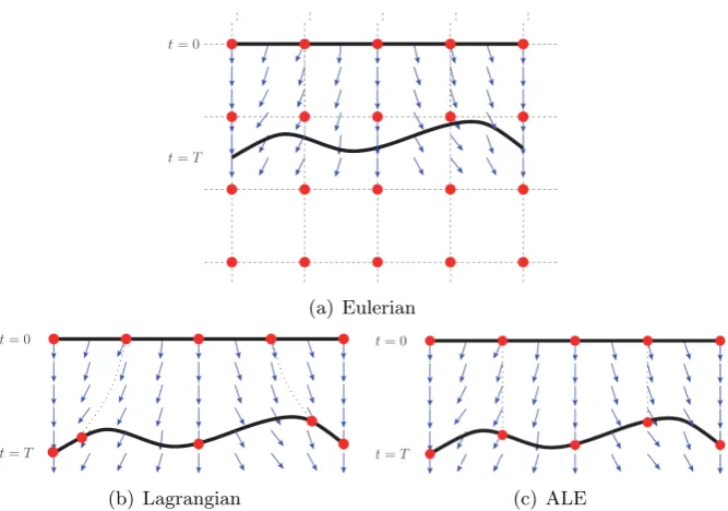
(a) Eulerian

[image:10.595.131.465.123.357.2]

(b) Lagrangian (c) ALE

Figure 2.1: Different reference frames

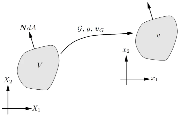
The ALE method in this report is based on Per-Olof Persson’s paper [1]. The essence of the ALE method is to transform the physical domain, con-taining the moving boundaries, to a fixed grid domain where the equations can be solved with more ease using existing methods. This is schematically displayed in figure 2.2. To do this a mapping function ~x =G(χ~) needs to be declared which transforms the reference state coordinates to the physical state coordinates. This mapping function can be a function of the forces in the system (e.g. to simulate the change of a boundary due the forces exerted on it) or, as is the case in this report, the mapping function can be prescribed. We assume that the mappings function is a smooth one-on-one function. To successfully transform the Navier-Stokes equation from the physical domain to the reference domain, three more properties of the mapping function are needed. The mapping deformation gradient G, its determinantg and the mapping velocity vχ.

G=∇χG, vχ= ∂_∂tG

χ g=det(G)

With these transformation properties it is possible to find the relation between the infinitesimal strain of an edge in physical domain and that of its reference domain counterpart through:

dl=GdL

(11)

[image:11.595.118.477.124.369.2]

Figure 2.2: Mapping between the physical and the reference domains

which is related to its reference domain counterpart through:

v=gdV

At last the infinitesimal area change in the reference and physical domain are defined by:

dA=NdA; da=nda

Combining these definitions results into the relationship between the infinitesimal area change in the physical and reference domain:

dl·nda=gG−1dl·N dA

nda=gG−TNdA (2.7)

(12)

Z

v(t)

∂Q

∂t dv+

Z

v(t)

∇ ·Fdv= 0 (2.9)

Applying the divergence theorem to equation 2.9 results in: Z

v(t)

∂Q

∂t dv+

Z

∂v(t)

F·nda= 0 (2.10)

The first part of equation 2.10 will be evaluated first. Applying the Leibniz integral rule and substituting equation 2.7 results in:

Z

v(t)

∂Q

∂tdv = d dt

Z

v(t)

Qdv−

Z

∂v

(Qvg)·nda

= d

dt

Z

V

QgdV −

Z

∂V

(Qvg)· gG−TN

dA

= Z

V

∂(gQ)

∂t χ dV − Z ∂V

gQG−1vg

·NdA

The second part is also transformed using equation 2.7 : Z

∂v

F·nda= Z

∂V

F· gG−TN

dA= Z

∂V

gG−1F

·NdA

Combining the two parts results in the transformed Navier-Stokes equa-tions:

Z

V

∂(gQ)

∂t χ dV + Z ∂V

gG−1F−gQG−1vg

·NdA= 0

Which can be written in partial differential form:

∂(gQ)

∂t

_χ

+∇_χ gG−1F−gQG−1vg

= 0

∂Q_χ

∂t χ

+∇χ.F Qχ,∇χQχ

(13)

For the transformed Fluxes and conserved quantities in the reference domain the following equations apply:

Q_χ=gQ, Fχ=gG−1F−QχG−1vχ

In the above equations the subscript χ indicates that variables and op-erators are only valid in the reference space. The absence of this subscript refers to the operators and variables in the physical space.

When the transformed NS-equations are written as a system of 1st order equations we obtain:

∂Q_χ

∂t

χ

+∇_χ.F Q_χ, Uχ

= 0 (2.11)

Uχ− ∇χQχ= 0

The variable Uχ is however only valid in the reference space while the

equation to obtain the reference fluxes needs the physical fluxes as input. To construct the physical fluxes we therefore first need to transform this variable to the physical domain. This can be done by using the chain rule:

∇Q=G−T g−1∇_χQ_χ−Q_χ∇_χ g−1

=G−T g−1Uχ−Qχ∇χ g−1

At this point the transformed NS-equations in partial differential form is fully defined and ready to use. All the calculation in the CFD code take place in the reference domain using the transformed NS-equations where after the result will be mapped to the physical domain. In the physical domain the physical fluxes are computed and transformed to the reference fluxes. The reference fluxes are then used for computation in the reference domain and the circle starts again.

2.3 Discontinues Galerkin Method

For the spatial discretization the discontinues Galerkin method is used. To derive the DG-method we multiply the transformed Navier-Stokes equations 2.11 with a test functionφand integrate it over space. To keep the equations easy to read the subscripts are dropped.

Z

V

∂Q

∂tφdV +

Z

V

∇.FφdV = 0

Applying the product rule on the second term results in: Z

V

∂Q

∂tφdV −

Z

V

F· ∇φdV =−

Z

V

(14)

Using the divergence theorem this becomes: Z

V

∂Q

∂tφdV −

Z

V

F· ∇φdV =−

Z

∂V

N·(F∗φ)dV

Z

V

∂Q

∂t φdV −

Z

V

F∂φ ∂xdV −

Z

V

G∂φ

∂ydV =−

Z

∂V

NxF∗φdV −

Z

∂V

NyG∗φdV

(2.12)

Where F∗ is the boundary flux and the flux vector is defined as F= F G .

2.3.1 Reference element

Now lets divide the domain in K elements which creates a structured or unstructured mesh. The integral derived above is also valid for each ele-ment.The local solution of the conserved variables, the fluxes and the test functions all can be described by an Lagrange polynomial:

Q=

Np

X

i=1

Qi(xi, t)li(x) ; F= Np

X

i=1

Fi(xi, t)

Gi(xi, t)

li(x) ; φ= Np

X

i=1

φi(xi, t)li(x)

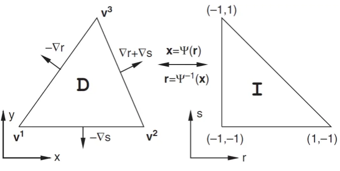
However, because we are working with triangle elements in (un)structured mesh, the orientation and size of the elements may differ from each other. In-stead of finding basis functions for each elements we transform the elements to a reference triangle, displayed in figure 2.3.1. For this reference triangle we only have to find the basis functions once which can be transformed back to each random triangle.

Q=

Np

X

i=1

Qi(ri, t)li(r) ; F= Np

X

i=1

Fi(ri, t)

Gi(ri, t)

li(r) ; φ= Np

X

i=1

φi(ri, t)li(r)

Now lets apply the integral equation 2.12 upon the reference element and substituting the polynomial representation of conserved variables,fluxes and test function into the equation 2.12. After collecting all the terms into matrices and vectors and keeping in mind that the variables Qi,Fi and φi

aren’t functions of space any more,the equation can be rewritten to: Z

V

[m]dV∂Q ∂t −

Z

V

[sx]dVF−

Z

V

[sy]dVG=−

Z

∂V

[medge,x]∂V NxF∗−

Z

∂V

(15)

[image:15.595.128.467.133.304.2]

Figure 2.3: Mapping between a random element and the reference element

Where [m],[sx],[sy],[mxedge] and [myedge] are given by:

mij =lilj; sx,ij =li∂l_∂xj; sy,ij =li∂l_∂yj;

mxedge=lilj; myedge=lilj;

This can be further simplified by taking the integrals inside the matrices:

[M]∂Q

∂t −[Sx]F−[Sy]G=−

h

M_xedgeiNyF∗−

h

M_yedgeiNyG∗

And after some rearrangement this finally results in:

∂Q

∂t = [Sx] [M]

−1_F_+[_S

y] [M]−1G−

h

M_xedgei[M]−1NxF∗−

h

M_yedgei[M]−1NyG∗

Where the matrices are given by:

Mij =

R

V liljdV Sx,ij =

R

V li ∂lj

∂xdV Sy,ij =

R

V li ∂lj

∂ydV

M_x,ijedge=R

∂V lilj∂V M edge y,ij =

R

∂V lilj∂V

2.3.2 Flux function

(16)

is very dissipative, it will produce good results in smooth (no discontinuities) flows. The flux is defined as:

(N xF+N yG)∗ =N x{{F(Q)}}+N y{{G(Q)}}+C 2JQK

The first and second terms on the right hand side are the average fluxes across the boundary defined by:

{{F}}= F

+₊_F−

2 The third term is a jump term along a normal:

JQK=N

−_Q−₊_N+_Q+

The last unknown is the constant C which is the maximum eigenvalue of the matrix

N x∂F ∂Q+N y

∂G

∂Q

2.3.3 Legendre-Gauss-Lobatto quadrature

At this point we have rewritten the conservation laws into a system of equa-tions of which the flux funcequa-tions are fully defined. The only things still unknown are the mass and stiffness matrices which depend upon the inte-gration of the Lagrangian interpolation polynomials.To compute the integral of these matrices Gaussian quadrature (2.13) is used . This numerical inte-gration method will produce exact results for polynomials of order 2n−1 and a suitable choice of the points xi and weights wi. A type of

polyno-mial that is often used in combination with the Gaussian quadrature is the Legendre polynomial which possess the following property :

R

liljdx= 0 f or i6=j

The Legendre polynomial can be created on the fly by using Bonnets recur-sion formula and after determining its roots, the weights are easily deter-mined using equation 2.14. A disadvantages is however that the integration points don’t include the grid points that span the element on which usu-ally B.C. are applied. To solve this Legendre-Gauss-Lobatto quadrature is applied combining the high accuracy of the Gaussian quadrature, the or-thogonality of the Legendre polynomial and including the end points of the integration domain as described by Lobatto.

Z 1

−1

f(x)≈

n

X

i=1

wif(xi) (2.13)

wi=

2

1−x2_i[P_n0 (xi)]2

(17)

Jan Hesthaven’s book [3] provides us with algorithms to determine the Van der Monde matrixV, its gradient (VR, Vs) and the transformation

gra-dientJk. The Jacobian is used to transform the reference element matrices back to the original elements.

Vr= _drdl

ri Vs =

dl ds

si

DrV =Vr DsV =Vs

Sx = ∂r_∂xDr+_∂x∂sDs Sy = ∂r_∂yDr+∂s_∂yDs

Mk=Jk V VT−1

(2.15)

2.4 Summary

(18)

Chapter 3

Numerical Results

In the previous chapter I discussed the dimensionless Euler/NS-equations, the ALE-method and the DG-method. In this chapter the implementation of the ALE method into the DG-solver is examined using several test cases and mappings. For each of the test cases an exact solutions exists and the

L2 norm can be determined. A p- and h-refinement study will be performed to validate our implementation of the ALE-method. As a ’bonus’ case the flow about a oscillating cylinder is presented. An exact solution for this problem doesn’t exist, however validation is sought in comparing its lift and drag coefficients to those found in literature.

3.1 Test case 1 - Moving vortex using the

Euler-equations

The exact solution for the moving vortex problem is based on the potential flow theory and its velocity solution is given in the paper .... In the same paper an exact solution for the density field is provided and, because the flow is isentropic, the pressure field obeys the equationP =P(ρ). The exact solution is displayed in equation 3.1 ,whereβrepresents the vortex strength,

x0 and y0 the original vortex coordinates andu0 and v0 the velocity of the vortex. Further the heat capacity ratio is given byγ, the density byρ , the x- and y-velocity byuand vand the pressure byP. The radiusr is defined in equation 3.2.

ρ=

1−(γ−1)β

2_exp₍₂₍₁₋_r2₎₎

16γπ2

_γ₋1₁

u=u0−βexp 1−r2

(y−yo−vot)

2π

v=v0−βexp 1−r2

(x−xo−uot)

2π

P =ργ

(19)

r = q

(x−x0−ut)2+ (y−y0−vt)2 (3.2) The ALE implementation is tested using p- and h-convergence test, with the polynomial order ranging from order 2 to 5 and the grid size from 2 to 0.25.For the boundary conditions and the initial conditions the exact solu-tion is used.

The mapping-function is used to test the correct implementation of both the deformation matrixGand the deformation velocityvg. It starts with a 1

on 1 mapping gradually transforming in the defomermed grid as is sidplayed in Figure... The mappings-function, deformation matrix and mappings ve-locity are:

~ x=

X+ sin ₁₀πX

sin ₁₀π [Y + 5] sinπt Y + sin (X) sin ₁₀π [Y + 5]sin (πt)

(3.3)

[G] =

1 + ₁₀π

cos ₁₀πX

sin ₁₀π [Y + 5]

sinπt ₁₀π

sin ₁₀πX

cos ₁₀π [Y + 5] sinπt

cos (X) sin ₁₀π [Y + 5]sin (πt) 1 + ₁₀πsin (X) cos ₁₀π [Y + 5]sin (πt)

(3.4) vg=

πsin ₁₀πX

sin ₁₀π [Y + 5]

cos (πt)

πsin (X) sin ₁₀π [Y + 5]cos (πt)

(3.5)

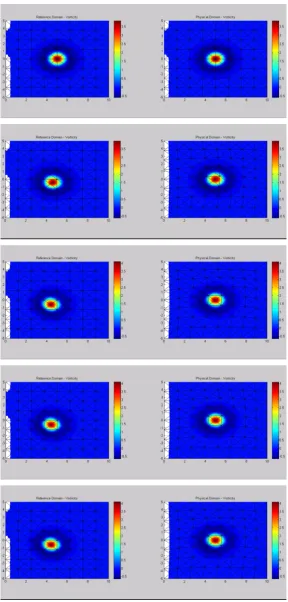
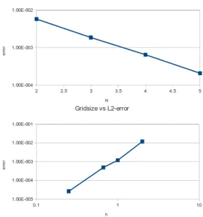
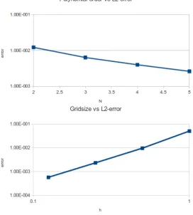
Figure 3.1 shows the result of the stationary votex in a moving domain. The right domains are the moving physical domain. The left domains are the stationary reference domain. We notice that for the vortex to remain stationary in the physical domain it has to compensate for the movement of the grid, which is visable in the reference domain where the vortex is avected in the opposite direction as the map deformation in the physical domain. In Figure 3.2 the h- and p-convergence test of the vortex in the physical domain att = 2 are displayed. The p-test is performed on a domain with gridsize

h = 2. The numerical error of the DG-method is of the ordere= O hP, which can b rewritten to log(e) = 1/hP = 1/2P. In Figure 3.2 we indeed observe that the error reduces 1 order if we increases the polynomial order with 2. For the h-test we used a polynomial order of P = 3. by rewriting the error to log(e) = log(hP) = P log(h) we expect to a slope of 3. In Figure 3.2 we indeed notice that for each order h decreases the order of the error decreases with 3.

3.2 Test case 2 - Stokes 2nd problem

Stokes 2ndproblem is used to verify the ALE implementation for the Navier-Stokes equations. The problem consist of a infinite moving plate that os-cilattes according:

(20)

[image:20.595.153.442.123.727.2]

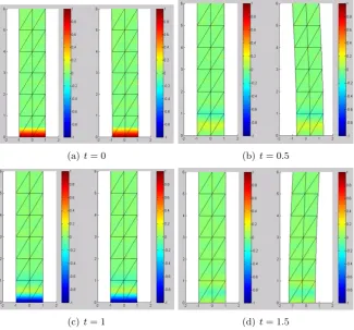
Figure 3.1: A stationary vortex in a moving domain at various timesteps. The domains at the left are the reference domains, the domains at the right

(21)

[image:21.595.150.442.254.567.2]

(22)

[image:22.595.151.445.123.299.2]

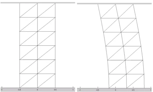
Figure 3.3: The fixed top moving wall deformation used in Stokes 2nd prob-lem. On the left the initial state. On the right the state att= 0.5.

By making the assumptions that the flow is incompressible, uni-directional parralel to the plate and the Reynolds number is small such that we have a laminair flow an exact solution can be derived:

u(y, t) =U0e−

√

ωRe/2y_{cos (}_ωt₋_ωRe/₂_y₎ _(3.7)

To simulate stokes 2nd problem we use rectangular domain on which in the x and y direction periodic boundary conditions are applied. At the top zero velocity is enforced while at the bottom the plate velocity is imposed. The mapping for this problem is described by:

~ x=

X+ U0

ω sin (ωt) cos Y

6π/2

Y

(3.8)

[G] =

1 −U0

ω sin (ωt) sin Y

6π/2 ₁

6π/2 0 1

(3.9)

vg=

U0cos (ωt) cos Y₆π/2

0

(3.10)

(23)

(a)t= 0 (b) t= 0.5

[image:23.595.135.461.219.522.2]

(c)t= 1 (d) t= 1.5

(24)

[image:24.595.161.434.264.567.2]

(25)

3.3 Test case 3 - Oscillating cylinder in uniform

flow

For the oscillating in an uniform flow no analytical solutions do exists. To verify that our implementation does work we look at the lift and drag co-efficients created by the movement of the cylinder and compare it with the results of Perrson’s work. His results are displayed in Figure 3.7 . The mapping used is a blended mapping. By blending a rigid mapping with a stationary mapping a part of the domain can be deformed. In our case the part surrounding the cyllinder. This is achieved by declaring a point

~

XC and the distance Rc form this point from which we want the

map-ping to be rigid. The distance from this region can be measured using

d

~ X

= ||X~ −X~C|| −Rc. The next step is to declare the region that

re-mains stationary. This is done by choosing a distance D with respect the rigid motion region. if the ratio d/D < 0 a point lays in the rigid motion area. If the ratio d/D >1 a point lays in th stationary domain. Anything else means the mapping is a combination of both the stationary mapping as the rigid motion mapping. The mapping is given by:

~

x=b(d(~x))X~ + (1−b(d(~x)))Y~

~ X

, (3.11)

with the blending function b:

b(d) =  



0, if d <0

1, if d > D

r(d/D), otherwise.

(3.12)

The blending polynomialr used is:

(26)

(a)t= 6.0 (b) t= 6.5

[image:26.595.115.480.123.773.2]

(c)t= 7.0 (d) t= 7.5

Figure 3.6: The x-velocity of a cyllinder oscilatting in a uniform flow at various times. The top images are the reference domains and the bottom

(27)

[image:27.595.122.471.176.325.2]

Figure 3.7: The lift and drag coefficient created by the moving cyllinder in an uniform flow. Taken from Perrson’s paper.

[image:27.595.208.386.468.638.2]

(28)

Chapter 4

Conclusion

Th objective of this paper is to implement the Arbitrary-Eulerian method into a Discontinuous Galerkin Solver and test its performance. This has been done by considering 3 test cases.

For the first case, the stationary vortex problem in a deforming domain, both the h- and p-test fulfilled our expectations. We therefore can con-clude that the implementation of the ALE-method in combination with a DG-solver provides us with high order method to solve moving boundary problems in the case of the Euler-equations.

The second case, Stokes 2nd problem for which the top is fixed and the bottom wall oscillates, both the h- and p-test fulfilled our expectations. However the mapping for this problem is rather simple. The term ∇~g−1 for this mapping equals zero and therefore has not been tested. We do conclude that for simple mappings for which a constant determinant g of the deformation matrix [G] applies does work and provides us with high order method to solve moving boundary problems in the case of the Navier-Stokes equations.

The last case, the oscillating cylinder in an uniform flow, has no exact solution thus no conclusions can be deducted. However comparing it with the solution found by Persson we do find the same shape for the lift and drag coefficients in time.

Futher work

To fully verify the implementation works in combination with the Navier-Stokes equations a mapping need to be tested of which the determinant is a function of the space.

Further the effect of the geometric conservation law has been ignored for this study while in the paper of Persson he describes that the effect can become rather large for low order elements.

(29)

should be implemented into a numerical solver written in a faster language like C or fortran.

(30)