Improved capacitive readout for a Coriolis mass flow sensor

(1)

1

Faculty of Electrical Engineering,

Mathematics & Computer Science

Improved Capacitive Readout for a

Coriolis Mass Flow Sensor

Liufei Yang B.Sc. Thesis

July 2018

Supervisors:

(2)

(3)

Abstract

Most of the MEMS-based (Micro Electro Mechanical System) flow sensors operate using the thermal measurement principle. A disadvantage of thermal-based mea-surement techniques is that they need to be calibrated for each specific fluid. This is not necessary for Coriolis mass flow sensors, which offer a way to directly measure the mass flow.

A microfabricated Coriolis mass flow sensor was developed by Enoksson et al. in 1997. Multiple improvements were made to the sensor over the years, but the method for reading out the measurements remained unchanged for a long time. In 2015, Alveringh et al. proposed a novel detection principle for reading out the Coriolis mass flow sensor which is able increase the sensitivity of the sensor. This research is based on the method developed by Alveringh et al. and focuses on characterizing the increase in the sensitivity of the sensor.

The Coriolis mass flow sensor has two outputs, and the phase shift between the two outputs provides a measure of the mass flow. The detection principle developed by Alveringh et al. partially cancels a component of the output signals so that a larger phase shift is detected. A mathematical model for the change in sensitivity with respect to the cancellation is derived.

The change in phase is measured for different flow rates and different amounts of cancellation. The results show a very strong linear relationship between the flow rate and change in phase. The sensitivity at each cancellation level is defined as the the change in phase with respect to flow rate, i.e. the gradient. The sensitivity increases as the amount of cancellation increases, which is in accordance with the theory. However, there is some discrepancy with the mathematical model, which predicted a faster increase in sensitivity with respect to the cancellation. This is presumably due to a variety of idealized assumptions made in the mathematical model. The results of this experiment demonstrate that the detection principle developed by Alveringh et al. does in fact produce a significant increase in sensitivity, but the mathematical model for quantifying this increase needs to be made more precise.

(4)

(5)

Introduction

Most of the MEMS-based (Micro Electro Mechanical System) flow sensors operate using the thermal measurement principle [1]. There are different implementations, for example, a heated probe can be inserted into the fluid and the amount of energy required to keep the temperature of the probe constant can be measured [2]. This energy will be related to the mass flow.

A disadvantage of thermal-based measurement techniques is that they need to be calibrated for each specific fluid. This is not necessary for Coriolis mass flow sensors, which offer a way to directly measure the mass flow. Thus, Coriolis mass flow sensors have a distinct advantage in that they are able to take measurements of mass flow which are independent of fluid properties, which may not always be known.

A microfabricated Coriolis mass flow sensor was developed by Enoksson et al. in 1997. Multiple improvements were made to the sensor over the years, but the method for reading out the measurements remained unchanged for a long time. In 2015, Alveringh et al. proposed a novel detection principle for reading out the Coriolis mass flow sensor which is able to increase the sensitivity of the sensor [3]. This research is based on the method developed by Alveringh et al. and focuses on characterizing the increase in the sensitivity of the sensor.

(8)

(9)

Chapter 2

Theory and Mathematical Model

2.1 Principle of Operation

The Coriolis force is an inertial force that arises when objects are moving in a rotating frame of reference [4]. Due to the rotation, an object that moves in a straight line will appear to follow a curved path when observed from the inertial frame. The force that seemingly deflects the object is called the Coriolis force, and the deflection of an object due to the Coriolis force is known as the Coriolis effect.

A Coriolis mass flow sensor relies on the Coriolis effect for its operation. As illustrated in Figure 2.1, the main part of the sensor consists of a tube that follows a square path. This tube is in a magnetic field, so when an alternating electric current is run through a metal layer on top of the tube, the resulting Lorentz force will cause the tube to vibrate [5]. The vibration due to the actuation is known as the ”twist mode” of the sensor and is indicated byω.

When a fluid is allowed to flow in the tube, the mass flowΦmwill induce a Coriolis forceFcbecause the twist mode forces the fluid to change velocity. The Coriolis force is given by

⃗

Fc=−2L⃗ω×Φ⃗m (2.1)

[image:9.595.214.412.623.739.2]

The Coriolis force causes the tube to swing, and the ratio between the swing mode

Figure 2.1: Coriolis mass flow sensor. Figure taken from [6].

(10)

[image:10.595.113.450.88.209.2]

Figure 2.2: Illustration of the twist mode due to the actuation (left) and the swing mode due to the Coriolis force (right). Figure taken from [7].

vibration amplitude and the twist mode vibration amplitude is proportional to the mass flow. An illustration of the swing mode and twist mode vibration is shown in Figure 2.2. The ratio between the vibration amplitudes can be determined by mea-suring the phase shift between two capacitive readout structures placed on opposite sides of the rotation axis of the twist mode [3]. This will be further explained in the next section.

2.2 Sensor Readout

[image:10.595.79.501.556.666.2]

The conventional readout of the Coriolis mass flow sensor is achieved using ca-pacitive comb structures on either side of the rotation axis of the twist mode. A high-frequency MHz carrier signal is connected to each capacitive comb, and the comb outputs are connected to charge amplifiers to transform the capacitance to a voltage. This is illustrated in Figure 2.3.

Figure 2.3: Schematic of readout electronics. Figure adapted from [5].

The transfer function of the charge amplifier circuit is given by

uout=−

Cr

Cf

(11)

2.2. SENSORREADOUT 5

whereCr is the readout capacitance,Cf is the feedback capacitance,uinis the input voltage, anduoutis the output voltage [7]. The input voltage in this case is the carrier signal. Thus, the output signal of the charge amplifier will be proportional to the amplitude of the carrier signal.

[image:11.595.149.480.292.530.2]

The signal in each of the capacitive readouts is composed of a component due to the twist mode of the sensor and a component due to the swing mode of the sensor, as illustrated in Figure 2.4. These will be referred to as the actuation mode signal and the Coriolis mode signal respectively. The actuation mode signal is proportional to the number of finger pairs in the capacitive comb as well as the distance of the comb from the center of the sensor. The Coriolis mode signal is only proportional to the number of finger pairs [3].

Figure 2.4: Conventional readout of the Coriolis mass flow sensor. Figure taken from [3].

(12)

2.3 Mathematical Model of Cancellation

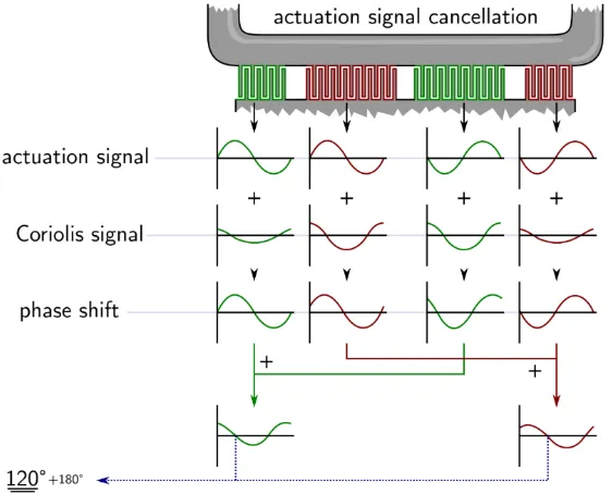
[image:12.595.148.429.185.412.2]

A mathematical model for the voltage cancellation will be derived in this section. Figure 2.5 shows how the capacitive readouts of the combs are summed to produce two output signals.

Figure 2.5: Novel capacitive readout of the Coriolis mass flow sensor. Figure taken from [3].

The actuation mode signalSacan be described by

Sa =Aa·sin(wt) (2.3)

whereAais the amplitude of actuation mode signal andωis the angular frequency of the actuation mode vibration. Similarly, the Coriolis mode signalSccan be described by

Sc=Ac·cos(wt) (2.4)

whereAcis the amplitude of Coriolis mode signal. The two output signalsS1 andS2 are sums of Coriolis mode signals and actuation mode signals. They can thus be described using the following equations:

S1 =Acs·cos(ωt) +Aas·sin(ωt) +Acl·cos(ωt)−Aal·sin(ωt)

= [Aas−Aal]·sin(ωt) + [Acs +Acl]·cos(ωt) (2.5)

S2 =Acs·cos(ωt)−Aas·sin(ωt) +Acl·cos(ωt) +Aal·sin(ωt)

(13)

2.3. MATHEMATICALMODEL OFCANCELLATION 7

The addition of the subscript s and l indicate the amplitude of the small and large

comb respectively.

The equation forS1 can be expressed as

[Aas−Aal]·sin(ωt) + [Acs+Acl]·cos(ωt) = Asum·sin(ωt+ϕ1) (2.7)

for some value of Asum andϕ1 where Asum is the amplitude of the combined signal andϕ1 is the phase. This equation can be rewritten to

sin(ωt) + Acs+Acl

Aas−Aal

·cos(ωt) = Asum

Aas−Aal

·sin(ωt+ϕ1) (2.8)

To find an equation for the phase, the trigonometric identity

cos(ϕ)·sin(ωt) + sin(ϕ)·cos(ωt) = sin(ωt+ϕ) (2.9)

can be rewritten to

sin(ωt) + tan(ϕ)·cos(ωt) = 1

cos(ϕ) ·sin(ωt+ϕ) (2.10)

From equation 2.7 and 2.8, it follows that

tan(ϕ1) =

Acs+Acl

Aas−Aal

⇒ϕ1 = arctan(

Acs+Acl

Aas−Aal

) (2.11)

Following the same derivation forS2 results in a similar expression for the phase

tan(ϕ2) =

Acs+Acl

Aal−Aas

⇒ϕ2 = arctan(

Acs+Acl

Aal−Aas

) (2.12)

The phase difference betweenS1 andS2 is thus given by

ϕ =ϕ2−ϕ1 = arctan(

Acs+Acl

Aal−Aas

)−arctan(Acs+Acl

Aas−Aal

) (2.13)

For small angles, the approximation arctan(x) ≈ x can be used and the phase

dif-ference can be simplified to:

ϕ≈2·(Acs+Acl

Aal−Aas

) (2.14)

Now that an equation for the phase difference between the two output signals has been derived, the next step is to rewrite the equation to show how the phase shift depends on the amount of cancellation. The cancellation is controlled by the high-frequency carrier signals connected to the capacitive combs. The two large combs are multiplied by a carrier signal with an amplitudeAcarl while the small combs are multiplied by a carrier signal with an amplitude Acars. The transfer function of the

(14)

the actuation mode signal components and the Coriolis mode signal components will also be proportional to the amplitude of the carrier signal. Adjusting the amplitude of the carrier signal will change the amount of cancellation.

It is known that the actuation mode signal is proportional to the number of finger pairs in the comb. For the large comb, this is Nl. It is also known that the amplitude

of the actuation mode signal is proportional to the distance of the comb from the center of the sensor. The finger pairs are evenly spaced so the distance is directly proportional to the number of finger pairs as well. The distance between the midpoint of the large comb and the center of the sensor is thus Nl

2 . As stated before, the amplitude of the actuation mode signal is also proportional to the amplitude of the carrier signal. Thus, the amplitude of the actuation mode signal of the large comb

Aal can be described by:

Aal∝Nl·

Nl

2 ·Acarl (2.15)

A similar derivation follows for the small comb with Ns finger pairs. The small comb is directly adjacent to the large combs, so its distance from the center of the sensor is given by Ns

2 +Nl.

Aas ∝Ns·(

Ns

2 +Nl)·Acars (2.16)

Equation 2.15 and 2.16 can be combined to find an expression for Aas in terms of

Aal:

Aas

Aal

= Ns·(

Ns

2 +Nl)

Nl· N₂l

·Acars

Acarl

⇒Aas=

Ns·(N₂s +Nl)

Nl· N₂l

·Acars

Acarl

·Aal (2.17)

A similar relationship can be derived for the Coriolis mode signals. The Coriolis mode signals are only proportional to the number of finger pairs in the comb and the amplitude of the carrier signal:

Acl ∝Nl·Acarl (2.18)

Acs ∝Ns·Acars (2.19)

Dividing these equations yields:

Acs

Acl

= Ns

Nl

· Acars

Acarl

⇒Acs =

Ns

Nl

· Acars

Acarl

·Acl (2.20)

(15)

2.3. MATHEMATICALMODEL OFCANCELLATION 9

for the phase difference 2.13. After some algebraic manipulation, the equation can be reduced to:

ϕ ≈2Acl

Aal

·G (2.21)

whereGis given by:

G= Acarl+

Ns

Nl ·Acars

Acarl−(2N_Ns

l + (

Ns

Nl)

2₎_·_A cars

(2.22)

This equation is interesting because the ratio of the amplitude of the actuation mode signal Al and the Coriolis mode signal Ac are constant at a given flow rate. This means that the amount of phase shift is controlled by the value of the gain G. The

[image:15.595.161.454.362.599.2]

number of finger pairs are physical properties of the sensor which means the value of the gain is dependent only on the amplitude of the carrier signals. In fact, the gain is actually dependent only on the ratio between the large and small carrier signals.

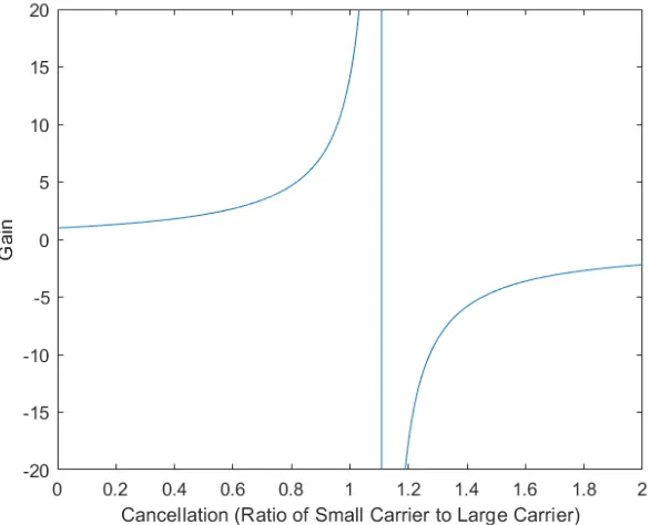
Figure 2.6: Change in sensitivity due to cancellation of actuation mode signal.

The large combs of the sensor used in this experiment contain 29 finger pairs, and the small combs contain 11 finger pairs. A plot of the gain for different values of the cancellation is shown Figure 2.6 (MATLAB code included in Appendix A.1). The cancellation is defined as the ratio between the small carrier signal and the large carrier signal i.e. Acars

Acarl. When the value of the small carrier signal is zero, the value

of G is 1. This is expected, since this corresponds to zero cancellation so there

(16)

leads an increase in the value of G. This means that at the same flow rate, there

(17)

Chapter 3

Measurement Setup

Measurements of the phase shift will be carried out to investigate the effect of the cancellation on the sensitivity of the Coriolis mass flow sensor. As described previ-ously, the change in sensitivity (i.e. the gain) is controlled by the ratio between the small and large carrier signals. During the measurements, the carrier signal in the large combs will be kept constant and the carrier signal in the small combs will be varied to control the cancellation.

Amplitude measurements of the output signals without mass flow will first be performed at various small comb carrier voltages to verify that the sensor outputs are functioning properly and that the actuation mode signal is being cancelled. Af-terwards, the phase shift between the output signals will be measured for varying mass flows and voltages.

Before measurements can be taken with the Coriolis mass flow sensor, a vi-brometer measurement needs to be performed to find the resonance frequency of the sensor. The reason for doing so is detailed in the next section, and the remainder of this chapter discusses the measurement setup and process.

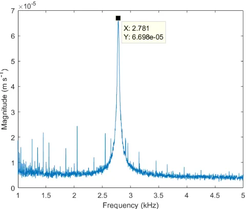
3.1 Vibrometer Measurement

To determine the resonance frequency of the sensor, a laser Doppler vibrometer (Polytec OFV-552 Fiber Vibrometer) is used to measure the magnitude of the vibra-tion velocity at different frequencies. This is done to find the optimal frequency for the actuation current. The actuation current should not be confused with the actu-ation mode signal: the actuactu-ation current is the input current that causes the sensor to vibrate in the twist mode, whereas the actuation mode signal is the component of the output from the capacitive comb that is caused by the twist mode vibration.

A laser Doppler vibrometer uses a laser to measure the vibration velocity of an object. When a wave is reflected by a moving object, there will be a shift in the

(18)

[image:18.595.162.403.92.296.2]

Figure 3.1: The magnitude of the vibration for different frequencies.

frequency of the wave related to the velocity of the object. The wave in this case is the beam of light from the laser, and it is used to determine the vibration velocity [8]. The vibrometer measurement for frequencies from 1 kHz to 5 kHz is shown in Figure 3.1 (MATLAB code included in Appendix A.2). There is a clear peak at the resonance frequency of the sensor, which occurs at 2.78 kHz. This will be used as the frequency of the actuation current.

3.2 Sensor and Electrical Components

The Coriolis sensor chip (mask design in Appendix B.1) is glued to a small modular PCB, and wire bonds are used to make connections between the chip and the PCB. This PCB can then be interfaced with a chip holder board [7]. The chip holder board provides many electrical connections that allow inputs and outputs to be connected to the chip easily using coaxial cables, as shown in Figure 3.2.

(19)

[image:19.595.93.536.85.237.2]

3.3. FLUIDICSETUP 13

Figure 3.2: Image of the front and back of the chip holder board.

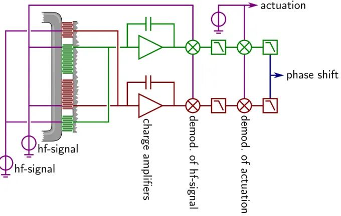
Figure 3.3: Schematic of electronic measurement setup. Figure adapted from [3].

A diagram of the electronic measurement setup is shown in Figure 3.3. The outputs of the large and small comb pairs are cross connected. These outputs are then connected to a charge amplifier to transform the capacitance to a voltage. Next, the signals are demodulated to remove the high-frequency carrier signal. Finally, the signals are connected to two more SR830 lock-in amplifiers to determine the phase shift. Both the charge amplifier and demodulation electronics are in-house developed boards.

3.3 Fluidic Setup

[image:19.595.145.485.280.496.2]

(20)

sup-ply is connected to the chip holder board, and the gas flows through the chip. On the other side, the flow controller (Bronkhorst EL-FLOW Select F-201CV) is connected to adjust the flow rate of the nitrogen passing through the chip. The maximum volu-metric flow rate of the flow controller is 20 mln/min. For nitrogen pressurized at 6 bar at room temperature (20 ◦_{C), this corresponds to a mass flow of 8.299 grams per}

[image:20.595.112.455.216.359.2]

hour. The flow rate can be set using the FlowPlot (V3.34) software as a percentage of the maximum flow rate.

Figure 3.4: Illustration of fluidic measurement setup. Figure adapted from [9].

3.4 Measurement Process

(21)

Chapter 4

Measurement Results

4.1 Amplitude Measurements Without Mass Flow

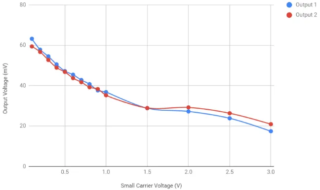
[image:21.595.151.475.517.710.2]

Some initial measurements are taken without mass flow to verify that the sensor is functioning properly. The carrier signals are 5 MHz square waves, and the actuation current was chosen as a 2.807 kHz sine wave. Initially the measured resonance frequency was used for the actuation frequency (2.78 kHz), but it was tuned slightly to find a value that produced the best results. The sync channel of the function generator is used as the large carrier signal and has a constant peak-to-peak voltage of 4 V. The small carrier signal is the standard output of the oscilloscope and the voltage is varied manually. Since there is no flow, the phase shift is not of interest and the amplitude of the sensor’s output signals is measured. The results of the measurement have been plotted in Figure 4.1 (raw data included in Appendix C.1).

Figure 4.1: Sensor output voltage for increasing cancellation. All voltages are peak-to-peak.

(22)

The small carrier voltage controls the amount of cancellation, and as the voltage of the small carrier is increased, so does the cancellation. Since the actuation mode signal is being cancelled, the sensor’s output decreases in amplitude as expected. The amplitude of both outputs remain close to each other, so the cancellation seems to be quite even for both sets of comb pairs. Since the sensor seems to be working fine, the next step is to measure the phase for different mass flows and cancellations.

4.2 Phase Measurements With Mass Flow

The phase measurements use the same carrier signal and actuation current as de-scribed in the previous section (5 MHz square wave carrier and 2.807 kHz sine actuation current). The small carrier signal is varied from 2 V to 10 V in steps of 1 V. For each value of the small carrier signal, a set of phase measurements for different mass flows is taken.

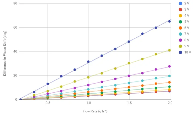
[image:22.595.120.447.516.708.2]

The mass flow controller software specifies steps as percentages of the maxi-mum flow rate of the controller (20 mln/min). The mass flow is varied from 2% to 24% in steps of 2%. For nitrogen gas at 6 bar and room temperature, this corre-sponds to a range of approximately 0.166 g/h to 1.992 g/h. At each flow rate, the phase of the two outputs is recorded. The change in the phase difference between the outputs is then calculated for each flow rate. This change is taken relative to the phase difference between the outputs of the first flow rate (2%). These measure-ments are repeated for each value of the small carrier signal. The results of this measurement is shown in Figure 4.2 (raw data included in Appendix C.2).

(23)

[image:23.595.153.475.95.288.2]

4.2. PHASEMEASUREMENTS WITHMASS FLOW 17

Figure 4.3: Sensitivity of the sensor at different cancellation ratios (defined as the ratio of the small carrier voltage to the large carrier voltage).

At each of the small carrier voltages, the phase shift appears to be linearly pro-portional to the flow rate. For higher carrier voltages, the phase differences are also larger, indicating an increased in sensitivity. Both of these properties are in accordance with the theory.

The sensitivity can be defined as the change in phase shift with respect to the change in mass flow, i.e. the gradient of the line. For each set of measurements, this is calculated using linear regression and the results are included in Appendix C.3. The R-squared coefficient has also been calculated; it is noteworthy that for all measurements, the R-squared coefficient was in excess of 0.998, indicating a very strong linear trend.

The mathematical model derived in section 2.3 defines a relationship between the gain and the cancellation ratio. The cancellation ratio is defined as the ratio of the small carrier signal to the large carrier signal, so the small carrier signals in these measurements can be converted to a cancellation ratio by dividing by 4 (the peak-to-peak voltage of the large carrier signal). A plot of the calculated sensitivities for each cancellation ratio is shown in Figure 4.3.

(24)

(25)

Chapter 5

Conclusion

The results confirm that the change in the phase shift of the output signals can be used as a measurement of the mass flow. At each of the different cancellation ratios, all of the measurements exhibited a very strong linear correlation between the phase shift and the mass flow. Since the relationship is linear, the gradient of the line serves as a measure of the sensor’s sensitivity. The gradients were calculated through linear regression during which the R-squared correlation coefficient was also calculated. All of the R-squared coefficients were in excess of 0.998, further supporting the strong linear relationship.

The sensitivity derived from the measurements and the gain as defined by the model by the model are proportional since both of them determine how the phase changes with respect to the mass flow. Thus, it is expected that the plot of the modeled gain against the cancellation ratio (Figure 2.6) should be similar to the plot of the measured sensitivity (Figure 4.3). The plot of the sensitivity does indeed have a curve shape similar to the plot of the modeled gain, but there is a rather notable difference in the cancellation ratios. According to the model, the actuation mode signal becomes fully cancelled at a cancellation ratio of about 1.1, at which point the gain (or sensitivity) approaches infinity. However, during the measurements, the sensitivity increased much slower with respect to the cancellation ratio. Only a small increase in sensitivity was observed when the cancellation ratio reached 1.0 and 1.5. The sensitivity continued to increase up until the maximum cancellation ratio measurement of 2.5.

The increase in the sensitivity of the sensor as the amount of cancellation is increased supports the theory that cross connecting the capacitive combs allows for the actuation mode signal to be cancelled and larger phase shifts to be observed at the same flow rates. However, the rate at which the sensitivity increases with respect to the cancellation ratio is quite different from the mathematical model.

(26)

(27)

Chapter 6

Discussion and Recommendations

A linear relationship between the mass flow and the phase shift of the sensor outputs was observed. As the amount of cancellation was increased, so did the rate at which the phase shift increased relative to the mass flow (i.e. the sensitivity), supporting the theory. However, the change in sensitivity with respect to the cancellation ratio did not correspond to the change predicted by the mathematical model; the increase in sensitivity was much more gradual. The inaccuracy of the model is likely due to some of the idealized assumptions made in the model, such as neglecting the separation distance between the combs and assuming the capacitive readouts to have perfectly linear properties. A more accurate model should be derived for future research.

One issue encountered was the stability of the sensor. The sensor did not appear to be very stable at times, and different results would be obtained when measure-ments were performed again on a different day or when the sensor was reattached to the chip holder board. Additionally, some noise was observed in the output signals, which became more apparent as the cancellation was increased since the signals become smaller.

Some problems were also encountered with the FlowPlot software for controlling the flow rate. It was possible to measure the flow rate and set target flow rates in the software, but for some reason the flow controller did not respond to the setpoints. Thus, a valve was manually adjusted to reach the target flow rates and the FlowPlot software was only used to measure the current flow rate. If this issue is resolved, the measurement process will become much faster.

The measurement of the phase difference of the sensor outputs can also be im-proved. The measured phase displayed on the lock-in amplifier was not completely stable, so it was be observed for a short period of time and a middle value was recorded. While this did not appear to have a significant impact on the results, it can be improved by increasing the integration time of the lock-in amplifier to provide more stable and accurate results.

(28)

(29)

Bibliography

[1] Bronkhorst High-Tech B.V., “Miniaturization to the extreme: Micro-coriolis mass flow sensor,” 2018, last accessed 25 June 2018. [Online]. Available: https://www.bronkhorst.com/blog/ miniaturization-to-the-extreme-micro-coriolis-mass-flow-sensor/

[2] OMEGA Engineering, “Thermal mass flow working principle, theory and design,” 2018, last accessed 25 June 2018. [Online]. Available: https://www.omega.com/ technical-learning/thermal-mass-flow-working-principle-theory-and-design.html

[3] D. Alveringh, J. Groenesteijn, R.J. Wiegerink, and J.C. Lotters, “A novel capac-itive detection principle for coriolis mass flow sensors enabling range/sensitivity tuning,” Sep. 2015.

[4] Encyclopaedia Britannica, “Coriolis force,” 2018, last accessed 11 June 2018. [Online]. Available: https://www.britannica.com/science/Coriolis-force

[5] T. Schut, “Sensing of multiple parameters in a micro-fabricated flow system,” 2017.

[6] J. Haneveld, T.S.J. Lammerink, M.J. de Boer, and R.J. Wiegerink, “Micro cori-olis mass flow sensor with integrated capacitive readout,” in 2009 IEEE 22nd

International Conference on Micro Electro Mechanical Systems, Jan 2009, pp.

463–466.

[7] D. Alveringh, “Integrated throughflow mechanical microfluidic sensors,” Ph.D. dissertation, University of Twente, 2018.

[8] Polytec GmbH, “Laser doppler vibrometry,” 2018, last accessed 14 June 2018. [Online]. Available: https://www.polytec.com/us/vibrometry/technology/

[9] D. Alveringh, T. Schut, R. Wiegerink, W. Sparreboom, and J. Lotters, “Resis-tive pressure sensors integrated with a coriolis mass flow sensor,” in 2017 19th International Conference on Solid-State Sensors, Actuators and Microsystems

(TRANSDUCERS), June 2017, pp. 1167–1170.

(30)

(31)

Appendix A

MATLAB Scripts

A.1 Gain Calculation

1 N s = 11; %Small comb finger pairs

2 N l = 29; %Large comb finger pairs

3 r = N s/N l;

4 A carl = 1; %Large carrier

5 A cars = linspace(0,2,2000); %Vary small carrier (i.e. cancellation ratio) from 0 to 2

6 gain = (A carl + r∗A cars) ./ (A carl - (2∗r + rˆ2)∗A cars); %Calculate gain

7 plot(A cars,gain);

8

9 %Axis limits and labels

10 xlim([0 2]);

11 ylim([-20 20]);

12 xlabel("Cancellation (Ratio of Small Carrier to Large Carrier)");

13 ylabel("Gain");

A.2 Vibrometer Measurement

1 values = Scan.Variables; %Read values from imported table

2 values(:,1) = values(:,1)/1000; %Convert frequency to kHz

3 plot(values(:,1),values(:,2));

4

5 %Axis labels

6 xlabel("Frequency (kHz)")

7 ylabel("Magnitude (m sˆ{-1})")

(32)

(33)

Appendix B

Coriolis Mass Flow Sensor

[image:33.595.174.454.334.471.2]

B.1 Mask Design

Figure B.1: Mask design of the Coriolis mass flow sensor. Design created in Clewin by R.J. Wiegerink.

(34)

(35)

Appendix C

Measurement Data

[image:35.595.167.459.356.717.2]

C.1 Amplitude Measurements Without Mass Flow

Table C.1: Output amplitude measurements without mass flow.

Small Carrier (V Peak-to-Peak)

Output 1 (mV Peak-to-Peak)

Output 2 (mV Peak-to-Peak)

0.1 63.2 59.4

0.2 57.8 56.7

0.3 54.5 52.7

0.4 50.5 48.9

0.5 47.2 46.8

0.6 45.4 43.7

0.7 42.8 41.7

0.8 40.7 39.2

0.9 37.6 38.3

1.0 36.8 35.2

1.5 28.8 28.9

2.0 27.2 29.2

2.5 23.8 26.3

3.0 17.4 20.9

(36)

[image:36.595.123.448.150.465.2]

C.2 Phase Measurements With Mass Flow

Table C.2: Phase measurements for small carrier of 2 V (peak-to-peak).

Mass Flow (Percentage

of Max. Flow Rate) Phase 1 (deg) Phase 2 (deg)

2 -107.14 70.09

4 -101.67 76.16

6 -96.42 82.00

8 -91.41 87.59

10 -86.60 93.02

12 -82.22 98.10

14 -78.19 102.86

16 -74.22 107.43

18 -70.51 111.66

20 -67.05 115.95

22 -63.73 119.91

(37)

[image:37.595.141.492.93.419.2]

C.2. PHASEMEASUREMENTSWITHMASSFLOW 31

2 -106.94 70.85

4 -101.45 77.03

6 -96.18 82.96

8 -91.05 88.56

10 -86.42 93.84

12 -82.05 99.03

14 -77.91 103.87

16 -73.91 108.34

18 -70.30 112.74

20 -66.71 116.80

22 -63.62 120.60

(38)

[image:38.595.111.461.90.420.2]

2 -106.67 71.37

4 -101.36 77.47

6 -96.02 83.41

8 -91.14 89.08

10 -86.39 94.70

12 -82.16 99.76

14 -78.07 104.59

16 -74.23 109.26

18 -70.64 113.37

20 -67.13 117.74

22 -63.98 121.87

(39)

[image:39.595.141.493.92.420.2]

2 -106.53 71.52

4 -101.31 77.81

6 -96.07 83.86

8 -91.18 89.85

10 -86.55 95.36

12 -82.38 100.59

14 -78.38 105.37

16 -74.66 110.16

18 -71.14 114.81

20 -67.83 119.14

22 -64.61 123.18

(40)

[image:40.595.110.464.90.420.2]

2 -106.03 71.80

4 -100.88 78.12

6 -96.15 84.42

8 -91.36 90.38

10 -86.94 95.98

12 -82.71 101.53

14 -78.88 106.56

16 -75.41 111.42

18 -72.06 116.15

20 -68.79 120.77

22 -65.99 125.22

(41)

[image:41.595.140.493.92.420.2]

2 -105.20 72.21

4 -100.36 78.84

6 -95.71 85.25

8 -91.01 91.47

10 -87.02 97.21

12 -83.06 102.93

14 -79.47 108.34

16 -75.91 113.50

18 -72.77 118.49

20 -69.77 123.45

22 -67.08 128.20

(42)

[image:42.595.110.463.90.420.2]

2 -104.03 73.02

4 -99.34 80.13

6 -95.23 86.85

8 -91.10 93.13

10 -87.14 99.57

12 -83.63 105.59

14 -80.42 111.45

16 -77.09 117.23

18 -74.40 122.49

20 -71.45 127.66

22 -69.28 132.94

(43)

[image:43.595.142.494.93.420.2]

2 -101.06 74.70

4 -97.71 81.87

6 -93.92 88.98

8 -90.54 96.11

10 -87.38 103.53

12 -84.24 110.11

14 -81.14 116.55

16 -78.59 123.06

18 -76.47 129.65

20 -74.20 135.41

22 -72.06 141.52

(44)

[image:44.595.105.469.90.420.2]

2 -95.49 77.12

4 -93.02 85.97

6 -90.95 94.82

8 -89.12 103.05

10 -86.58 111.03

12 -85.03 119.21

14 -82.67 126.52

16 -80.41 134.38

18 -79.00 141.88

20 -77.64 149.80

22 -76.15 156.31

(45)

C.3. SENSITIVITY ANDCANCELLATION RATIO 39

[image:45.595.130.499.196.445.2]

C.3 Sensitivity and Cancellation Ratio

Table C.11: Sensitivity (gradient) for each set of phase measurements, calculated using linear regression. The R-Squared coefficient has been calcu-lated, and the small carrier voltage has been converted to a cancella-tion ratio.

Small Carrier (V Peak-to-Peak)

Cancellation Ratio

Sensitivity (deg / (g h-1₎₎

R-Squared Coefficient

2 0.50 3.88 0.999

3 0.75 3.93 0.998

4 1.00 4.67 0.999

5 1.25 5.91 0.999

6 1.50 7.95 0.999

7 1.75 10.71 0.999

8 2.00 15.11 0.999

9 2.25 22.72 1.000