Distributed Symbolic Reachability Analysis

(1)

Distributed Symbolic Reachability

Analysis

Master Thesis

Author:

Graduation Committee:

Wytse Oortwijn (s1247379)

Prof. Dr. J.C. van de Pol

MSc. T. van Dijk

Dr. S.C.C. Blom

Formal Methods and Tools (FMT)

University of Twente

(2)

Abstract

Model checking is an important tool in program verification and software validation. Model checkers generally examine the entire state space of a model to find behaviour that differs from a given formal specification. Most temporal safety properties can be verified via reachability analysis. A major limitation is the state space explosion problem, which occurs when the state space does not fit into the available memory.

State spaces can efficiently be stored as Binary Decision Diagrams (BDDs), a data struc-ture used to efficiently represent sets. The BDD representations of state spaces can then be manipulated via BDD operations, which enablessymbolic reachability analysis. Moreover, more hardware resources can be employed. By increasing processing units and available memory, larger state spaces can be stored and processed in less time.

This thesis focuses on symbolic reachability analysis, in addition to adding hardware re-sources by using a network of workstations. Our research goal is to implement distributed BDD operations that scale efficiently along all processing units and memory connected via a high-performance network.

Compared to existing work on distributed symbolic reachability, we use modern techniques and components, like Infiniband and RDMA, to reduce network latency. Furthermore, we use hierarchical private deque work stealing to implement efficient load-balancing. Finally, we at-tempt to use the idle-times of workers as efficient as possible by overlapping RDMA roundtrips as much as possible.

We designed an RDMA-based distributed hash table and private deque work stealing algo-rithms. Both components are micro-benchmarked in detail and used to implement the actual BDD operations for distributed symbolic reachability. The algorithms are evaluated by perform-ing symbolic reachability over a number of BEEM models.

(3)

Introduction

An important tool in program verification and software validation is model checking. Given a formal specification, model checking algorithms analyse program behaviour by exhaustively searching all reachable program states, which constitute astate space graph. State spaces often grow exponentially with the size of the program model, which may lead to well-known state space explosions. These exponential blow-ups occur when program states do not longer fit into the available memory. State space explosions may arise very quickly in practice, making them a major limitation in modern software verification.

Several attempts have been made to attack state space explosions. Those attempts include reduction techniques like Partial Order Reduction [57] and Bisimulation Minimization [30]. In addition, state spaces can be compressed, so that more states fit into the available memory. Binary Decision Diagrams (BDDs) can be used for such compression, as BDDs can efficiently represent sets. Moreover, state spaces can efficiently be manipulated by manipulating their BDD representatives, which enablessymbolic model checking. BDDs can significantly improve the space complexity of state spaces compared to explicit representations [32], which motivates symbolic model checking. Alternative effective compression techniques include SAT-based approaches [11], inductive verification (e.g. IC3) [20], and other variants on decision diagrams (e.g. MDDs, LDDs, and ZDDs) [26,31,75], but this thesis focusses only on BDDs.

In addition to techniques for reduction and compression, more hardware resources can be employed [34,51,79,80]. By increasing processing units and available memory, larger state spaces can be stored and processed in less time. Therefore, much research has been devoted to parallel algorithms for both symbolic and explicit model checking [41,44,75,79,80]. As a result, good speedups are obtained on many-core clusters. The parallel BDD package Sylvan [75], for example, reaches impressive speedups up to 38 with 48 cores.

Apart from parallel implementations, also distributed symbolic verification algorithms have been proposed [25,26,48,56,58,68] (see Section 5.1 for more detail). Most approaches were motivated by the expensiveness and limitations of hardware scalability of many-core machines. Compared to sequential runs, no speedups were obtained by most implementations, but very large state spaces could be stored due to the large amount of available memory. Speedups remained low, since BDD operations perform only small amounts of computation per memory access. Distributed implementations thus require many remote memory accesses, which easily makes network latency a performance bottleneck.

(6)

the RDMA devices instead, allowing CPUs to continue with other computational tasks. RDMA supports zero-copy data transfers, which means that no memory copies are performed when sending or receiving packets, unlike traditional protocols such as TCP [65]. Furthermore, RDMA also supports kernel bypassing, which avoids communication with the operating system kernel before handling packets. As a result, one-sided RDMA operations can be performed within 3µs on Infiniband hardware [3], compared to 60µs with TCP on Ethernet hardware [24]. The low latencies of RDMA and its CPU efficiency justify a renewed attempt in distributed symbolic verification.

Moreover, at the time of writing, Infiniband hardware is comparable in price to their Eth-ernet counterparts, which makes scaling along high-performance hardware just as expensive as scaling along standard Ethernet hardware. Some recent research, for example the RDMA-based key-value store Pilaf [24] (2014), was motivated by this cheap scalability. In addition, high-performance networks support an almost unlimited number of processing units and memory, in contrast to individual multi-core machines. Combining these reasons with the cheap scalability and low latencies of modern networking hardware motivates our research, and may allow more efficient distributed model checking.

1.1 Research Goals

In this thesis we present distributed algorithms for reachability analysis, based on BDDs. The al-gorithms are specialized for high-performance networks, like Infiniband, by making use of RDMA. To the best of our knowledge, no other attempts have been made to distribute symbolic verifica-tion with an RDMA-based approach. By experimental evaluaverifica-tion and reflecverifica-tion on the proposed algorithms, we answer the following main research question:

Research question (RQ): How efficient can RDMA-based distributed implementa-tions of BDD operaimplementa-tions scale along all processing units and available memory connected via a high-performance network?

To determine how RDMA can most efficiently be used by BDD operations, we focused on three important design considerations, given in [32], for efficient distributed symbolic state-space generation. These considerations are: data distribution, load-balancing maintenance, and re-duction of communication overhead and latency. Also exploiting data-locality is an important consideration, as part of data distribution [26]. To answer the main research question, we focused on all four considerations, resulting in several subquestions:

Subquestion 1 (SQ1): How can the storage and retrieval of data efficiently be man-aged to minimize their latencies?

Subquestion 2 (SQ2): How can the total computational work be divided and dis-tributed to maximize scalability along processors over a high-performance network?

Subquestion 3 (SQ3): How can the idle-times of processes be minimized while per-forming network communication?

(7)

1.2 Methods and Contributions

This section discusses the research methods used to answer the subquestions. In addition, our contributions and findings are given.

1.2.1 Data Distribution

To answerSQ1, we investigated existing high-performance distributed storage techniques, includ-ing hash tables and key-value stores. Existinclud-ing work includes Pilaf [24], Nessie [67], HERD [10], and FaRM [5], which all use RDMA to reduce latency. With the exception of HERD, all these im-plementations either use Cuckoo hashing [52] or Hopscotch hashing [46] to resolve hash collisions. HERD only uses one-sided writes to minimize the required number of roundtrips, at the cost of CPU-efficiency, which we would like to retain. Cuckoo hashing usesk≥2 hash functions, which means k roundtrips when accessing remote buckets. Hopscotch hashing uses neighbourhoods, which can be retrieved with a single roundtrip, making Hopscotch arguably more efficient than Cuckoo. However, both hashing schemes require expensive relocation procedures when data can not be inserted. Those procedures may require many extra roundtrips and expensive distributed locking mechanisms. We argue that linear probing is more efficient, since it does not use such relocation procedures.

In Chapter3 we present an RDMA-based distributed hash table that uses linear probing to reduce the number of roundtrips and thus reduces latency. The hash table supports one operation, namelyfind-or-put, that either adds data or gives a positive result. To minimize waiting-times, find-or-put overlaps roundtrips as much as possible, which further reduces latency. Because linear probing examines buckets that are consecutive in memory, a range of buckets, which we call chunks, can be obtained with a single roundtrip. By increasing chunk sizes, higher load-factors are supported and require fewer roundtrips, at the cost of slightly higher latencies.

A peak-throughput of 3.6×106 _{op/s is reached on an Infiniband network with 10 machines.}

On average, find-or-put finds intended buckets within 9.3µs with a load-factor of 0.9 when targeting remote memory. On the other hand, by adding processes, the throughput of the RDMA devices get saturated, which significantly affects the scalability of processes when also scaling along machines. Solving this limitation would require improving data-locality, as well as reducing the required number of roundtrips.

1.2.2 Load-Balancing Maintenance

Graph algorithms can effectively be parallelized by usingfine-grained task parallelism [8], which includes operations on BDDs. Due to the success of the parallel symbolic BDD package Syl-van [75] by applying dynamic load-balancing via work stealing, we investigated hierarchical work-stealing approaches to answer SQ2. Existing approaches include Scioto [35] and Hot-SLAW [62], which both use split deques for storing tasks. Both approaches require expensive locking mechanisms when performing steals. Instead, we focus on private deque work stealing, similar to [50], due to the absence of locking and the decrease in roundtrips compared to split deques.

Min et al. [62] propose hierarchical victim selection to exploit locality, thereby reducing the average number of roundtrips. Also hierarchical chunk selection is proposed to adjust the number of tasks to steal, based on communication costs. Another technique that may increase performance is leapfrogging [77], that allows victims to steal back from their thiefs, thereby helping thiefs to complete parts of their original work.

(8)

the ideas of [50], but requires fewer roundtrips and supports hierarchical victim selection and leapfrogging. Due to time constraints, we were not able to also implement hierarchical chunk selection. Relative to HotSLAW, speedups up to 34.3 are reached for local steals and 9.3 for remote steals. On the other hand, HotSLAW generates less overhead when executing tasks. This is because HotSLAW supports tasks with variable-sized inputs and outputs, whereas our implementation does not. We solved this by using extra shared data structures, which are slightly less efficient than HotSLAW. Our implementation can likewise be optimized, but due to time constraints we were not able to do so. Implementing hierarchical chunk selection and reducing overhead would allow hierarchical work-stealing that ismore efficient than the current state-of-the-art.

1.2.3 Efficient Communication

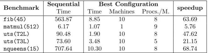
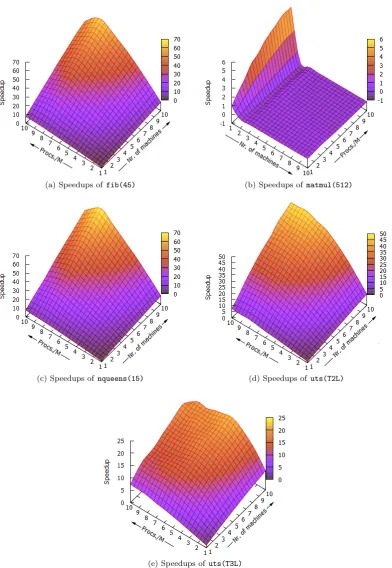
To answerSQ3, we investigated ways to most efficiently use RDMA in the various components of our BDD implementation. To minimize communication overhead we use one-sided RDMA, so that the CPUs on the targeted machines are not invoked. Wherever possible, we employ latency hiding via pre-fetching by overlapping roundtrips as much as possible. In the hash table design, multiple chunks are queried simultaneously, thereby reducing waiting times. Furthermore, hierarchical work stealing is used to exploit locality, reducing the overall idle-times of processes. Chapter 5 presents the designs of our distributed BDD operations. We give asynchronous operations for consulting the shared memoization cache, enabling cache requests to be overlapped with other computational work. The BDD operations are implemented with UPC [27] and evaluated by performing reachability analysis over various BEEM models [53]. Compared to sequential runs, speedups are obtained by using a network of computers. Furthermore, scaling along computers does not decrease performance, and allows more memory to be used. Relative to two computers, each using 8 processes, speedups up to 5.18 are reached by scaling to 10 computers.

We observed that, rather than network latency, the main bottleneck was caused by the limited throughput of RDMA devices. To increase scalability, it iskeyto minimize the number of RDMA operations, as a first priority. We mainly focused on reducing waiting-times and minimizing communication overhead by employing RDMA, but scalability can still be improved. HERD, for example, is a distributed hash table that only uses one-sided RDMA writes as a message passing alternative, thereby achieving a minimal number of roundtrips, at the cost of CPU efficiency. By employing this technique, communication overhead is increased, but fewer RDMA roundtrips are generated, thereby allowing more processes to be used before the RDMA devices get saturated, which in turn increases both scalability and maximal achievable throughput.

1.3 Structure

Chapter 2 provides details on Infiniband network and gives various programming models us-able in combination with RDMA. We chose to use a PGAS abstraction, whose operations are also explained. Chapter 3 presents our distributed hash table design that uses linear probing. Evaluational results of the latency and throughput of find-or-put are also given. Chapter 4

discusses work stealing techniques and present a hierarchical private-deque work stealing design. The implementation is evaluated by running several benchmarks and comparing the results with HotSLAW. Chapter 5 presents the design of our distributed BDD operations. The operations are evaluated by performing reachability analysis on several BEEM models. Finally, Chapter 6

(9)

Chapter 2

Preliminaries on Partitioned

Global Address Space

Programming

2.1 Introduction

In this chapter, the Infiniband network architecture is discussed (Section 2.2). In particular, the Remote Direct Memory Access feature of Infiniband is discussed (Section 2.3), together with various programming models that support RDMA (Section 2.4). In our research, we use the Partitioned Global Address Space programming model, whose operations are discussed in Section 2.5. Finally, the performance of various RDMA operations are determined via micro-benchmarking (Section2.6).

2.2 The Infiniband Architecture

Infiniband [1] is specialized hardware used to construct high-performance networks. Infiniband is manufactured by Microsoft and Mellanox. The specialized hardware includes switches, Network Interface Cards (NICs) [54], and interconnects that support bandwidths up to 300 GB/s. The interconnects use a bidirectional serial bus to keep communication costs low. Experimental evaluation of the algorithms proposed in this thesis are performed on a network of 10 machines, connected via a 20 GB/s Infiniband network.

At the time of writing, the prices of Infiniband hardware are comparable to their Ethernet counterparts [24]. As an effect, scaling along high-performance hardware is just as expensive as scaling along traditional Ethernet hardware. This motivated some recent research in the use of RDMA in non-performance computing [24].

(10)

Operation UD UC RC RD

Send/Receive X X X X

RDMA write X X

RDMA read X

Atomic operations X

Table 2.1: The different operations supported by the various service types used by Infiniband.

As an example, suppose that two nodes A andB need to communicate over an Infiniband network. Both nodes create a Queuing Pair, which they connect, so that messages placed in the Send Queue ofAare transmitted to the Receive Queue ofB, and vice versa. The Channel Adapters of A and B thus forward messages placed in the Send Queue and process messages placed in the Received Queue. In addition to a Queuing Pair, aCompletion Queue can be used. After having processed a message from the Receive Queue, it can be pushed to the Completion Queue, thereby allowing the CPUs to check the status of messages.

2.3 Remote Direct Memory Access

One of the features supported by Infiniband networks isRemote Direct Memory Access (RDMA), which allows nodes to directly access the memory of other nodes, without necessarily invoking their CPUs. RDMA operations are handled by the Channel Adapters instead, which are able to access the main-memory of their host machine via the PCI-E bus. Using RDMA further reduces network latency, since RDMA supportszero-copy data transfers and kernel bypassing.

Traditional protocols, like TCP, require multiple memcopies when transferring data [65]. To illustrate, TCP packets are first copied from application memory to kernel memory, then send over the network, and finally copied from kernel memory to the application memory of the node that received the packet. As an effect, several context switches are performed. In RDMA, the network stack is completelybypassed, as messages are directly pushed on a Send Queue on the Channel Adapter. Furthermore, the Queuing Pairs reside in the memory of the Channel Adapters themselves, which prevents memcopies. As a result, RDMA operations can be performed within 3µson Infiniband hardware [3], compared to 60µswith TCP on Ethernet hardware [24].

Sharing Memory. To support RDMA operations on remote memory, the Channel Adapters need to be aware of the blocks of memory exposed via RDMA. Therefore, a blocks of memory can be registered at the Channel Adapters as beingshared. In Infiniband terminology, a consecutive block of shared memory is called a Memory Region. Every memory region can be accessed via local and remote addresses. For every Memory Region, the Channel Adapters hold a lookup table, so that remote addresses can be translated to local addresses. Prior to using RDMA, the remote addresses of the Memory Regions can be transmitted via MPI. In addition, permissions to RDMA-exposed memory can be specified via so-calledProtection Domains.

(11)

t1 t2 . . . tn

(a) Shared Memory

t1 t2 . . .

. . . tn

(b) Distributed Memory

Figure 2.1: Herenthreadst1, . . . , tnare displayed in ashared memoryand adistributed memory

setting. Dashed edges represent communication links between threads.

a connection between two nodes in which data is not guaranteed to arrive, because Ack and Nak packets are not used. Compared to RC, less network traffic is generated, thereby allowing higher throughputs. In theUnreliable Datagram (UD) service type, no responses are expected, similar to traditional UDP. Therefore, RDMA is not supported. However, Grant et al. [61] pro-pose support for RDMA over connectionless protocols, including UD, to improve performance even further. Finally, theReliable Datagram (RD) service type can be used, which is similar to UD, but a reliable connection is guaranteed, since Ack and Nak packets are used upon message retrieval.

In our research, we use RC, since it allows a reliable connection, and therefore contributes to the correctness of the algorithms. However, some operations might be performed under unreliable service types, thereby increasing throughput. As future work, it would for example be interesting to use UD, together with [61], to further increase performance.

2.3.1 RDMA Operations

Infiniband supports various types of operations. Firstly, standard message passing is supported viasend andreceiveoperations. Thesend operation puts a message on the Receive Queue of the targeted node andreceivepolls the Receive Queue for incoming messages.

One-sided RDMA operations only use Send Queues and ignore Receive Queues. When a Channel Adapter receives a one-sided RDMA message, it directly executes its operation on the given location in main-memory. By not using the Received Queue, the CPUs of the targeted nodes are never invoked and are not aware of the one-sided operations executed by the Channel Adapters. One-sidedwriteoperations do not generate a response. One-sidedreadoperations, on the other hand, require the targeted node to give a response, which is written to the Completion Queue of the node that initiated the operation.

Two-sided RDMA operations also use the Receive Queue, in addition to the Send Queues. The CPUs of the targeted nodes need to pop messages from the Receive Queue to process them. Two-sided operations can, for example, be used to support memory operations that are too complex for one-sided operations. Although the CPUs of both machines are involved, performance is still high, since the network stack is still bypassed and zero-copy data transfers are still used.

(12)

t1 t2 . . .

. . . tn

(a) PGAS

t1 t2 . . .

. . . tn

(b) Hybrid PGAS+MPI

Figure 2.2: Herenthreadst1, . . . , tn are displayed in aPGAS setting. Every thread can access

the entire combined memory, of which only a small portion might be local. The global address spaces are represented by dashed rectangles and the local address spaces by solid rectangles.

2.4 Parallel Programming Models

Several parallel programming models exist that expose memory in various ways. Figure 2.1

schematically shows the shared memory and distributed memory models.

Shared Memory. In a Shared Memory Architecture (Figure 2.1a), all threads share a single address space. Communication between threads is done implicitly, as threads may read changes made to the shared memory. This model simplifies programming, as the entire available memory is accessible via a shared address space. On the other hand, data locality is not taken into account, since threads are generally not aware where data resides.

An example of a shared memory architecture is Non-Uniform Memory Access (NUMA), a model often used in computer systems having multiple CPUs. Every CPU has a local memory and is able to access the memories that are local to other CPUs via a shared address space. Different parts of the address space might use different buses, which causes non-uniform accesses.

Another example is the Symmetric Multiprocessing (SMP) architecture, in which all CPUs access memory via the same shared memory bus. This causes memory-intensive applications to generally perform better on NUMA architectures, as the shared bus can become a performance bottleneck.

Distributed Memory. In aDistributed Memory Architecture (Figure2.1b) every thread has a local memory and threads arenot able to access the memory local to another thread. Instead, threads have to performmessage passing, represented by the dashed edges in Figure 2.1b. Dis-tributed memory architectures are often used to create disDis-tributed applications, i.e. programs that run on a network or cluster of computers. Message passing is then performed over the network. A popular interface for message passing is theMessage Passing Interface (MPI) [78]. An advantage of distributed memory is that data locality is fully exploited, since processes only access local memory. Also, programs written with MPI can easily be used on a scalable network of machines.

(13)

Thread 0 Thread 1 . . . Threadn−1

Shared

Private . . .

. . . S[0]

. . .

S[k−1] S[k]

. . .

S[2k−1] S[(n−1)k]

. . .

S[nk−1]

Figure 2.3: The memory layout of a PGAS setting, with ashared arrayS[0], . . . ,S[nk−1], with nthe number of threads andk the number of entries per thread.

data locality.

The PGAS model can be combined with MPI (Figure 2.2b), allowing them to perform mes-sage passing in addition to accessing the global address space. Similar to distributed memory architectures, the PGAS model allows easy scalability along a network of computers.

If PGAS is used in a distributed environment, it can be combined with RDMA, so that remote memory accesses are performed via one-sided RDMA operations. All local memories are then registered as Memory Regions at the Channel Adapters, so that the local memories receive remote addresses. These are used to constitute a global shared address space, making PGAS a high-performance parallel and distributed programming platform.

2.5 PGAS Implementations

Various PGAS implementations exist, including Unified Berkeley C (UPC) [27], Co-array Fortran (CAF) [49], Titanium [6], X10 [55], Chapel [19], and Open Shared Memory (OpenSHMEM) [14]. The languages UPC, CAF, and Titanium are extensions to C, Fortran, and Java, respectively. Chapel and X10 are both programming languages on themselves, which provide direct support for PGAS, task management, and dynamic task load-balancing. A disadvantage is that their structures differ from C, so all existing BDD operations written in C have to be rewritten entirely when using one of these languages. Also interoperability with existing tools, like LTSmin [64], could be problematic.

In our research, we chose to use Berkeley UPC, since it extends on C and supports asyn-chronous memory operations, where OpenSHMEM does not.

2.5.1 Memory Layout

Figure2.3shows the memory layout of a PGAS setting. Suppose thatnthreads are participating. Then every thread can have a portion of shared memory, i.e. memory registered as a Memory Region at the Channel Adapter. We denote all other memory asprivate. Threads thus only have access to their private memory and memory that is shared by other threads.

(14)

Thread 0 Thread 1

Shared

Private . . . .

(a) Schematic view ofmemget

Thread 0 Thread 1

Shared

Private . . . .

(b) Schematic view ofmemput

Figure 2.4: Schematic overview of thememget and memputoperations. In both cases, thread 0 accesses two shared elements owned by thread 1.

2.5.2 Memory Operations

We now discuss a number of operations supported by most PGAS implementations, starting with memgetandmemput. Figure 2.4gives a schematic overview of these two operation. Thememget operation transfers a block of shared memory into an equally-sized block of private memory (Figure 2.4a). Similarly, the memput operation transfers a block of private memory into an equally-sized block of shared memory (Figure 2.4b). Both operations are blocking operations, thereby preventing further execution of the thread until the operation (i.e. the roundtrip over the Infiniband network) has been completed.

Most PGAS implementations provideasynchronousversions ofmemgetandmemput, which we denote bymemget-asyncandmemput-async. Both functions return ahandle, which can be used to synchronize on the roundtrip. Synchronization is performed with the sync operation, that takes a handle as parameter and blocks further execution of the thread until the corresponding asynchronous operation has been completed. Every asynchronous memory operation must be matched by async, otherwise handle leaks may occur, as the maximum number of handles that can be simultaneously opened is 65.536.

Finally, several atomic operations are supported, including cas and fetch-and-add. The cas(b, c, v) operation compares the content of a shared memory location b with a condition c. Only if the content of b matches c, the value v is written to b. After that, the former value of b is returned. The fetch-and-add(b, v) operations reads a shared memory location b and atomically addsvto its content. Theformercontent ofbis returned. Similar tofetch-and-add, most other bitwise operations are also supported, including fetch-and-and, fetch-and-or, fetch-and-xor, etcetera.

2.5.3 Challenges when using UPC

(15)

We also encountered problems when allocating large blocks of memory. It appears that, by default, Berkeley UPC does not support block sizes of more than 220 _{bytes. By default, 64-bit}

integers are used to represent shared pointers, where 10 bits are used to denote the process ID and 20 bits to denote a block. Since buckets are 23bytes in size, only 2₂203 = 220−3= 2

17_bucket

can be stored per process, which is by far not enough for a proper distributed hash table. This can be solved by configuring Berkeley UPC with the--enable-sptr-structflag, that changes the pointer structure to a struct, which supports block sizes up to 232₋_{1 bytes.}

2.6 Performance of One-Sided RDMA

To determine the expected performance of network communication with one-sided RDMA, we measured its latency and throughput by using the OSU Micro-benchmark [2]. This benchmark tests the latency and throughput of several RDMA operations via OpenSHMEM, with various message sizes. Figures2.5and2.6show the latencies of one-sidedmemgetandmemputoperations, respectively, and Figure2.7shows the latency ofmemput.

For small messages, i.e. 16 bytes or smaller, the localmemgetoperations are about 76 times as fast as remotememgetoperations. Localmemgetoperations are performed in 50nson average, and remote memgetoperations in 3.87µs. The local memputoperations, on the other hand, are only 6 times as fast as remotememputoperations. This is because thememput does not require a full roundtrip. We observe that the differences in latency gets smaller, both for memget and memput, when the message size increases. Localmemputoperations take 0.44µson average, and remotememputoperations take 2.68µswith message sizes up to 16 bytes.

(16)

1B 10B 100B 1KB 0 2 4 Message Size Time ( µs )

1KB 10KB 100KB 1M B

0 500 1,000 Message Size Time ( µs ) Local Remote

Figure 2.5: Latency of one-sidedmemgetoperations performed on both local and remote memory.

1B 10B 100B 1KB

1 2 3 Message Size Time ( µs )

1KB 10KB 100KB 1M B

0 500 1,000 Message Size Time ( µs ) Local Remote

Figure 2.6: Latency of one-sidedmemputoperations performed on both local and remote memory.

1B 10B 100B 1KB 10KB 100KB 1M B

103

104

105

106

107

Message size (log)

Op erations / sec on d Local Remote

(17)

Chapter 3

Designing a Distributed Hash

Table for Shared Memory

In this chapter different hashing schemes are compared and discussed. We argue that linear probing is expected to perform best because it requires less roundtrips than other hashing schemes. An analysis of linear probing is given and its expected performance is determined. After that, the design of find-or-put is given and discussed in detail. A peak-throughput of 3.6 million op/s is reached by find-or-puton an Infiniband cluster.

3.1 Introduction

Hash tables are popular data structures for storing maps and sets, since data can be retrieved and stored with time complexityO(1) [69]. Adistributedhash table is a hash table that is distributed over a number of computers. The advantage is that more memory is available, because the memory of every participating computer can be used. A disadvantage is that the performance of hash table operations might be lower due to the latency of the network and bandwidth limitations. Having a high-performance hash table is, however, essential for an efficient implementation of many distributed algorithms, like graph searching.

Our goal is to implement a distributed hash table using the PGAS programming model. The hash table supports only a single operation, namely find-or-put, that either inserts data when it is not already inserted or indices that the data element has already been added before. Secondly, the hash table must be applicable to any sort of memory-intensive high-performance distributed application that requires a hash table. Distributed graph searching or distributed symbolic reachability are merely examples. If needed,find-or-putcan easily be split into two operations,find and insert. We did not implement adeleteoperation or garbage collection due to time constraints, but the hash table can easily be extended to support tombstones. Furthermore, the hash table should require minimal memory overhead, should be CPU-efficient (i.e. not be based on polling), and the latency of find-or-putshould be minimal.

(18)

as much as possible to minimize the waiting-times for roundtrips.

Previous work includes Pilaf [24], which is a key-value store that uses RDMA. Pilaf uses an optimized version of Cuckoo hashing to reduce the number of roundtrips in a worst case scenario. Lookups are performed by the clients, but inserts and deletes are performed by the server to simplify the synchronization of memory accesses. Nessie [67] is an RDMA-based hash table that also uses Cuckoo hashing. In Nessie,all hash table operations are performed by the clients, which makes its implementation more complex than Pilaf. HERD [10] is a key-value store that only uses one-sided RDMA writes and ignores the CPU bypassing features of RDMA to maximize the throughput. FaRM [5] is a distributed computing platform that exposes the memory of all machines in a cluster as a shared address space. A hash table is built on top of FaRM that uses a variant of Hopscotch hashing.

This chapter is structured as follows. Different hashing strategies are compared in Section3.2. We argue that linear probing required the least number of roundtrips. In Section3.3the expected performance of linear probing in a distributed setting is analysed. Section3.4discusses the design of find-or-put. The experimental evaluation of find-or-put is given in Section3.5. Finally, our conclusions are summarized in Section3.6.

3.2 Preliminaries

It is critical to minimize the number of roundtrips required by find-or-put when accessing remote memory to achieve best performance. This is because hash table throughput is directly limited by the throughput of the RDMA devices. This is also shown in the experimental section. Furthermore, the waiting-times for roundtrips contribute to higher latencies of find-or-put. Minimizing the number of roundtrips reduces waiting-times and thus reduces latency. In this section some notation is given, followed by different techniques for solving hash collisions used in related work. After explaining those techniques, we argue that linear probing requires fewer roundtrips.

3.2.1 Notation

A hash table T =hb0, . . . , bn−1iconsists of a sequence of buckets bi usually implemented as an

array. We denote theload-factor ofT byα=m_n, wheremis the number of elements inserted in T andnis the total number of buckets.

A hash function h: U →R maps data from some universe U ={0,1}w _{to a range of keys}

R={0, . . . , r−1}. We assume that every elementx∈U is a single machine word, so in case of a 64-bit architecture,w= 64 andU contains all binary-encoded 64-bit words.

Hash tables use hash functions to map words x∈U to bucketsbh(x) by lettingr < n. Let

x∈U be a word. Then we write x∈bi if bucketbi containsx, otherwise we write x6∈bi. Let

T be a hash table. We writex∈T if there is some 1≤i≤n−1 for whichx∈bi, otherwise we

writex6∈T.

For somex, y∈U withx6=yit may happen thath(x) =h(y). This is called ahash collision. A hash functionhis called a perfect hash function ifhis injective, meaning thathis perfect if ∀x, y∈U.x6=y =⇒ h(x)6=h(y). A perfect hash function is thus collision-free. In practice, the domainU is unknown and often|U| |R|, so usuallyhis not perfect [7].

A family {hi : U → R}i∈I of hash functions, indexed by some set I, is called universal if

∀x, y∈U. x6=y⇒ P r[hi(x) =hi(y)]≤ _|U1| for everyi∈I. A hash function is calleduniversal

(19)

universal if P r[hi(x) = hi(y)] ≤ _|_U1_| for every x, y ∈ U. Universal hash functions have good

theoretical properties, which are used to give theoretical expectations (in Section3.3).

3.2.2 Hashing Strategies

In the ideal case, only a single roundtrip is ever needed byfind-or-putto either find or insert data. This can, however, only be achieved when hash collisions do not occur. Unfortunately, they are very likely to occur in practice, since|U|is much bigger than|R|when a hash function h:U →R is used.

Our aim is to find a hashing strategy that is both CPU-efficient and requires a minimal num-ber of roundtrips both for finding and inserting data. HERD only needs one roundtrip for every hash table operation, at the cost of CPU efficiency [10]. Only one-sided RDMA write operations are used by HERD to make requests to remote processes. These processes continuously poll memory locations to check for incoming requests. This greatly increases hash table throughput, but also limits HERD to be used in CPU-intensive algorithms. We aim to retain CPU-efficiency to keep the hash table usable in such algorithms.

Chained hashing. With chained hashing, every bucket is implemented as a linked list. Adding a data element x∈ U is performed by adding it to the linked list bh(x). Lookups and deletes

can, however, take Θ(m) time in worst case, when allm data items are inserted into the same bucket. However, it can be shown that both successful and unsuccessful lookups require Θ(1 +α) time on average when a universal hash function is used [69], which is constant (as α≤1). As a consequence, also deletes can be performed with a constant number of operations on average, since it uses lookup. Another consequence is that the number of RDMA operations required to perform remote finds and deletes is also constant. Because universal hash functions are very computational intensive, a more efficient hash function is often used in practice that achieves a suboptimal distribution. As an effect, it often happens that linked lists contain more than one element, thus also require more than one RDMA operation on average. Maintaining linked lists causes memory overhead due to storing pointers. Another disadvantage is that caching perfor-mance is poor due to the lack of data locality. Cache lines cannot effectively be used, because buckets are traversed via pointers.

Cuckoo hashing. Cuckoo hashing[52] is an open address hashing scheme that achieves constant lookup and deletion time and expected constant insertion time. The Cuckoo hashing scheme uses k≥2 independent hashing functionsh1, . . . , hk:U →R withhi6=hj for everyi6=j. With

k-way Cuckoo hashing we refer to Cuckoo hashing withkhash functions. Pilaf uses 3-way Cuckoo hashing [24]. By increasingk, higher load-factors are supported, at the cost of memory accesses or network communication. The Cuckoo hashing scheme maintains the following invariant.

Invariant 1 (Cuckoo Invariant). Suppose that k ≥ 2 independent hash functions h1, . . . , hk :

U →R are used by the Cuckoo hashing scheme. Then for every data item x∈U it holds that either x6∈T or x∈bhi(x) for exactly one 1≤i≤k.

(20)

In both cases, a rehashing scheme must be applied, which not only may require a large number of roundtrips, but also a locking mechanism, which is particularly expensive in a distributed environment. By increasingk, the probability of having to perform a relocation decreases.

Lookups require at most k roundtrips, which can be overlapped to decrease waiting times and thus decrease latency. On the other hand, by increasingk, the number of RDMA operations also increases, which reduces the throughput of the hash table.

Bucketized Cuckoo hashing. A variant on Cuckoo hashing, calledBucketized Cuckoo Hash-ing, enables buckets to contain multiple data elements. Each bucket is subdivided intol slots, and bucketized Cuckoo hashing is then called (k, l)-Cuckoo hashing, where k is the number of hash functions used. The bucketized Cuckoo hashing scheme maintains the invariant that every inserted data element x ∈ T is inserted into exactly one of the l slots, owned by one of the bucketsbh1(x), . . . , bhk(x).

Because every bucket contains multiple slots, it is more likely for a data item to be inserted without needing to relocate items. Furthermore, the number of roundtrips required by the hash-ing operations, as well as the length of relocation chains, is linearly reduced by l. Bucketized Cuckoo hashing performs efficient even whenα > 0.9 according to [15]. The designers of Pilaf pointed out that (2,4)-Cuckoo hashing could be very efficient [24].

Hopscotch hashing. Another hashing scheme with constant lookup time and expected constant insertion time is Hopscotch Hashing [46]. The Hopscotch hashing scheme uses a single hash functionh:U →Rand every bucket is assigned to a fixed-sizedneighbourhood. We denote the size of a neighbourhood by a constantH ≥1. The neighbourhood of bucketbi, which we denote

byN(bi), isbiitself, together with the nextH−1 buckets modulon, soN(bi) =hbi, . . . , bjiwith

j= (i+H−1) modn. Hopscotch maintains the following invariant.

Invariant 2(Hopscotch Invariant). Letx∈U be some data item and letN(bh(x)) =hb1, . . . , bHi.

Then eitherx6∈T or x∈bi for exactly one 1≤i≤H.

Alternatively, for every x∈U it holds that x6∈ T or appears exactly once in N(bh(x)). As

a consequence, alookup(x) operation only needs to examineN(bh(x)) in order to determine if

x∈N(bh(x)). Because neighbourhoods are consecutive blocks of memory, they can be obtained

with a single RDMA roundtrip. Lookups can thus be performed with a single RDMA roundtrip. This is a better result than (Bucketized) Cuckoo hashing, which requires k ≥2 roundtrips. A delete(x) operation simply searches for the bucket b∈N(bh(x)) withx∈band emptiesb with

acasoperation. Assuming that thecassucceeds,deletesrequire only two roundtrips. The insert(x) operation examines the neighbourhoodN(bh(x)) and inserts xinto the first

empty bucket it encounters by performing a cas operation. If cas fails, the operation simply searches for the next empty bucket. If no such bucket exists, the insert operation tries to relocate one of the data items in N(bh(x)) in order to make place for x, while still maintaining

Invariant2. This requires a relocation scheme similar to the one used in Cuckoo hashing. Such a scheme chooses some elementy∈N(bh(x)), reads the neighbourhoodN(bh(y)) ofyand tries to

insertyinto that neighbourhood. If the insert fails, the relocation scheme is recursively applied to relocatey in N(bh(y)), otherwisexcan be swapped for y in N(bh(x)). If the recursion depth

reaches a certain threshold, or if none of the items in the neighbourhood can be relocated, a rehashing scheme must be applied. A relocation scheme is very expensive because it requires many roundtrips and a locking mechanism.

(21)

bucket has been found or some thresholdt≥0 has been reached. Linear probing is very cacheline-efficient, because the examined buckets are consecutive in memory.For the same reason, a range of buckets can be obtained with a single RDMA roundtrip when using linear probing in a distributed environment, which reduces the number of roundtrips.

We expect linear probing to require fewer roundtrips than Hopscotch hashing due to the absence of relocation schemes, which require many roundtrips and a locking mechanism. The Hopscotch hashing scheme enabled lookups to be performed with only a single roundtrip, but that does not effectively apply to afind-or-putoperation. Hopscotch hashing could be more efficient when the hash table is used under a read-intensive workload and when the load-factor is very high. On the other hand, inserting enough items to reach such a high load-factor could already make linear probing more efficient, because it does not need to relocate items. Furthermore, it may happen that relocations cannot be performed, which especially holds under high load-factors. We expect that maintaining Invariant2is too expensive for an efficient implementation of find-or-put.

A variant on linear probing is designed by Laarman et al. [7] in the context of NUMA machines. Here, linear probing is performed in a cache line, which the authors called walking-the-line, followed by double hashing to improve the distribution of data. This scheme obtains very high parallel speedups due to the efficient use of data locality. By walking over cache lines, the number of cache misses is minimized. Van Dijk et al. [75] uses this scheme to implement find-or-putfor multi-core symbolic model checking.

Other open addressing schemes. Quadratic probing is similar to linear probing, only the hash sequence increases quadratically rather than linearly. More specifically, a quadratic hash functionh0 :U ×N →R can be derived from h:U →R by choosing c1, c2 ∈N+ and letting h0(x, i) =h(x) +c1i+c2i2 modr. Then the bucketsbh0₍_x,₀₎, . . . , b_h0₍_x,t₎ can be tried until an empty bucket has been found or some threshold thas been reached. Quadratic probing gives a better data distribution than linear probing because it prevents clustering.

Double hashing uses two independent hash functionh1, h2:U →Rto resolve hash collisions.

A combined hash functionh0:U×_N→Rcan be constructed ash0(x, i) =h1(x)+ih2(x) mod r.

Similar to quadratic probing,h0 can be used to examine a sequence of buckets. Since the interval depends on the actual data rather than a constant value, double hashing achieves an even better hash distribution than quadratic probing.

A disadvantage of both hashing strategies is that they examine buckets that are non-consecutive in memory. Because of that, data locality cannot be effectively exploited. As an effect, both strategies require more roundtrips than linear probing.

3.2.3 Conclusion

(22)

3.3 Theoretical Expectations

To reduce the number of roundtrips, a fixed-sized range of buckets can be obtained with a single roundtrip, which we refer to as achunk. We denote the chunk-size by C ≥1. In this section we analyse the expected performance of linear probing with C-sized chunks. We also analyse the behaviour of linear probing under different values ofC. The following Theorem shows the expected number of probes required by classical linear probing.

Theorem 1. Assuming that a universal hash function is used, the expected number of buckets to examine until an empty bucket is found with linear probing is at most:

g(α) = 1 2

1 + 1

(1−α)2

A detailed proof of 1 is given in [45]. Since α ≤ 1 we haveg(α) ≤g(1), so the expected number of operations required by lookups, inserts, and deletes is constant. This implies that the expected number of roundtrips required by these operations is also constant. Since linear probing examines consecutive buckets by querying for C-sized chunks, the required number of roundtrips can be linearly reduced byC, which is shown in the next Collorary.

Corollary 1. When using C-sized chunks with C ≥ 1, the expected number of chunks to be inspected by linear probing until an empty bucket is found is at most:

g(C, α) = 1 2C

1 + 1

(1−α)2

Proof. By Theorem1, the expected number of buckets to examine until an empty bucket is found is at mostg(α). Then the expected number of C-sized chunks to read until an empty bucket is found is at most:

g(C, α) =g(α)

C =

1 2C

1 + 1

(1−α)2

Figure 3.1 shows the expected number of chunks g(C, α) to read with various chunk sizes. When the load-factor reaches 0.8, the value of g(C, α) grows vastly, no matter the value of C. Furthermore, the effects of increasing C gets smaller when the load-factor increases. The following Lemma gives a minimal value forC so thatC-sized chunks are expected to contain an empty bucket.

Lemma 1. A chunk of size at least 1+(1−₂₍₁₋_αα₎)22 is expected to contain an empty bucket.

Proof. Suppose that we have a hash table with load-factorα. We want to find a minimal chunk sizeC such thatg(C, α)≤1 is maximal, whereg(C, α) is taken from Lemma1. In other words, we want to find a termf(α) such thatg(f(α), α) = 1. Thus:

1 =g(f(α), α)⇔1 = 1 2f(α)

1 + 1

(1−α)2

⇔2f(α) = 1 + 1 (1−α)2 ⇔

f(α) =1 2 +

1

2(1−α)2 ⇔f(α) =

1 + (1−α)2

2(1−α)2

(23)

0.6 0.8 1 0 2 4 load-factorα Ch unks

0.8 0.9 1

100

101

102

load-factor α

C= 1 C= 2 C= 4 C= 8 C= 16 C= 32 C= 64 C= 128 C= 256

Figure 3.1: The expected number of chunksg(C, α) to read until an empty bucket has been found, with different chunk sizesC and load-factorsα. The function g(C, α) is taken from Lemma1. Observe that the value ofg(C, α) increases vastly withα >0.8, no matter the value ofC.

Lemma1shows the expected minimal chunk size that a hash table with load-factorαshould have to find an empty bucket with one roundtrip. The effects of Lemma1are shown in Figure3.2. With a load-factorα≤ 1

2, a chunk size ofC= 4 can be used and we expect that no extra chunk

has to be read when inserting a data item. When the load-factor grows bigger (i.e. α >1₂), the suggested chunk size increases vastly. So a trade-off has to be made between the chunk size and the number of chunks to read. In other words, a trade-off between the size of the RDMA reads and the number of RDMA reads has to be made. The following Theorem gives an efficiency bound to the load-factorα.

Theorem 2(Efficiency Bound). Assuming the use of a universal hash function, a chunk of size C≥1is expected to contain an empty bucket if α≤V(C), where:

V(C) = 1− r

1 2C−1

Proof. By Lemma1, a chunk of sizeCis expected to contain an empty bucket ifC≥ 1+(1−₂₍₁₋_αα₎)22,

which can be rewritten to:

C≥1 + (1−α)

2

2(1−α)2 ⇔2C(1−α) 2

≥1 + (1−α)2⇔

(2C−1)α2+ (2−4C)α+ (2C−2)≥0

Solving this quadratic inequality yields two possibilities:

α≥ (4C−2) + √

8C−4

2C−1 = 1 +

√ 2C−1 2C−1 = 1 +

r 1

2C−1 (3.1)

α≤ (4C−2)− √

8C−4

2C−1 = 1−

√ 2C−1 2C−1 = 1−

r 1

2C−1 (3.2)

Sinceα≤1, option3.1does not apply. Furthermore,C ≥1, so q₂_C1₋₁ ≤q 1 2×1−1 =

(24)

0 0.2 0.4 1

2 3 4

load-factorα

Ch

unk

size

C

0.6 0.8 1

101

102

103

load-factorα

Ch

unk

si

z

e

C

Figure 3.2: The chunk sizeC that is expected to contain an empty bucket in a hash table with load-factor α, which is the result of Lemma 1 and Theorem 2. Alternatively, this figure shows theefficiency bound V(C) with chunk sizeC≤1024.

empty bucket for

0≤α≤1− r

1 2C−1 ≤1

By performing afind-or-put(d) operation with d6∈T and α≤V(C), we expect that only two roundtrips are required, one to read the chunk and one to write d into an empty bucket. If α > V(C), we expect that 1 +g(C, α) roundtrips are needed. We expect the hash table to perform efficiently when α ≤ V(C). Figure 3.2 shows the efficiency bounds for a hash table under various load-factors with various chunk-sizes. The suggested chunk size increases vastly when the load factor gets bigger. For example, a hash table with chunk size 16 is expected to perform efficiently forα≤0.82.

Corollary 2. Let M be the maximum number of chunks to consider. Assuming the use of a universal hash function, find-or-putis expected to returnfull when:

α≥1− r

1

2CM−1 =V(CM)

Corollary 2 follows from Theorem 2 and gives a bound to the load-factor supported by find-or-put. An universal hash function is assumed for this result. In practice, universal hash functions are very computational intensive, so high-performance algorithms often use cheaper hash functions with a poorer hash distribution. It would be interesting to determine the differ-ences in distribution quality, which we could not do due to time constraints.

(25)

Chunk Size Efficiency Maximum Roundtrip

C Bound V(C) Chunks M Latency*

8 0.74 7 2.69µs

16 0.82 4 2.74µs

32 0.87 2 2.84µs

64 0.91 1 2.84µs

128 0.94 1 3.02µs

256 0.96 1 3.13µs

Figure 3.3: The expected performance for different values of C for find-or-put to support load-factors up to 0.9. The roundtrip latencies (*) are taken from the experimental results in Chapter2.

3.3.1 Research Expectations

The size of a bucket in our hash table is 64 bits (i.e. 8 bytes), so a total of 8 buckets can be placed on a single cache line. To make optimal use of cache lines, we let C be a multiple of 8. If we choose to letC= 8, then linear probing is expected to perform efficiently untilα≥V(8) = 0.742 by Theorem 2. If an additional cache line is used and C = 16, then the hashing scheme can efficiently be used untilα≥V(16) = 0.82, which is a lot better than using only a single cache line (an improvement of 10.5%). Furthermore, we observed that one-sided RDMA reads performs better with 128-byte packets than with 64-byte packets, so we expect thatC= 16 performs best. It is possible to further increase C to 24 and adding another cache line, but we expect this to have a negative impact on the performance of the remote operations. AlsoV(24) = 0.854, which is only a 4% improvement compared toV(16).

As an example, suppose that we want the hash table to support load-factors up to 0.94, which is already a high load-factor in practice. Then Corollary1can be used to determineM by letting M ≥g(C,0.9), for any value ofC. Furthermore, the efficiency bound ofCcan be determined by using Theorem2. The results are given in Table3.3. The roundtrips latencies are derived from the data presented in Figure2.5.

3.4 Design and Implementation

(26)

# 0 1 2 3 4 5 6 7 8 9 10 11 12 13 14 15

0

16

32

48 (1)

(2) Bit number

Bit

offset

Figure 3.4: The memory layout of a 64-bit bucket, where (1)denotes the occupation bit and (2)is used to store the actual data.

3.4.1 Memory Layout

Figure3.4shows the memory layout of a bucket. Each bucket is 64 bits in size. The first bit is used as a flag to denote bucket occupation. The remaining 63 bits are used to store data. When data is inserted, the occupation bit is set via acasoperation to ensure data consistency and to prevent expensive distributed locking mechanisms. If the hash table needs to support the storage of data larger than 63 bits, a separate shared data array can be used, in which the actual data elements can be stored. The corresponding indices are stored in the 64-bit buckets.

The casoperation is explained in Section2.5.2. The data(b) operation takes a bucket b as input and returns the data element stored inb, thus ignoring the occupation bit.

Shared and Private Arrays. Assuming thatnprocessesp1, . . . , pnuse the hash table, ashared

table B[0]. . .B[kn−1] of buckets is allocated. Each worker owns (i.e. stores) k buckets. The find-or-putoperation retrieves chunks by placing them intoprivate memory, so that they can be iterated efficiently. For this, two-dimensional arraysP[0][0], . . . ,P[M−1][C−1] are allocated in private memory oneveryprocesspi. Every process alignsPalong cache lines, thereby minimizing

the number of cache misses when iterating overP. This reduces the number of fetches from main-memory and thus increases performance. However, we only expect performance increases when find-or-put targets local memory (i.e. memory owned by a local process). We expect that waiting times for roundtrips greatly outweigh the performance gains of cache line alignment. Cache lines are typically 64 bytes in size, so 8 buckets can be placed on a single cache line. For this reason, we letC be a multiple of 8.

3.4.2 Querying for Chunks

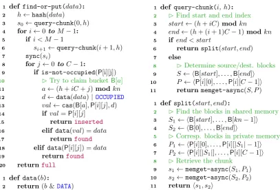
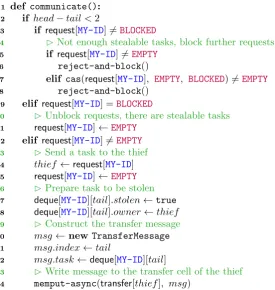
When a process queries a chunk, it transfers a consecutive block of C buckets from B into its private arrayP, so that the bucket may be examined locally. Whenfind-or-put does not find the intended bucket, it may query for the next chunk. As a result, several consecutive chunks might be requested. The query-chunk(i, h) operation queries for the ith consecutive chunk, assuming i ≥ 0, starting from bucket B[h modkn]. The query-chunk operation returns a handle, which can be given tosync to synchronize on the query, which blocks further execution of the process until the roundtrip completes. By calling query-chunk multiple times before synchronizing on them, their queries overlap, thereby reducing the amortized waiting times.

(27)

chunks that are non-consecutive in memory. Two roundtrips are required to fetch them, which are performed bysplit(lines9and10). Thememget,memput, andsyncoperations are discussed in Section2.5.2.

3.4.3 Design Considerations of

find-or-put

Thefind-or-put(d) operation returnsfoundwhend∈T (lines17and19) before invoking the operation and returnsinsertedwhend6∈T(line15) before invoking the operation. Ifd6∈T and allM C consecutive buckets starting fromh(d) are already occupied,fullis returned (line20). In our implementation, the execution of the program simply terminates whenfull is returned, but it would also be possible to perform rehashing or resizing of the hash table. We did not implement either of the two schemes, since we allocate all available memory when using the hash table in the BDD implementation. This makes resizing superfluous. Furthermore, rehashing would only help slightly when the current hash function is replaced by a better, probably more computational intensive hash function. Figure3.2shows that the hash table is expected to easily handle load-factors up to 0.9 when a reasonable chunk size is used, which is enough for our use case.

Retrieving Chunks. The algorithm starts by requesting the first chunk (line3) and, if needed, tries a maximum of M −1 more chunks (line 4) to find the intended bucket. Before calling sync(si) on line7, the next chunk is already requested by callingquery-chunk(i+ 1, d) on line6.

This call returns a handlesi+1 and before this handle is synchronized on, first a whole iteration

of the for-loop at line 4 is performed. Such an iteration includes the synchronization of the previous query (with the exception of the first iteration) and the iteration over the chunk itself. This reduces overal waiting times. We actually expect queries to be already completed when synchronization is performed.

Iterating a Chunk. By iterating over a chunk in private memory, when some bucket P[i][j] is empty, find-or-put tries to insert data into that bucket with cas on line 13. B[a] is the bucket in shared memory corresponding toP[i][j] in private memory. The former value ofB[a] is returned by cas, which is enough to check if the casoperation succeeded (line 14). In that case, inserted is returned (line 15). Otherwise, some other process claimed B[a] in the time between the calls to query-chunk and cas. It might happen that dis written to that bucket, hence the check at line 16. If not,find-or-put returns to line 8 and tries the next bucket. If

P[i][j] is occupied, find-or-putchecks ifd∈P[i][j] at line18. In that case, foundis returned. If not, the next bucket is tried.

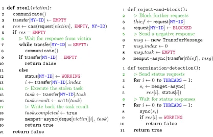
Interleaving Queries. Figure 3.6 shows the effect of performing asynchronous queries. The find-or-put(d) operation queries for the first and second chunk on lines3 and 6, respectively. It then synchronizes on the first chunk at line7, which causes the process to halt (shown by the gray bar atsync(s0)). After that, the first chunk is iterated. If the intended bucket is not found

(28)

1 def find-or-put(data): 2 h←hash(data)

3 s0←query-chunk(0, h)

4 fori←0toM −1: 5 if i < M−1

6 si+1←query-chunk(i+ 1, h)

7 sync(si)

8 forj←0 toC−1:

9 if is-not-occupied(P[i][j])

10 BTry to claim bucketB[a]

11 a←(h+iC+j)modkn 12 d←data(data)|OCCUPIED

13 val←cas(B[a],P[i][j], d) 14 if val=P[i][j]

15 returninserted

16 elif data(val) =data 17 returnfound

18 elif data(P[i][j]) =data 19 returnfound

20 returnfull

1 def data(b):

2 return(b&DATA)

1 def query-chunk(i,h):

2 BFind start and end index

3 start←(h+iC)modkn

4 end←(h+ (i+ 1)C−1)modkn 5 if end < start

6 returnsplit(start, end) 7 else

8 BDetermine source/dest. blocks

9 S← hB[start], . . . ,B[end]i

10 P← hP[i][0], . . . ,P[i][C−1]i

11 returnmemget-async(S, P)

1 def split(start, end):

2 BFind the blocks in shared memory

3 S1← hB[start], . . . ,B[kn−1]i

4 S2← hB[0], . . . ,B[end]i

5 BCorresp. blocks in private memory

6 P1← hP[i][0], . . . ,P[i][|S1| −1]i

7 P2← hP[i][|S1|], . . . ,P[i][C−1]i

8 BRetrieve the chunk

9 s₁←memget-async(S₁, P₁)

10 s₂←memget-async(S₂, P₂)

[image:28.595.97.505.100.376.2]

11 returnhs₁, s₂i

Figure 3.5: The design of find-or-put andquery-chunk. Thequery-chunk operation queries theith chunk andsync synchronizes on it. The 64-bit bitmaskOCCUPIEDdenotes bucket occu-pation andDATA masks data in a bucket.

3.5 Experimental Evaluation

We implemented the design of find-or-putin Berkeley UPC, version 2.20.0. The implementa-tion is evaluated by measuring latency, throughput, and the number of roundtrips required by find-or-put under various configurations. Furthermore, we compared the actual experimen-tal outcomes with our research expectations, which are given in Section 3.3. The experiments have been performed on a cluster of 10 Dell M610 machines (the m610 partition in the CTIT computing lab). Each machine has 8 CPU cores and 24 GB of internal memory. All machines run Ubuntu 14.04.2 LTS with kernel version 3.13.0 and are connected via a 20 GB/s Infiniband network. All experiments have been repeated at least three times, and the average measurements are considered.

(29)

partici-initiator

RDMA device of target

Main memory of target

s0=query-chunk(0, d)

s4=query-chunk(4, d) sync(s0)

sync(s1)

sync(s2)

sync(s3)

[image:29.595.133.457.102.320.2]

. . .

Figure 3.6: The effects of using query-chunk and sync-chunk to retrieve chunks of buckets asynchronously. The gray-striped rectangles denote the waiting time for the blockingsync-chunk operation to return. The white rectangles denote the time to iterate over theCbuckets, obtained by the previous call toquery-chunk.

pating machines. The-shared-heapenables every process to allocate up to 1100 MB of shared memory. The local benchmarks were executed viaupcrun -n threads -N 1 -pthreads threads -bind-threads, with theads the number of parallel UPC threads to use. The -bind-threads flag causes threads to be bound to CPU cores, which increases performance.

3.5.1 Throughput of

find-or-put

We measured the throughput of find-or-put in terms of operations per second (op/s). This is done by creating a shared hash table where each participating process contributes a block of 1024 MB. Thus, the total hash table size isp×210 _{MB, with}_p_{the total number of processes.}

Every process performs 107 _find-or-put_{operations with pseudo-randomized data.}

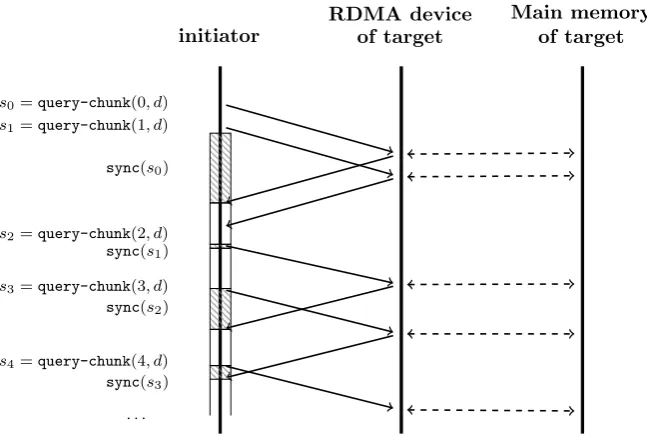
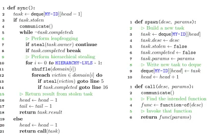
Three different workloads have been taken into account when measuring throughput, namely amixed workload (50% finds, 50% inserts), aread-intensive workload (80% finds, 20% inserts), and a write-intensive workload (20% finds, 80% inserts). For each workload, we used a differ-ent procedure to select the pseudo-randomized data given to each call to find-or-put. This procedure is able to introduce a skew in the workload if needed, while maintaining a proper distribution of data (i.e. the memory of every process is accessed equally often). Also, every process performs an approximately equal amount of finds and inserts.

(30)

1 2 4 6 8 10 2

3 4

·108

Threads

Throughput

(op/s)

(a) Throughput per thread

1 2 4 6 8 10

1 2

·109

Threads

Throughput

(op/s)

mixed read write

(b) Total throughput

Figure 3.7: Throughput of find-or-put using one machine (i.e. without using RDMA). The throughput is measured under a mixed workload, a read-intensive workload, and a write-intensive workload. The total throughput is the sum of the throughputs of all threads.

Workload Base Throughput Best Throughput Speedup

Throughput Procs. Throughput Procs.

Mixed 324,676,333 1 2,049,388,900 8 6.31

Read-intensive 376,434,000 1 2,342,278,333 7 6.22 Write-intensive 422,593,000 1 1,963,570,267 9 4.65

Figure 3.8: The throughputs obtained when using one machine. The throughputs obtained with one process (base throughputs) and the best achieved throughputs are given.

comparison with one thread. In that case, shared memory is used (i.e. memory shared between two threads), which causes a performance reduction compared to one thread. When more than 8 threads are used, performance also drops. This is because the machines used in the experiments only have 8 physical CPU cores. When considering a mixed workload, a maximum speedup of 6.3 is reached when 8 threads are used (see also Figure3.8). Surprisingly, the benchmarks with a mixed workload obtain higher speedups than the read-intensive workloads. We expect this to be caused by the overhead generated due to asynchronous queries. We may conclude that asynchronous queries are more beneficial for remote operations. The write-intensive benchmarks obtain lower speedup because those operations fill buckets, in addition to merely reading neigh-bourhoods.

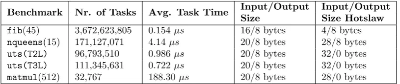
Remote Throughput. Figure3.10shows the average throughputs when RDMA is used by the processes. In addition, Figure3.12shows the best achieved throughputs for the different work-loads. Compared to the local throughputs, a performance drop of several orders of magnitude is observed. A peak-throughput of 2.05×109 _{op/s is reached locally under a mixed workload,}

(31)

1 2 4 6 8 10 1

2 3 4 5 6

Processes

Sp

eedup

mixed read write

Figure 3.9: Speedups on throughput when using one machine (i.e. without using RDMA). A mixed workload (mixed), a read-intensive workload (read), and a write-intensive workload (write) is considered.

the north-bridge, which impacts performance.

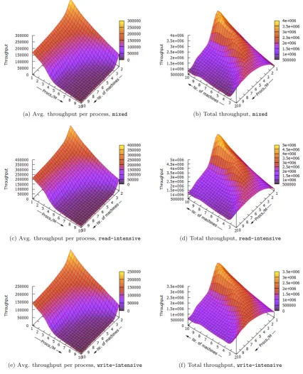
The average throughputs per process, shown in Figure 3.10, clearly shows the saturation points for the RDMA devices. When enough processes are added, the throughput per processes remains relatively linear. The relatively steep slope beforehand is caused by the many processes used per machine, which is a threshold for the RDMA devices to reach their maximum through-put. By default, Berkeley UPC has a fixed number of processes per machine, but we expect that this slope could be less steep when a variable number of processes per machine could be used instead. In addition, we expect that the maximum achievable throughput also increases by spawning processes dynamically. It would be interesting to try dynamic thread creation and apply algorithms thatlearnthe effects on performance when threads are either added or removed. The total throughputs, presented in the right plots in Figure 3.10, also show the saturation points of the RDMA devices. These results imply that scalability along CPUs decreases when the number of machines increases. Performance can only be improved by improving data-locality in some way, or by further minimizing the number of RDMA operations. Section 3.5.3 gives suggestions on how to potentiallydouble the achievable throughput. By reducing the number of roundtrips, more processes are needed to saturate the RDMA devices, but scalability remains an issue. Therefore, improving data-locality is key to support networks of many-core machines. Figure 3.11 presents the speedups obtained by the remote throughput benchmarks, which look very similar to the graphs shown in Figure3.10. The speedups are determined relative to two machines, each having one process. Again, we expect the steep slopes to become less steep when treads are dynamically created, adapting to performance differences.

3.5.2 Latency of

find-or-put

(32)

(a) Avg. throughput per process,mixed (b) Total throughput,mixed

(c) Avg. throughput per process,read-intensive (d) Total throughput,read-intensive

[image:32.595.93.520.125.652.2]

(e) Avg. throughput per process,write-intensive (f) Total throughput,write-intensive

Distributed Symbolic Reachability Analysis