Semi parametric dynamic time series modelling with applications to detecting neural dynamics

University of Warwick institutional repository: http://go.warwick.ac.uk/wrap

This paper is made available online in accordance with

publisher policies. Please scroll down to view the document

itself. Please refer to the repository record for this item and our

policy information available from the repository home page for

further information.

To see the final version of this paper please visit the publisher’s website

.

Access to the published version may require a subscription.

Author(s): F Rigat and JQ Smith

Article Title: Sequential change-point detection for time series models:

assessing the functional dynamics of neuronal networks

Year of publication: 2007

Link to published article:

http://www2.warwick.ac.uk/fac/sci/statistics/crism/research/2007/paper

07-7/

Semi-parametric dynamic time series modelling

with applications to detecting neural dynamics.

Fabio Rigat∗

Jim. Q. Smith†

October 1st, 2008

Abstract

This paper illustrates the theory and applications of a methodol-ogy for non-stationary time series modeling which combines sequen-tial parametric Bayesian estimation with non-parametric change-point testing. A novel Kullback-Leibler divergence between posterior dis-tributions arising from different sets of data is proposed as a non-parametric test statistic. A closed form expression of this test statistic is derived for exponential family models whereas Markov chain Monte Carlo simulation is used in general to approximate its value and that of its critical region. The effects of detecting a change-point using our method are assessed analytically for the one-step ahead predictive distribution of a linear dynamic Gaussian time series model. Condi-tions under which our approach reduces to fully parametric state-space modeling are illustrated.

The method is applied to estimating the functional dynamics of a wide range of neural data, including multi-channel electroencephalo-gram recordings, the learning performance in longitudinal behavioural experiments and in-vivo multiple spike trains. The estimated dynam-ics are related to the presentation of visual stimuli, to the generation of motor responses and to variations of the functional connections be-tween neurons across different experiments.

Introduction

Stochastic modeling of dynamic processes is often implemented via mod-els having time-dependent parameters (Hamilton [1994], West and Harrison

∗_{CRiSM, Department of Statistics, University of Warwick; [email protected]}

[1997], Fr¨uhwirth-Shnatter [2006]). These dynamic time series models can effectively capture non-stationarities induced by the occurrence of change-points in the data dependence structure (Page [1955], Smith [1975], Carlin et al. [1992], Ferger [1995], Chib [1998]), by switches among different depen-dence regimes (Hamilton [1990], Shumway and Stoffer [1991], Robert et al. [1993], Albert and Chib [1993], McCulloch and Tsay [1994], Kim [1994],

Ghahramani and Hinton [2000], Fr¨uhwirth-Shnatter [2001]) or by smooth

changes of the model parameters through time (Harrison and Stevens [1976], West and Harrison [1986a]). This paper illustrates the theory and applica-tions of a novel sequential method for estimating semi-parametrically the dynamics of such time-dependent model coefficients.

The distinctive characteristic of our approach with respect to state-space and hidden Markov models (Kalman [1960], West et al. [1985], West and Harrison [1997], Cappe et al. [2005]) and parametric change-point models (Muller [1992], Stephens [1994], Loader [1996], Mira and Petrone [1996], B´elisle et al. [1998], Jain et al. [2007], Fearnhead and Liu [2007]) is that change-points are defined through the discrepancy between one-step ahead predictive distributions, measured here by a novel Kullback-Leibler (KL) divergence (Kullback and Leibler [1951], Kullback [1997]). The distribution of this KL statistic reflects the concentration of the joint posterior distribu-tion of the model’s parameters when new data are generated using the same model structure as for past observations and parameter values drawn from their current joint posterior distribution. An important implication of this approach is that the occurrence of changes in the model coefficients is not assumed as in standard state-space frameworks but it is sequentially tested at each time point.

The motivation for adopting this sequential framework for dynamic time series modeling is twofold. First, in state-space models inferences and

pre-dictions are sensitive to the form of the state evolution equations (Fr¨

uhwirth-Shnatter [1995], Bengtsson and Cavanaugh [2006]). Therefore, an exploratory non-parametric approach is a natural choice for a first analysis of the data when no reliable information about the latent evolution of a model’s

parame-ters are available (Robinson [1983], H¨ardle et al. [1997]). This is typically the

practical alternative providing a non-parametric point estimate of a latent change-point process without computing marginal likelihoods.

Section 1 of this paper includes the methodological developments. A general time series framework is introduced and the KL test is illustrated. A closed form expression of the KL statistic for exponential family models is derived and examples are presented. Markov chain Monte Carlo simulation (Gelfand and Smith [1990], Tierney [1994]) is used to estimate in general the value of the KL statistic and of its critical region under the null hy-pothesis. A sequential algorithm integrating parametric Bayesian inference with a non-parametric change-point test using the KL statistic is presented. The behaviour of both location and spread of the one-step ahead predictive distribution is described analytically as a function of the timing of the last detected change-point for a linear Gaussian dynamic model with conjugate priors. Conditions are given so that our semi-parametric approach reduces to fully parametric state-space modeling.

In sections 2, 3 and 4 our method is applied to estimating three differ-ent types of neural dynamics. First we analyse a multivariate time series of electroencephalogram (EEG) recordings (Delorme et al. [2002], Makeig et al. [2002]) to reconstruct the dynamics functional relationships among different brain areas. Second, we estimate semi-parametrically a learning curve using a univariate binary time series arising from a longitudinal behavioural ex-periment (Smith et al. [2004]). Finally, our method is applied to estimating the functional dynamics of networks of neurons using in-vivo experimental

multiple spike trains recordings (Buzs´aki [2004]).

1

Sequential time series modelling and

Kullback-Leibler change-point testing

Let {Yi}Ni=1 represent a sequence of N consecutive time series Yi ∈ Y of

random variables Yi,k,t with k = 1, ..., K measured at the time points t =

ti,1< ti,2 < ... < ti,ni withti,ni< ti+1,1. The distinction between theN time

series is relevant when we allow for the occurrence of time gaps of possibly

unknown length between them. This situation arises, for instance, whenN

consecutive trials are run sequentially interposed by resting periods.

The marginal probability of the data (Y1 =y1, ..., YN =yn) can always

be written as

P(y1, ..., yN) = N Y

i=1

wherey0:(i−1)_{includes fixed initial conditionsy}0_{and the observations (y}

1, ..., yi−1)

(see, for instance Dawid [1984]). Explicit representations of the left-hand

side of (1) are obtained by specifying suitable conditional distributionsP1(y1|

y0), ..., PN(yN | y0:(N−1)). From a Bayesian perspective, these conditional

distributions are often constructed by assuming that

Pi(yi |y0:(i−1)) = Z

Θi

P(yi |θi−1, y0:(i−1))f(θi−1 |y0:(i−1))dθi−1, (2)

meaning that the multivariate time seriesYiare assumed to be generated by

a fixed model P(yi |θi−1, y0:(i−1)), such as a vector auto-regressive (VAR)

model with shared parameters θi−1 within each of the N periods. The

probability density f(θi−1 |y0:(i−1)) here represents the distribution of the

model coefficients given the initial conditionsy0 _{and all past observations.}

Note that in (2), although the parameter values are allowed to vary in time, neither the functional form of the likelihood function nor the interpretation of its coefficients change over time.

Within this framework, dynamic modeling consists of specifying a

trans-fer map taking as arguments the posterior densityf(θi−1 |y0:(i−1)), the time

series datayiand possibly additional hyper-parametersα and returning the

density f(θi | y0:i) for any value i = 1, ..., N. Various characterisations of

analogous maps are given, for instance, in Smith [1990] and Smith [1992]. In standard state-space models the coefficients are assumed to vary across each time period, so that their transfer map is defined implicitly via the

transition equations defining the prior distribution for θi in terms of the

coefficients θi−1 and of fixed hyper-parameters. In Markov switching and

finite mixture time series models, this transfer map is again derived from

modelling the full joint density of the coefficients θi and θi−1 conditional

on the location of a sequence of change-points (Fr¨uhwirth-Shnatter [2006]).

In this work we model the transfer map semi-parametrically by integrating sequential Bayesian inference for the model’s parameters with a statistic detecting the occurrence of change-points. The latter statistic is similar in spirit to the cumulative Bayes factors proposed in West [1986] and West and Harrison [1986b], with the practical advantage that the computation of marginal likelihoods is not required.

When a change-point occurs upon observing the data yi, we define a

transfer prior

θi ∼h(θi |θˆi−1), (3)

taking as arguments functionals of the current posterior density, ˆθi−1, and

many possible formulations of this transfer prior we let the hyperparameters

of the conditional prior density for θi be fully specified using estimates of

the first two moments of the current posterior density. We note that similar forms of prior moment matching have been used for dynamic point process modeling by Gamerman [1992] and for multi-process dynamic linear models by West and Harrison [1997].

Equation (3) represents a partially specified state evolution density where neither the exact form of the prior nor the time of occurrence of the change-points are given a priori. Specific choices for the prior density will in fact depend on the structure of the time series model being entertained and on the interpretation of its parameters. When no change-points are detected

prior to observing the dataYi =yi, under (3) the joint posterior density of

the model’s parameters is

f(θi |y0:i, α)∝ (

f(θi−1|y0:(i−1))P(yi |θi−1, y0:(i−1)) if yi∈Ψi(α), h(θi |θˆi−1)P(yi |θi, y0:(i−1)) ifyi∈/ Ψi(α),

(4)

where Ψ1(α) =Y and for i= 2, ..., N the sets Ψi(α) ⊆ Y include the time

seriesYi which are inconsistent with their observed past under the assumed

model and the hyper-parametersα.

The implementation of (4) presents two related challenges. First, it is

essential to reformulate the rejection sets (Ψ2(α), ...,ΨN(α)) in terms of a

low-dimensional statistic and of the hyper-parameters α. Second, it must

be possible to derive the distribution of such statistic over the sample space at least approximately, so as to provide a sequential approximation of the

rejection sets for any value ofα. A natural way to overcome these challenges

is to view the sets (Ψ2(α), ...,ΨN(α)) as the α-level critical regions of a

sequential change-point test based on an appropriate statistic. The transfer map is thus completely specified by the transfer prior (3) together with a choice of this test statistic. The next section illustrates the derivation of a suitable statistic using well established information theoretic principles.

1.1 A Kullback-Leibler change-point statistic

The statistic proposed in this work has an analogous function to the KL divergence when used to support model selection. In the latter case, the null hypothesis specifies an assumed model structure which is compared to a typically more parsimonious formulation. In (4), under the hypothesis of no change sequential Bayesian learning is used to update the joint distri-bution of the model parameters. When this hypothesis is not sufficiently supported by the data, their distribution is updated using the conditional transfer prior (3). Therefore, instead of testing which of two competing model structures best predicts one given set of data, we construct a statistic detecting whether the same parameter values could have likely generated two sets of data given a common model structure.

As a statistic to measure the evidence in the data in favour of the hy-pothesis of no change we adopt a Kullback-Leibler divergence

KL(y0:(i+1)_{) =}R

Θilog

_f

(θi|y0:i₎

f(θi|y0:(i+1)₎

f(θi |y0:i)dθi,

= log(Eθi|y0:i(P(y_i+1|θ_i, y0:i)))−E_θi|y0:i(log(P(y_i+1 |θ_i, y0:i))), (5)

where the expectations in (5) are taken with respect to the posterior density

f(θi|y0:i). The right-hand side of (5) is finite when the likelihood function

is bounded away from zero for all values of the model’s parameters and when their posterior density is proper. In this case (5) is a non-negative convex function measuring the discrepancy between the posterior densities

f(θi|y0:i) andf(θi|y0:(i+1)), being equal to zero if and only if the likelihood

function does not vary withθiover the range of the former posterior density.

Prior to observing the data Yi+1 = yi+1, (5) is a random variable which

distribution under the null hypothesis depends on that of the future data

Yi+1via the time series modelP(Yi+1 |θi, y0:i). The following sections focus

on the interpretation and on the computation of (5).

1.1.1 Interpretation of the KL statistic and of the change-points

The hyper-parameter α of the joint posterior (4) has the interpretation of

the type-1 error probability for the change-point test using the statistic (5).

The rejection sets can be written explicitely as intervals Ψi(α) = (li,α, ui,α),

each representing the α-level highest probability interval for the random

variable (5) under the hypothesis of no change over periodi.

When (5) lies below the value li,α, the likelihood is almost a constant

function of the parametersθifor non-negligible values of their current

poste-rior density. In other terms, the parameter values maximising the likelihood

probability by the posterior distribution under the hypothesis of no change.

If the change-point statistic lies above ui,α, the parameter values

maximis-ing the likelihood of the datayi+1are associated to substantial values of the

current joint posterior density but they are far from its global maximum. In

this case the joint posterior density of all datay0:(i+1) _{under the hypothesis}

of no change tends to be bimodal, signaling that the latest batch of data

yi+1 are not adequately explained by the current parameter values.

In both the above cases, the detection of change-points using the statistic

(5) indicate that, with probability 1−α, the estimated shape of the

pos-terior density ofy0:(i+1) _{significantly departs from its assumed shape under}

the hypothesis that standard sequential Bayesian inference is adequate for estimating the model parameters in time.

When α = 0 no change-point is ever detected, so that the only

revi-sions in the estimates of the model’s parameters are those induced by the

sequential accrual of information via Bayes’ rule. On the other end, ifα= 1

a change-point in the parameter values is systematically detected at every time point. In this second limiting case the methodology proposed in this work is equivalent to a fully parametric first order Markov state-space model with state evolution equation partially specified by the transfer prior (3).

1.1.2 Computation of the change-point statistic

In general neither the value of (5) nor the rejection sets (Ψ2(α), ...,ΨN(α))

can be derived in closed form under the hypothesis of no change. At each

time period i = 2, ..., N this change-point statistic and its critcal interval

can be approximated using a sequence of draws{θm

i }Mm=1 generated using a

Markov chain Monte Carlo algorithm (Gelfand and Smith [1990], Smith and Roberts [1993], Tierney [1994]) having as target the posterior probability

density of the model’s parameters at period i conditional on the

change-points detected in the past. Using this technique, the value of (5) can be approximated using the average

KL(y0:(i+1))≈log

PM

m=1P(yi+1 |θmi , y0:i) M

!

−

PM

m=1log(P(yi+1 |θim, y0:i))

M . (6)

An approximation of the distribution of (5) for varying values ofYi+1 under

the hypothesis of no change can be constructed using the same sequence of draws as follows:

i) for each draw θm

i generate a pseudo-realisation ymi+1 using the joint

ii) compute the statistic KL(ym0:(i+1)), where ym0:(i+1) = (y0, ..., yi, yim+1),

using its Monte Carlo approximation (6).

The empirical distribution of the sequence{KL(ym0:(i+1))}Mm=1 approximates

that of the KL statistic (5) under the hypothesis of no change. Therefore

the empirical (α

2,1 − α2)th percentiles of the sequence {KL(y

0:(i+1)

m )}M_m=1

approximate the rejection sets Ψi(α) = (li,α, ui,α) for any given value ofα.

1.2 Sequential fitting and change-point testing algorithm

Given initial conditions (α, y0) and a parametric time series modelP(Yi+1|

θi, y0:i), time-dependent inferences for its coefficients θi can be derived by

integrating Bayesian sequential learning with the change-point KL test de-scribed above. We illustrate this algorithm starting from the first sample y1:

i) upon observing the datay1, derive the posterior density

f(θ1 |y0:1)∝h(θi |y0)P(yi |θi, y0),

ii) having observed datay2, compute the statisticKL(y0:2) and its

rejec-tion set Ψi(α) = (l1,α, u1,α) as described in the previous section;

iii) if l1,α< KL(y0:2)< u1,α, update the posterior density as

f(θ1|y0:2, α) ∝f(θ1|y0:1)P(y2 |θ1, y0:1).

Otherwise, derive the conditional posterior density

f(θ2 |θˆ1, y0:2, α)∝h(θ2|θˆ1)P(y2 |θ2, y0:1),

where ˆθ1 represents estimates of the first two moments of the f(θ1 |

y0:1_).

In the latter case, the sequentially estimated process of change-points up to

and including times (1,2) reports one change at time 2. Consistently with

the interpretation of the KL statistic, the model parameters are iteratively re-estimated using all data starting from the last detected change-point, if

any. When a change is detected at level 1−α, the new parameter values

1.3 Change-point KL statistic for exponential family models

The properties of the KL divergence within the exponential family have been explored by McCulloch [1988]. Also the divergence (5) has a closed

form when the dataYi is generated by an exponential family model. In this

case stochastic simulation is necessary to approximate only the value of the

interval Ψi(α) = (li,α, ui,α) under the hypothesis of no change. Without loss

of generality, in what follows we assume that no change-point is detected

prior to priodiand we letYibe a 1×ni dimensional sample of conditionally

independent observations with joint density (Diaconis and Ylvisaker [1979])

P(Yi |θi) = ni

Y

j=1

a(Yi,j)eYi,jθi−b(θi), (7)

whereθi is a scalar canonical parameter. Diaconis and Ylvisaker [1979] show

that each elment ofYi has mean and variance

E(Yi,j |θi) = ∂b(θi)

∂θi

, V(Yi,j |θi) =

∂2b(θi) ∂θ′_i∂θi

.

Using the prior

f(θi |n0, y0) =c(n0, S0)eS0θi−n0b(θi),

where S0 = n0y0 for scalar n0 and y0, the posterior for θi given the past

datay0:i _{has conjugate density}

f(θi|n(i), y0:i) =c(n(i), S(i))e

n(i)“_nS₍(i_i))θi−b(θi)

”

(8)

where n(i) = Pi

j=0nj, S(i) = Pji=0njy¯j and ¯yj represents the arithmetic

mean of sampleyj. Using the results of Guti´errez-Pe˜na [1997], the posterior

mean and variance ofθi are

E(θi |n(i), S(i)) =

∂H(n(i), S(i))

∂S(i) , V(θi |n(i), S(i)) =

∂H(n(i), S(i))

∂S(i)2 ,

and the posterior mean and variance of the functionb(θi) are

E(b(θi)|n(i), S(i)) =

∂H(n(i), S(i))

∂n(i) , V(b(θi)|n(i), S(i)) =

∂H(n(i), S(i))

∂n(i)2 ,

whereH(n(i), S(i)) =−log (c(n(i), S(i))). Using these results we can derive

theorem.

Theorem: When the posterior density for the coefficients θi has form (8),

given the data up to and includingyi+1 the Kullback-Leibler statistic (5) is

KL(y0:(i+1)) = log

c(n(i), S(i))

c(n(i+ 1), S(i+ 1))

−Si+1

∂H(n(i), S(i))

∂S(i) +

+ ni+1

∂H(n(i), S(i))

∂n(i) , (9)

where the terms on the right hand side of (9) are defined above.

Proof: by letting the posterior densities f(θi | n(i), S(i)) and f(θi |

n(i+ 1), S(i+ 1)) have form (8), the KL (5) becomes

KL(y0:(i+1)) = log

c(n(i), S(i))

c(n(i+ 1), S(i+ 1))

−Si+1E(θi) +ni+1E(b(θi)).(10)

For exponential family models, the expectations ofθi andb(θi) with respect

tof(θi |y0:i) in equation (10) are given in Guti´errez-Pe˜na [1997], as reported

above. By substituting these expressions in (10), equation (9) obtains. ⋄

Example 1.1: when Yi is a Gaussian random variable with mean µi

and precision λi, its distribution can be written in the form (8) using the

two-dimensional statistic

Y_i∗ = [Yi, Yi2],

and the canonical parameter

θi = [θ1,i, θ2,i] =

λiµi,− λi

2

.

with

a(Y_i∗) = (2π)−12,

b(θi) = = −

1

2log(−2θ2,i)−

θ₁2_,i θ2,i .

The conjugate prior for (µi, λi) is Normal-GammaN(µi |γ, λi(2α−1))Ga(λi |

α, β) with coefficients α > 0.5, β > 0, γ ∈ R and normalising constant

(Bernardo and Smith [2007])

c(n0, S0) =

2π

n0

1₂ 1

2S

S_1,0

2

2,0

Γ n0+1

2

where n0 = 2α −1, y0∗ = [y∗1,0, y2∗,0] = [γ,2α2−β1 +γ2], S1,0 = n0y1∗,0 and

S2,0 = n0y2∗,0. Upon observing the realisation (y1, ..., yi), the normalising

constant of the corresponding conjugate posterior is

c(n(i), S(i)) =

2π

n(i) 1₂ 1

2S(2, i)

S(1,i) 2

Γn(i₂)+1

,

wheren(i) =n0+i, S(1, i) =S1,0+Pji=1yj and S(2, i) =S2,0+Pij=1y2j.

When alsoyi+1 is observed, using (9) the KL statistic can be written as

KL(y0:(i+1)_{) = log} Γ

“

n(i+1)+1 2

”

Γ“n(i₂)+1”

!

+1₂logn(_ni₍+1)_i) + log

S(2,i)S(12,i)

S(2,i+1)S(1,i2+1)

−

−yi+1

2 log

S(2,i)

2

−y2_i+1S_S(1₍₂,i_,i)₎ +_2n1_(i) + Γn(i₂)+1∂Γ

“_n(i)+1

2

”

∂n(i) .

Example 1.2: let Yi be a sample of size ni of conditionally independent

Bernoulli random variables with success probabilities{πi}Ni=1. The canonical

representation of the Bernoulli probability mass function obtains by letting

θi = log

πi

1−πi

, b(θi) = log 1 +eθi

and a(Yi) = 1. The conjugate prior

for πi is Beta(S0, m0) where m0 = n0 −S0. Upon observing (y1, .., yi)

the conjugate posterior is Beta(S(i), m(i)), where S(i) =Pi

j=0Sj, n(i) = Pi

j=0nj andm(i) =n(i)−S(i). When alsoyi+1is observed, the KL statistic

(9) has form

KL(y0:(i+1)) = log

Qni

k=1(n(i) +k)

Qni−Si

w=1 (n(i)−S(i) +w)

QSi

j=1(S(i) +j)

!

−

−Si+1

Γ(S(i))

Γ(n(i)−S(i))

∂Γ(n_Γ((i_S)−_(iS₎₎(i))

∂S(i) +ni+1

∂(Γ(n(i))Γ(n(i)−S(i)))

∂n(i)

Γ(n(i))Γ(n(i)−S(i))).

Example 1.3: letYirepresent the random number of events of a given kind

observed within a time interval (ti,1, ti,ni] of fixed length. For this example

we assume that the latter is identical for all samples i= 1, ..., N. Let the

random times at which the events take place be distributed according to a

homogeneous Poisson process with intensity λi, so that the distribution of

Yi is Poisson with parameter λ∗_i = λi(ti,ni −ti,1). The canonical form of

the Poisson distribution has parameter θi = log(λ∗i) and functions a(Yi) =

1

Yi!, b(θi) = e

θi_{. The conjugate prior for λ}∗

i is Gamma with parameters

conjugate posterior forλ∗_i isGa(S(i), n(i)) withS(i) =S0+Pij=1yj,n(i) =

n0+i. When also yi+1 is observed, using (9) the KL statistic has form

KL(y0:(i+1)) = log S(i)n(i)

S(i)

n(i+ 1)S(i+1)

!

+yi+1



log(n(i))−

∂Γ(S(i))

∂S(i)

Γ(S(i))



−

S(i) n(i).

1.4 Effect of change-points for predictive densities

In this section we illustrate analytically the effect of detecting a change-point on the one-step ahead predictive density using the transfer prior (3) and a conjugate Gaussian model. As in the previus section, a univariate

time series is considered so that K = 1 and ni = 1 for all i = 1, ..., N.

For each value of i, in what follows we let Yi be distributed as N(µi, σ2i).

Analogously to example 1.1 in the previous section, the prior distribution

forθi = (µi, σi2) is taken as the conjugate form

µi ∼N(ˆµi∗₋₁, σ_i2),

σ_i2∼IGa(ν

2,

ν

2σˆ

2

i∗₋₁),

where 1≤i∗ < iis the time of the last detected change-point and (ˆµi∗₋₁,σˆ_i2∗₋₁)

represent the estimated mean and variance of the joint posterior density at

timei∗. Ifi∗ = 1, (µ0, σ02) represents a fixed initial condition. The variance

here has marginal inverse Gamma prior with density

f(σ2_i |ν,σˆ2_i∗₋₁) =

(ν₂σˆ2_i∗₋₁)

ν

2

Γ(ν₂) σ

−2(ν

2+1)

i e

−νσˆ

2

i∗ −1 2σ2

i .

Under this formulation, the prior expectation of the mean is ˆµi∗₋₁ and that

of the variance is ν2

ν

2−1σˆ

2

i∗₋₁. If follows that the one-step ahead marginal

predictive distribution is non-central Student-t. In absence of a

change-point previous to timei, the predictive density is

Yi+1 |y1:i, µ0, σ02∼tν+i

˜ µi,

i+ 1

i+ 2

ν+i

2 1 ˜ σ_i2

, (11)

where

˜

µi =

1

1 +iµ0+

i

1 +iy¯

(1:i)_,

˜

σ_i2 = ν

2σ 2 0 + i 2s 2 (1:i)+

i

i+ 1(µ0−y¯

and (¯y(1:i)_{, s}2

(1:i)) represent respectively the sample mean and variance of

the datay1:i_{. If a change-point is detected by the KL statistic (5) at time}

1< i∗ _{< i, under the transfer prior (3) the conditional predictive density is}

Yi+1|µˆi∗₋₁,σˆ_i2∗₋₁, yi ∗_:i

∼tν+i−(i∗₋₁₎

˜ µ∗_i,i−i

∗_{+ 2}

i−i∗_{+ 3}

ν+i−i∗+ 1

2

1

(˜σ2_i)∗

,(12)

where

˜

µ∗_i = 1

i−i∗_{+ 2}µˆi∗−1+

i−(i∗₋₁₎

i−i∗_{+ 2} y¯

(i∗_:i)

,

(˜σ_i2)∗ = ν

2(ˆσi∗−1)

2₊i−(i∗−1)

2 s

2 (i∗_:i)+

i−(i∗₋₁₎

i−i∗_{+ 2} (ˆµi∗−1−y¯

(i∗_:i)

)2.

Since the mean and variance of the non-central Student-t random variable

with density tν(µ, σ2) are respectively equal to µ and to _ν+2ν σ2, equations

(11) and (12) provide a characterisation of the one-step ahead posterior predictive moments as a function of the time of the last detected

change-point and of the inverse-Gamma prior coefficientν. Fori∗ >1 the predictive

mean is less influenced by the sample mean of the data preceding the

change-point, ¯y1:(i∗₋₁₎

, and it is more influenced by ¯yi∗_:i

, that is the sample mean of the data from the change-point on. When a change-point is detected the predictive variance is larger with respect to the case of no change. Its

relative increase is a decreasing function of the difference (i−i∗_{) and it is}

an increasing function of the coefficient ν, which measures the strenght of

the prior at the initial time.

This behaviour is consistent with the intuition that predictions ensu-ing from a dynamic time series model should appropriately discount the information content of remote data and focus on more recent data when sig-nificant dynamics occur. In absence of an autoregressive model structure, as in the present section, the distinction between remote and recent data is entirely left to the timing of the detected change-points.

2

Analysis of multivariate EEG recordings

Previous analyses of these data have emphasized an increased synchroniza-tion of different brain areas during the generasynchroniza-tion of the motor response to the visual stimulus. Here we use this data to investigate the relationships among seven functionally distinct brain areas. The multidimensional EEG time series are modeled as a discrete time Gaussian stochastic process, which randomness is thought of as arising from the intrinsic variability of the brain activity and from the presence of experimenatal artifacts.

The recordings from all cranial EEG channels are first averaged within each brain area for each trial. The rationale for this data reduction pre-processing is that the variability across trials of the EEG recordings within each brain region is small. The main features of the trial-averaged EEG recordings are illustrated in the top-left plot of Figure 1. The activity of the different brain areas prior to the presentation of the visual cue appears to be tightly synchronised, exhibiting a markedly periodic pattern occurring respectively at 10Hz and 60Hz for all seven areas. The lower frequency is

consistent with the so-called α band, reflecting eye movements. The higher

frequency is an experimental artifact suggestive of poor electrode grounding.

The seven-dimensional trial-averaged signal at timei,Yi, is modelled as

N7(µi,Σi). To derive Bayesian inferences for the mean vector and for the

covariance matrix, we use the conjugate Normal-Inverse-Wishart prior:

µi∼N7(ˆµi∗₋₁,Σ_i), (13)

Σi∼IW7(9,Σˆi∗₋₁), (14)

where 1≤i∗ _{< iis the time index of the last detected change-point prior to}

timei. The marginal prior expectations are matched to the corresponding

estimated posterior moments (ˆµi∗₋₁,Σˆ_i∗₋₁) consistently with the transfer

prior (3). The initial conditionsµ0and Σ0 were set respectively equal to the

null vector and to the identity matrix. The hyper-parameter of the posterior

density was set atα= 0.01 so as to dectect only the most prominent changes.

The number of degrees of freedom of the Inverse Wishart density is set so

that predictive intervals of length consistent with the set value ofα are not

excessively inflated when a change is detected. The distribution of the KL

statistic and its value were approximated at each timei using the last 500

Gibbs sampler draws of the mean and of the covariance matrix.

shift in brain activity taking place roughly at half of the initial phase of the experiment, followed by a sharp increase corresponding to the cue pre-sentation, a down-ward trend in the activity following the motor response and a stabilisation of the EEG signals towards the end of the experiment. The sharp increases in the activity of the frontal and central areas during the generation of the response are consistent with their characterisation as executive and motor centres of the brain.

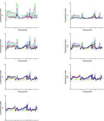
Figure 2 depicts the estimates of the time-dependent variance and covari-ance functions for each brain area. Whole segments represent periods dur-ing which their 95% highest posterior intervals do not intersect zero. All estimated variances and covariances vary over time, indicating that a time-dependent covariance matrix is an appropriate modelling assumption for this data. All estimated covariances are positive, suggesting that the activ-ity of the seven brain areas is dynamically cooperative as found by Delorme et al. [2002]. The covariances between most brain areas are increased upon detecting a change-point, suggesting a temporary increase in their mutual coordination. An important feature of the estimated covariance functions is their spatial ordering over time, the strongest relationships being esti-mated between adjacent brain areas. Since neither in the Gaussian likelihood nor the priors (13) include a spatial component, these estimates suggest a close correspondence between the detected functional relationships and the anatomical structure of the brain.

3

Estimation of a learning curve

0 50 100 150 200 250 300 350 400 0 5 10 15 20 Trial period EEG recordings

l l ll l l l −5 0 5 10 15 20 25 Trial period

Data and predictions area

F

l l ll l l l −5 0 5 10 15 20 25 Trial period

Data and predictions area

T

l l ll l l l −5 0 5 10 15 20 25 Trial period

Data and predictions area

C

l l ll l l l −5 0 5 10 15 20 25 Trial period

Data and predictions area

CP

l l ll l l l −5 0 5 10 15 20 25 Trial period

Data and predictions area

P

l l ll l l l −5 0 5 10 15 20 25 Trial period

Data and predictions area

PO

l l ll l l l −5 0 5 10 15 20 25 Trial period

Data and predictions area

O

l l ll l l l −5

0 5 10

Trial period

Covariances area

F

l l ll l l l −5

0 5 10

Trial period

Covariances area

T

l l ll l l l −5

0 5 10

Trial period

Covariances area

C

l l ll l l l −5

0 5 10

Trial period

Covariances area

CP

l l ll l l l −5

0 5 10

Trial period

Covariances area

P

l l ll l l l −5

0 5 10

Trial period

Covariances area

PO

l l ll l l l −5

0 5 10

Trial period

Covariances area

O

The data analysed in this section consist of a sequence of 55 binary tri-als during which a macaque monkey performed a location-scene association task (Wirth et al. [2003]). The learning curve is represented by the time-dependent estimates of the trials’success probabilities. We derived these estimates using a uniform prior for the success probability of the first trial. The transfer prior (3) was implemented using a conjugate Beta prior. The

hyper-parameterαwas set at 0.7, requiring weak evidence in order to detect

a change-point. This hyper-parameter setting was mainly motivated by the limited amount of data available for the analysis. The distribution of the KL statistic under the null hypothesis of no change was approximated using ten thousand Monte Carlo samples from the Beta posterior distribution of each trial’s success probability. For this data, the unsmoothed state-space esti-mates of Smith et al. [2004] suggest that, with 90% confidence, the success

probability significantly exceed its chance value 0.25 from trial 24 onwards.

Figure 3 shows that our estimates of the success probability are more conser-vative suggesting that, with 90% conditional posterior probability, learning has taken place from trial 29 onwards.

5 10 15 20 25 30 35 40 45 50 55

0 0.1 0.2 0.3 0.4 0.5 0.6 0.7 0.8 0.9 1

Time

Success Probability

Trial 29

4

Dynamic modelling of functional neuronal

net-works

This example illustrates the application of the method presented in section 1 in the context of a model for networks of spiking neurons. Introductions to the neuronal physiology and to neuronal modelling are presented in Fien-berg [1974] and Brillinger [1988]. Recent surveys of the state-of-the-art in multiple spike trains modelling can be found in Iyengar [2001], Brown et al. [2004], Kass et al. [2005], Okatan et al. [2005], Rao [2005] and Rigat et al. [2006]. Dynamic point process neuronal models based on fully parametric state-space representations have been proposed by Eden et al. [2004], Truc-colo et al. [2005], Brown and Barbieri [2006], Srinivansan et al. [2006] and Eden and Brown [2008].

During the experiments analysed in this section part of the neural activ-ity of a sheep’s temporal cortex is observed at discrete times. The goal of the experiments is to investigate the activity of brain areas associated with memory. At each experiment the sheep is shown either a blank screen or two images. In the latter case, a reward is given when one of a set of “familiar faces” is correctly identified. A sequence of 77 disconnected experimental in-vivo multi-electrode array (MEA) recordings is generated (Kendrick et al. [2001]).

4.1 A binary network model

In what follows each element of the experimental time series {Yi}77i=1 is

Yi,k,ti,j(i) = 1 if neuronk fires at time ti,j(i) during trial i and Yi,k,ti,j(i) = 0

otherwise withj(i) = 1, ..., ni. We model the joint sampling distribution of

the multiple spike data for trial i, Yi, as a Bernoulli process with renewal

(Rigat et al. [2006]). The joint probability of a given realisationyi is

P(Yi=yi|πi) = t_i,ni Y

t=ti,1 K Y

k=1

πyi,k,t

i,k,t (1−πi,k,t)

1−yi,k,t_{. (15)}

For model (15) to be biologically interpretable, the firing probability of

neuron k at time ti,j(i) during trial i, πi,k,ti,j(i), is defined as a one-to-one

non-decreasing mapping of a real-valued voltage functionvi,k,ti,j(i) onto the

interval (0,1). The functionvi,k,ti,j(i) represents the unnormalised difference

of electrical potential across the membrane of neuronk at time ti,j(i). Let

i, that is

τi,k,ti,j(i) = (

1 if Pti,j(i)

τ=1 Yi,k,τ = 0 or ti,j(i)= 1,

max{1≤τ < ti,j(i):Yi,k,τ = 1} otherwise,

and the voltage function is modelled as

vi,k,ti,j(i) = K X

l=1

βi,k,l

ti,j(i)−1 X

w=τ_i,k,ti,j(

i)

yi,l,w. (16)

The spiking probabilities are linked to (16) via the logistic mapping

πi,k,ti,j(i) =

evi,k,ti,j(i) 1 +evi,k,ti,j(i).

The coefficients βi,k,l represent the strenght of the functional relationship

from neuronl to neuronkduring triali. Whenβi,k,l is positive during trial

i, the firing activity of neuronl promotes that of neuronkwhereas when it

is negative firing ofl inhibits that of k. When k=l, the coefficients βi,k,k

represent the spontaneous spiking rate of neuron k during trial i. The last

summation term in equation (16) indicates that the membrane potential of a neuron is assumed to be influenced only by the spiking activity of the other neurons during its last inter-spike interval.

For each triali= 1, ..., N we use a Metropolis sampler to produce

approx-imate posterior inferences for the K2 _{model parameters. For each}

experi-ment, we run a random scan neuron-wise update with independent Gaussian random-walk proposals for twenty-five thousand iterations. The initial prior for the parameters of all experiments is Gaussian with zero mean, standard deviation 1 and zero covariance for all pairs of neurons. Conditionally on

the data y0:i _{and on the current posterior estimates, upon observing the}

outcome of theith+1 experiment, yi+1, we use the KL statistic (5) to test

whether a significant change occurred in any of the model’s parameters. The occurrence of such changes and the corresponding parameter estimates indicate statistically significant variations of different aspects of the neural activity.

4.2 Analysis of sheep multiple spike trains

activity of these 7 neurons during all 77 experiments. The panel on the right shows their mean firing rates, which reflect the overall low spiking frequency typical of this type of measurements. Brighter vertical bands mark experiments during which the mean firing rate for all neurons is relatively high. The co-occurrence of these high firing rates suggest that the most prominent connections among the seven neurons are mutually excitatory functional relationships.

0 1 2 3 4 5 6 7 x 104

0 1 2 3 4 5 6 7 8

Time

Number of spikes

Experiment number

Neuron number

10 20 30 40 50 60 70 1

2 3 4 5 6 7

0.02 0.03 0.04 0.05 0.06 0.07 0.08 0.09 0.1 0.11

Figure 4: spiking activity (left) and mean firing rates (right) for the 7 most active neurons among the 64 recorded cells. Each dot in the upper panel marks the number of spiking neurons for each millisecond of the 77 experiments. The range of the mean firing rates is 0.02−0.12, reflecting the low overall spiking frequency typical for this type of recordings. Vertical bright bands mark experiments during which the spiking activity of all neurons is relatively high, suggesting that the seven neurons are funciontally connected mostly via mutually excitatory relationships.

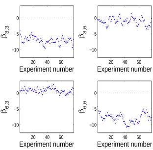
Figure 5 displays summaries of the point estimates of the network

coeffi-cients β across all experiments. The top-left panel shows the proportion of

65% of the experiments. Figure 6 illustrates in detail the point estimates and the 95% highest posterior intervals of this pair-wise connection together with those of each neuron’s self-dependence and of the connection from neuron 6 towards neuron 3. Consistently with the high proportion of experiments when it is found significant, the excitatory effect of neuron 3 to neuron 6 is the most stable estimate over time.

Neuron number

Neuron number

1 2 3 4 5 6 7 1 2 3 4 5 6 7 0 0.1 0.2 0.3 0.4 0.5 0.6 0.7 0.8 0.9 1 Neuron number Neuron number

1 2 3 4 5 6 7 1 2 3 4 5 6 7 0 0.1 0.2 0.3 0.4 0.5 0.6 0.7 0.8 0.9 1 Neuron number Neuron number

1 2 3 4 5 6 7 1 2 3 4 5 6 7 0 0.1 0.2 0.3 0.4 0.5 0.6 0.7 0.8 0.9 1

20 40 60 −10

−5 0

β

Experiment number

20 40 60

−10 −5 0

β

Experiment number

20 40 60

−10 −5 0

β

Experiment number

20 40 60

−10 −5 0

β

Experiment number

5

Discussion

This work is motivated by the difficulties encountered in constructing time series models when the niether the factors driving the dynamics of their pa-rameters nor the relationship between the resolution of the data and such dynamics are known. The semi-parametric method illustrated here provides flexible time-dependent estimates which may then suggest specific evolu-tion dynamics. For exploratory data analyses, such as those presented in sections 2, 3 and 4, these estimates may suffice to address specific scien-tific questions. Otherwise, appropriate measures of dependence between these time-dependent estimates and experimental factors of interest provide a principled basis for more precise formulations of the parameters’ dynam-ics. Describing the exact form of such dependence measures is very much context-dependent and it lies outside of the scope of this work.

A distinctive feature of the modeling approach proposed here is that it combines elements of sequential Bayesian learning and conditional frequen-tist inference along the lines of Guttman [1967], Box [1980], Berger et al. [1994], Meng [1994], Gelman et al. [1996], Berger and Bayarri [1997], Spiegel-halter et al. [2002], Bayarri and Morales [2003], Kuhnert et al. [2003] and Bayarri and Berger [2004] among others. A general treatment of such prag-matic combination of frequentist and Bayesian ideas for model criticism can be found in Chapter 8 of O’Hagan and Forster [1999]. From this perspective, our method is a “Bayesianly justifiable” procedure (Rubin [1984]) because only those future data that are consistent with the current conditional pos-terior distribution of the model parameters are relevant for approximating the distribution of the change-point statistic.

The latter statistic reflects a notion of a change-point as an observation which, on the basis of the chosen model with its prior and the observations so far, is ”surprising” from a predictive point of view. Note that this charac-terization does not depend on the parametrization of the state space nor on the unobservable sample paths of latent states, but it depends only on the predictives on observables. Defining models and their properties via their one step ahead predictive statements but has been recommended, among others, by Geisser and Eddy [1979] for predictive model selection, Dawid [1984] in his prequential inference, San Martini and Spezzaferri [1984] for model selection, West and Harrison [1986b] for monitoring the adequacy of Bayesian forecasting models and by Smith [1992] for comparing the charac-teristics of different forecasting models. More recently, optimal predictive model selection criteria have been proposed by Barbieri and Berger [2004].

param-eters is used to define their conditional posterior distribution. Should the data provide evidence of changes of only some parameters, the posterior distributions for the unchanging coefficients would not reflect an efficient use of the data. It is important to note that while in principle any subset of model parameters can be associated to a distinct change-point process, the limitations for implementing multivariate change-point process inference within our framework are eminently practical. This is because marginal like-lihoods for each subset of model parameters having a different change-point process are required to approximate the distribution of their change-point test statistic. For classes of models where marginal likelihoods are available in closed form, this work can be extended by introducing a random variable identifying groups of coefficients sharing a common change-point process.

Posterior simulation via Markov chain Monte Carlo algorithms has been used in this work to fit multivariate time series models and to approximate critical values of the KL statistic. Although the current implementation of our method is operationally realistic, these computationally intensive methods are in fact rather impractical for an iterative process of model formulation and criticism. Currently two directions are being pursued to improve the computational efficiency of our method. On the one hand, faster resampling methods such as particle filters (Doucet et al. [2001]) and approximate Bayesian computation (Marjoram et al. [2003]) can be adopted. Alternatively, analytical posterior approximations can be adopted (Tierney and Kadane [1986]). For instance, in the context of sequential time series modeling Koyama et al. [2008] recently proposed a Laplace-Gauss posterior approximation that obviates the use of cumbersome resampling techniques.

Acknowledgements

The Authors acknowledge the support of the Centre for Research in Statis-tical Methodology (CRiSM) at the University of Warwick, UK, during the development of this work.

We wish to thank Arnaud Delorme for sharing the EEG recordings anal-ysed in section (2), which are currently available at the URL:

http://www.sccn.ucsd.edu/~arno/fam2data/

References

H. Akaike. Likelihood of a model and information criteria.Journal of Econometrics, 16:3–14, 1981.

H. Akaike. On the likelihood of a time series model. The Statistician, 27:217–235, 1978.

J.H. Albert and S. Chib. Bayes inference via Gibbs sampling for autoregressive time series subject to Markov mean and variance shifts.Journal of Business and Economic Statistics, 11:1 – 15, 1993.

M.M. Barbieri and J.O. Berger. Optimal predictive model selection. The Annals of Statistics, 32:870–897, 2004.

M.J. Bayarri and J.O. Berger. The interplay between Bayesian and frequentist analysis. Statistical Science, 19:58 – 80, 2004.

M.J. Bayarri and J. Morales. Bayesian measures of surprise for outlier detection.

Journal of Statistical Planning and Inference, 111:3 – 22, 2003.

P. B´elisle, L. Joseph, B. MacGibbon, D.B. Wolfson, and R. du Berger. Change-point analysis of neuron spike train data. Biometrics, 54:113 – 123, 1998.

T. Bengtsson and J.E. Cavanaugh. An improved Akaike information criterion for state-space model selection.Computational Statistics and Data Analysis, 50:2635 – 2654, 2006.

J.O. Berger and M.L. Bayarri. Measures of surprise in bayesian analysis. ISDS Discussion Paper, 46, 1997.

J.O. Berger, L. Brown, and R.L. Wolpert. A unified conditional frequentist and Bayesian test for fixed and sequential hypothesis testing.The Annals of Statistics, 22:1787 – 1807, 1994.

J. Bernardo. Expected information as expected utility. The Annals of Statistics, 7: 686–690, 1979.

J.M. Bernardo and A.F.M. Smith. Bayesian theory. Wiley, 2007.

G. E. P. Box. Sampling and Bayes’ inference in scientific modelling and robustness.

Journal of the American Statistical Association A, 143:383–430, 1980.

D.R. Brillinger. Some statistical methods for random processes data from seismol-ogy and neurophysiolseismol-ogy. The Annals of Statistics, 16:1–54, 1988.

E.N. Brown and R. Barbieri. Dynamic analyses of neural representations using the state-space modeling paradigm. In: Madras, B., Von Zastrow, M. Colvis, C., Rutter, J. Shurtleff, D. and Pollock, J. eds. ”The Cell Biology of Addiction”, New York, Cold Spring Harbor Laboratory press, 2006.

G. Buzs´aki. Large scale recording of neuronal ensembles. Nature Neuroscience, 7: 446–451, 2004.

O. Cappe, E. Moulines, and T. Ryden. Inference in Hidden Markov Models. Springer, 2005.

B.P. Carlin, A.E. Gelfand, and A.F.M. Smith. Hierarchical Bayesian analysis of changepoint problems. Applied Statistics, 41:389–405, 1992.

C. Carota, G. Parmigiani, and N. Polson. Diagnostic measures for model criticism.

Journal of the American Statistical Association, 91:753–762, 1996.

S. Chib. Estimation and comparison of multiple change-point models. Journal of Econometrics, 86:221 – 241, 1998.

F. Critchley, P. Marriott, and M. Salmon. Preferred point geometry and the local differential geometry of the Kullback-Leibler divergence.The Annals of Statistics, 22:1587–1602, 1994.

A.P. Dawid. Present position and potential developments: some personal views. statistical theory: the prequential approach. Journal of the Royal Statistical Society A, 147:278–292, 1984.

A. Delorme, S. Makeig, M. Fabre-Thorpe, and T. J. Sejnowski. From single trial EEG to brain area dynamics. Neurocomputing, 44:1057–1064, 2002.

P. Diaconis and D. Ylvisaker. Conjugate priors for exponential families.The Annals of Statistics, 7:269–281, 1979.

A. Doucet, N. De Freitas, and N.J. Gordon. Sequential Monte Carlo Methods in Practice. Springer-Verlag, New York, 2001.

U.T. Eden and E.N. Brown. Continuous-time filters for state estimation from point process models of neural data. Statistica Sinica, 2008.

U.T. Eden, L.M. Frank, R. Barbieri, V. Solo, and E.N. Brown. Dynamic analysis of neural encoding by point process adaptive filtering. Neural Computation, 16: 971–998, 2004.

P. Fearnhead and Z. Liu. On-Line Inference for Multiple Change Points. Journal of the Royal Statistical Society B, 69:589–605, 2007.

S. E. Fienberg. Stochastic models for single neuron firing trains: a survey. Biomet-rics, 30:399–427, 1974.

S. Fr¨uhwirth-Shnatter. Bayesian model discrimination and Bayes factors for linear gaussian state-space models. Journal of the Royal Statistical Society B, 1:237 – 246, 1995.

S. Fr¨uhwirth-Shnatter. Markov chain monte carlo estimation of classical and dy-namic switching and mixture models. Journal of the American Statistical Asso-ciation, 96:194 – 209, 2001.

S. Fr¨uhwirth-Shnatter. Finite Mixture and Markov Switching Models. Springer, 2006.

D. Gamerman. A dynamic approach to the statistical analysis of point processes.

Biometrika, 79:39–50, 1992.

S. Geisser and W.F. Eddy. A predictive approach to model selection. Journal of the American Statistical Association, 74:153 – 160, 1979.

A.E. Gelfand and A. F. M. Smith. Sampling-based approaches to calculating marginal densities. Journal of the American Statistical Association, 85:398–409, 1990.

A. Gelman, X.L. Meng, and H.S. Stern. Posterior predictive assessment of model fitness via realized discrepancies. Statistica Sinica, 6:733–807, 1996.

Z. Ghahramani and G.E. Hinton. Variational learning for switching state-space models. Neural Computation, 12:831 – 864, 2000.

C. Goutis and C. Robert. Model choice in generalised linear models: A Bayesian approach via Kullback-Leibler projections. Biometrika, 85:29–37, 1998.

E. Guti´errez-Pe˜na. Moments for the canonical parameter of an exponential family under a conjugate distribution. Biometrika, 84:727–732, 1997.

I. Guttman. The use of the concept of a future observation in goodness-of-fit problems. Journal of the Royal Statistical Society B, 29:83 – 100, 1967.

P. Hall. On Kullback-Leibler loss and density estimation.The Annals of Statistics, 15:1491–1519, 1987.

J.D. Hamilton. Time Series Analysis. Princeton University Press, 1994.

J.D. Hamilton. Analysis of time series subject to changes in regime. Journal of Econometrics, 45:39 – 70, 1990.

W. H¨ardle, H. L¨utkepohl, and R. Chen. A review of nonparametric time series analysis. International Statistical Review, 65:49 – 72, 1997.

P.J. Harrison and C.F. Stevens. Bayesian forecasting. Journal of the Royal Statis-tical Society B, 38:205–247, 1976.

T. Hastie. A closer look at the deviance. The American Statistician, 41:16–20, 1987.

S. Iyengar. The analysis of multiple neural spike trains. In: Advances in Method-ological and Applied Aspects of probability and Statistics; N. Bolakrishnan editor; Gordon and Breack, pages 507–524, 2001.

M. Jain, M. Elhilali, N. Vaswami, J. Fritz, and S. Shamma. A particle filter for tracking adaptive neural responses in auditory cortex.Submitted for publication, 2007.

R.E. Kalman. A new approach to linear filtering and prediction problems.Journal of Basic Engineering, 82:35–45, 1960.

R.E. Kass, V. Ventura, and E. Brown. Statistical issues in the analysis of neuronal data. Journal of Neurophysiology, 94:8–25, 2005.

K.M. Kendrick, A.P. da Costa, A.E. Leigh, M.R. Hinton, and J.W. Peirce. Sheep don’t forget a face. Nature, 414:165–166, 2001.

C.J. Kim. Dynamic linear models with Markov-switching.Journal of Econometrics, 60:1 – 22, 1994.

S. Koyama, L. Castellanos Perez-Bolde, and R.E. Kass. Approximate Methods for State-Space Models: The Laplace-Gaussian Filter. Submitted for publication, 2008.

P.M. Kuhnert, K. Mergesen, and P. Tesar. Bridging the gap between different statistical approaches: an integrated framework for modelling. International Statistical Review, 71:335 – 368, 2003.

S. Kullback. Information theory and Statistics. Dover; New York, 1997.

S. Kullback and R.A. Leibler. On information and sufficiency. The Annals of Mathematical Statistics, 22:79–86, 1951.

D. Lindley. On a measure of the information provided by an experiment. The Annals of Mathematical Statistics, 27:986–1005, 1956.

S. Makeig, M. Westerfield, T. P. Jung, S. Enghoff, J. Towsend, E. Courchesne, and T. J. Sejnowski. Dynamic brain sources of visual evoked responses.Science, 295: 690–694, 2002.

P. Marjoram, J. Molitor, V. Plagnol, and S. Tavar´e. Markov Chain Monte Carlo without likelihoods. Proceedings of the National Academy of Science, 100:15324 – 15328, 2003.

R.E. McCulloch. Information and the likelihood function in exponential families.

The American Statistician, 42:73–75, 1988.

R.E. McCulloch and R.S. Tsay. Statistical analysis of economic time series via Markov switching models. Journal of Time Series Analysis, 15:523 – 539, 1994.

X.L. Meng. Posterior predictive p-values. The Annals of Statistics, 22:1142–1160, 1994.

A. Mira and S. Petrone. Bayesian hierarchical nonparametric inference for change point problems. Bayesian Statistics, 5:693–703, 1996.

H.G. Muller. Change-points in nonparametric regression analysis. The Annals of Statistics, 20:737–761, 1992.

T. O’Hagan and J. Forster. Kendall’s Advanced Theory of Statistics, volume 2B. Arnold, 1999.

M. Okatan, M.A. Wilson, and E.N. Brown. Analyzing functional connectivity using a network likelihood model of ensemble neural spiking activity. Neural computation, 17:1927–1961, 2005.

E.S. Page. A test for a change in a parameter occurring at an unknown point.

Biometrika, 42:523–527, 1955.

R.P.N. Rao. Hierarchical Bayesian inference in networks of spiking neurons. Ad-vances in NIPS; MIT press, 17, 2005.

F. Rigat, M. de Gunst, and J. ven Pelt. Bayesian modelling and analysis of spatio-temporal neuronal networks. Bayesian Analysis, 1:733–764, 2006.

C.P. Robert, G. Celeux, and J. Diebolt. Bayesian estimation of hidden Markov chains: a stochastic implementation. Statistics and Probability Letters, 16:77 – 83, 1993.

P.M. Robinson. Non-parametric estimation for time series models.Journal of Time Series Analysis, 4:185 – 208, 1983.

A. San Martini and F. Spezzaferri. A predictive model selection criterion. Journal of the Royal Statistical Society B, 46:296–383, 1984.

R.H. Shumway and D.S. Stoffer. Dynamic linear models with switching. Journal of the American Statistical Association, 86:763–769, 1991.

A. F.M. Smith and G.O. Roberts. Bayesian computations via the Gibbs sampler and related Markov chain Monte Carlo methods.Journal of the Royal Statistical Society B, 55:3–23, 1993.

A.C. Smith, M.F. Loren, S. Wyrth, M. Yanike, D. Hu, Y. Kubota, A.M. Graybiel, W.A. Suzuki, and E.M. Brwon. Dynamic analysis of learning in behavioural experiments. Journal of Neuroscience, 24:447–461, 2004.

A.F.M. Smith. A Bayesian approach to inference about a change-point in a sequence of random variables. Biometrika, 62:407–416, 1975.

J.Q. Smith. Non-linear state space models with partially specified distributions on states. Journal of Forecasting, 9:137 – 149, 1990.

J.Q. Smith. A comparison of the characteristics of some Bayesian forecasting mod-els. International Statistical Reviews, 60:75 – 85, 1992.

D.J. Spiegelhalter, N.G. Best, P.B. Carlin, and A. van der Linde. Bayesian measures of model complexity and fit. Journal of the Royal Statistical Society B, 64:583– 639, 2002.

L. Srinivansan, U.T. Eden, A.S. Willsky, and E.N. Brown. A state-space analy-sis for reconstruction of goal-directed movements using neural signals. Neural Computation, 18:2465–2494, 2006.

D.A. Stephens. Bayesian retrospective multiple-changepoint identification.Applied Statistics, 43:159–178, 1994.

M. Stone. Application of a measure of information to the design and comparison of regression experiments. The Annals of Mathematical Statistics, 30:55–70, 1959.

L. Tierney. Markov chains for exploring posterior distributions. The Annals of Statistics, 22:1701–1762, 1994.

L. Tierney and J.B. Kadane. Accurate Approximations for Posterior Moments and Marginal Densities. Journal of the American Statistical Association, 81:84 – 86, 1986.

M. West. Bayesian model monitoring. Journal of the Royal Statistical Society B, 48:70–78, 1986.

M. West and P.J. Harrison. Bayesian forecasting and dynamic models. Springer; New York, second edition, 1997.

M. West and P.J Harrison. Monitoring and adaptation in Bayesian forecasting models. Journal of the American Statistical Association, 81:741–750, 1986a.

M. West and T.J. Harrison. Monitoring and adaptation in Bayesian forecasting models. Journal of the American Statistical Association, 81:741–50, 1986b.

M. West, P.J. Harrison, and H.S. Migon. Dynamic generalised linear models and Bayesian forecasting. Journal of the American Statistical Association, 80:73–83, 1985.

S. Wirth, M. Yanike, M.F. Loren, A.C. Smith, E.M. Brwon, and W.A. Suzuki. Single neurons in the monkey hyppocampus and learning of new associations.