Translating AWN networks to the mCRL2 model checker: en route to formal routing protocol development

Translating

AWN networks

to the

mCRL2 model-checker

En route to formal

routing protocol

development

HTTP://HOEFNER-ONLINE.DE/IFM18/

This research was done under the supervision of Dr. Peter Höfner and Dr. Rob van Glabbeek with the financial support of Data61 (CSIRO) in Australia and the Twente Mobility Fund within a total of 7 months (excluding 2 months for preliminary research).

Word of thanks

_{Word of thanks}

As may be inferred from the photographs used in this report, I did the bulk of the work for my master thesis in Sydney, Australia. The amazing offer to go to the other side of the world for an extended period of time was made by Peter when he gave a course on verifying network protocols at the University of Twente, and I am very grateful to him for the opportunity that this gave me. In Australia, working on my project with Peter and Rob felt more like cooperation than supervision, which was a wonderful experience. I loved our long discussions, including the times when they accelerated with enthusiasm beyond my comprehension – this was the sort of moment in which I could see a glimpse of ‘their world’ towards which my work has only been a modest contribution. I made several friends in Australia; mostly among colleagues, but there were also those I met only briefly during my many small trips into Sydney. Everyone was very hospitable, even when political differences resulted in long, passionate conversations, and I wish them all the best.

Finally, a word of thanks to university staff, family, long-time friends, and house mates back home. All have been extremely accommodating, which made the entire enterprise as smooth as I could have hoped for.

Thanks to you all.

Contents

_Contents

Introduction

1

Motivation

1 Why mCRL2? 15 2 Why MDE? 17

2

Formal translation

1 AWN semantics 19 1.1 Sequential process level . . . 19

1.2 Parallel process level . . . 22

1.3 Node level . . . 22

1.4 Network level . . . 24

1.5 AWN examples . . . 26

2 mCRL2 semantics 28 2.1 Grammar . . . 28

2.2 Inference rules . . . 28

2.3 Special operators . . . 31

2.4 mCRL2 data language . . . 33

2.5 mCRL2 examples . . . 34

3 Translation function 36 3.1 Translating sequential process expressions . . . 36

3.4 Translation relation . . . 45

3.5 Action relation . . . 45

4 Correctness proof 46 4.1 Representative derivations . . . 48

4.2 Data congruence . . . 50

4.3 Auxiliary lemmas . . . 53

4.4 Proof for strong warped bisimulation . . . 54

4.5 Proof for strong bisimulation modulo renaming . . . 66

3

AWN input language

1 Files 69 1.1 Header . . . 69

1.2 Body . . . 70

2 Type declarations 70 2.1 Primitive types . . . 71

2.2 Enumerable types . . . 71

2.3 Range types . . . 71

2.4 List types . . . 71

2.5 Set types . . . 71

2.6 Struct types . . . 72

2.7 Function types . . . 72

3 Data expressions 73 3.1 Literals . . . 74

3.2 Variables . . . 74

3.3 Function calls . . . 74

3.4 Casting . . . 74

3.5 Operations . . . 75

3.6 Partial function construction . . . 75

3.7 Predefined functions . . . 75

3.8 Lambda functions . . . 76

3.9 Collection expressions . . . 76

3.10 Struct construction . . . 76

3.11 Conditional expression . . . 76

3.12 Quantified expressions . . . 77

3.13 Ifexists expression . . . 77

3.14 With expression . . . 77

3.15 With-init expression . . . 78

3.16 Undefined expression . . . 78

5 Functions 79

6 Sequential processes 80

7 Parallel processes 81

8 Networks 81

4

Implementation

1 Translation framework 83 2 AWN-to-mCRL2 translation 84 2.1 Compiling AWN . . . 86

2.2 Transformation from Raw-AWN to AWN . . . 86

2.3 Transformation from AWN to mCRL2 . . . 87

2.4 mCRL2 to text . . . 88

5

Use cases

1 Leader protocol 89 2 AODV protocol 90

6

Conclusions

1 Results summary 91 2 Discussion 91 3 Future work 93

A

Appendix Proof of Theorem 4.1

B

Appendix Complete proof of Lemma 4.6

1 Base case 103 Translation ruleT8 . . . 103

2 Induction step 104 Translation ruleT1 . . . 104

Translation ruleT2 . . . 104

Translation ruleT3 . . . 105

Translation ruleT4 . . . 105

Translation ruleT5 . . . 105

Translation ruleT6 . . . 106

Translation ruleT10 . . . 108

C

Appendix Complete proof of Lemma 4.7

1 Base cases 109 Broadcast (T1) . . . 109

Groupcast (T1) . . . 110

Unicast (T1-1) . . . 111

Unicast (T1-2) . . . 111

Send (T1) . . . 112

Deliver (T1) . . . 112

Receive (T1) . . . 113

Assignment (T1) . . . 114

Guard (T1) . . . 115

Arrive (T3-2) . . . 116

Connect (T3-1) . . . 117

Connect (T3-2) . . . 117

Connect (T3-3) . . . 118

Disconnect (T3-1) . . . 118

Disconnect (T3-2) . . . 118

Disconnect (T3-3) . . . 118

2 Induction step 119 Recursion (T1) . . . 119

Choice (T1-1) . . . 119

Choice (T1-2) . . . 120

Parallel (T2-1) . . . 120

Parallel (T2-2) . . . 121

Parallel (T2-3) . . . 122

Broadcast (T3) . . . 123

Groupcast (T3) . . . 124

Unicast (T3-1) . . . 125

Unicast (T3-2) . . . 126

Deliver (T3) . . . 127

Internal (T3) . . . 128

Arrive (T3-1) . . . 128

Cast (T4-1) . . . 130

Cast (T4-2) . . . 130

Cast (T4-3) . . . 131

Cast (T4-4) . . . 132

Deliver (T4-1) . . . 133

Internal (T4-1) . . . 134

Internal (T4-2) . . . 134

Internal (T4-3) . . . 134

Connect (T4-1) . . . 135

Connect (T4-2) . . . 136

Disconnect (T4-1) . . . 136

Disconnect (T4-2) . . . 136

Newpkt (T4) . . . 136

D

Appendix Complete proof of Lemma 4.8

1 Base cases 140 Translation ruleT1 . . . 140

Translation ruleT2 . . . 141

Translation ruleT3 . . . 142

Translation ruleT4 . . . 143

Translation ruleT5 . . . 144

Translation ruleT6 . . . 145

Translation ruleT7 . . . 146

Translation ruleT10 . . . 147

2 Induction step 148 Translation ruleT8 . . . 148

Translation ruleT9 . . . 149

E

Appendix Complete proof of Lemma 4.9

1 Base cases 152 Translation ruleT11 . . . 152

Translation ruleT12 . . . 152

2 Induction step 153 Translation ruleT13 . . . 153

Translation ruleT14 . . . 158

Translation ruleT15 . . . 163

Translation ruleT16 . . . 169

F

Appendix Operators of the AWN input language

G

Appendix Source files for leader election protocol

H

Appendix Source files for AODV protocol

1 main.awn 177 2 aodv.awn 177 3 qmsg.awn 178 4 data.awn 179

I

Appendix

TxtGen

language

1 Files 181 2 Metamodels 181 3 Rules 181 4 Rule expressions 182 4.1 Literals . . . 182

4.2 Primitive types . . . 182

4.3 Non-primitive types . . . 182

4.4 Whitespace . . . 183

4.5 Directories and files . . . 183

4.6 Alternatives . . . 183

4.7 Kleene operators . . . 184

Introduction

_Introduction

Nowadays, there is little overlap between the formal analysis of systems and the development of routing protocols. Typically, it is only a long development time and a large number of contributors that give us confidence in a particular routing protocol [1]. If issues with a protocol are eventually discovered when the protocol has already become a standard and has been implemented on a large scale, the consequences are considerable.

The Border Gateway Protocol (BGP), for example, is one of the protocols used to establish routes between internet service providers. It was discovered that routers in this protocol could cycle rapidly through a list of possible routes for a particular destination, meaning that the network does not convergeandbecomes less efficient. The protocol was therefore extended in 1998 with a mechanism known asroute flap damping[2]. There are indications, however, that this mechanism has negative side-effects of its own [3], and that the increased performance of modern routers makes the originally undesirable behavior of BGP preferable.

Another example is the Ad hoc On-Demand Distance Vector (AODV) protocol, a popular protocol designed for WMNs (Wireless Mesh Networks) and MANETs (Mobile Ad-hoc Networks) [4]. This protocol does not have certain properties that are often taken for granted, such as loop freedom [5] or packet delivery [6].

Formal analysis of routing protocols increases the likelihood that problems such as the ones mentioned above to be discovered during development, which would enable proper structural solutions. Formal analysis of routing protocols would also require those protocols to be formally

specified – this itself would be an improvement to protocol development, since ambiguous or incomplete segments are far from uncommon in informal protocol specifications. The specification of the AODV protocol, for example, was found to be open to 5184 different interpretations [7]!

This report describes a 7 month project with this goal. One of the products of this project is a development environment in Eclipse1for a formal language for wireless network protocols, AWN. AWN (Algebra for Wireless Network protocols) is a process algebra that has been developed as a contribution to the formalization of wireless network protocols. It was proposed in 2012 [6] for the purpose of specifying WMN and MANET protocols unambiguously and evaluating and validating them exhaustively. The ultimate goal of AWN is to reduce development time of (modifications of) WMN and MANET protocols and to increase their reliability and performance.

AWN’s first use was demonstrated by modeling several interpretations of the AODV protocol [8], revealing, for instance, that not all of these interpretations guarantee loop freedom [5] or packet delivery [6]. One of the ambitions for AWN is that it will be possible to automatically model and verify AWN specifications with existing model checking toolsets via translations of AWN to input that these toolsets accept.

AWN distinguishes itself from existing formalisms by disregarding packet loss as a possibility – that is, a message transmitted in AWN is received by all intended recipients within range. This abstraction allows the verification of the property of a network that a packet inserted by a client into the network is eventually delivered to the destination. AWN also features a conditional unicast operator and imperative ‘mid-process’ variable assignments.

In 2016, T-AWN was proposed [9], atimedprocess algebra reusing the existing AWN syntax. It was used to continue the investigation of the AODV protocol, and it was shown thatwithouttime abstraction the unambiguous interpretations of the AODV protocol always fail the loop freedom property.

For this project, a plain-text input language for AWN was developed, including data expressions. This made it possible to implement a development environment for AWN in Eclipse, providing syntax highlighting, code completion, refactoring facilities, and more. The environment also serves as a front end for a translation to mCRL2, a generic process algebra with an accompanying modeling and verification toolset [10]. This translation is implemented as a module in a translationframework

– the idea is that more translations can easily be added in the future.

Another prospect for the environment is to use it forcode generation; this way, routing protocol developers could reap double benefits from using the software, and be more inclined to divert attention to formal analysis. Furthermore, properties of protocols cannot yet be specified in the Eclipse environment, and the analysis of properties must therefore still be done by hand. The implementation can also only be used to analyze given topologies. Working on these ideas and shortcomings are only some of the future work that remains.

The project was also used as the foundation of a paper published at the International Conference of integrated Formal Methods [11]. It can be found online2.

1_{https://www.eclipse.org/}

1. Motivation

_{1. Motivation}

The early stage of the project focused on two important questions:

• Which model-checker should be used to analyze AWN specifications?

• Which approach should be taken for developing the accompanying software?

This chapter gives the arguments for the decisions that were made, namely using mCRL2 as the model-checker and applying model-driven engineering techniques to the software design.

1

Why mCRL2?

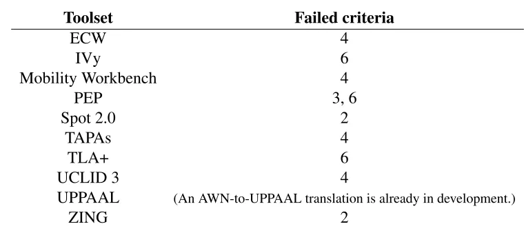
In the first stage of the research mCRL2 was chosen as the target model checking toolset for the translation from AWN. This was done by choosing several criteria that the target toolset should satisfy. These criteria were used to make a selection of model checking toolsets found in internet databases [12] [13] [14]. In general, this selection process has suffered from a time constraint that was self-imposed to prevent the comparison of existing toolsets from being taken further than what is beneficial to this graduation project. Searching for unambiguous information about a certain model checking toolset was therefore stopped after approximately 1.5 hours. As a consequence, information might have been missed, and a toolset might have been dismissed unjustly.

Furthermore, there are multiple model checking toolsets that are based on their own particular algebra or logic. A comparison of these toolsets would require much more in-depth study of and experience with these toolsets, which would consume valuable project time. It is therefore possible that relevant information was misunderstood or incorrectly considered to be ambiguous.

Toolset Failed criteria

ECW 4

IVy 6

Mobility Workbench 4

PEP 3, 6

Spot 2.0 2

TAPAs 4

TLA+ 6

UCLID 3 4

UPPAAL (An AWN-to-UPPAAL translation is already in development.)

ZING 2

Table 1.1: Toolsets that were rejected and why.

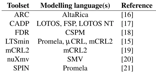
The chosen criteria for the model checking toolset to be targeted by the translation from AWN are these:

1. A toolset should have clear support for generic model checking, and not be specifically aimed at, for instance, code verification or probabilistic model checking.

2. A toolset should have accessible, complete, and up-to-date formal semantics. This is required to prove the validity of the translation later in the research.

3. A toolset should have sufficient online documentation, including examples, tutorials, and possibly active user forums. This makes the toolset easier to learn, which facilitates more advanced use of that toolset as a back end for AWN.

4. A toolset must have been updated since 2012 (in the previous 5 years). This criteria aims to exclude tools that are no longer being developed and improved without having to rely on that information being publicly available (which it may not be), and to exclude tools with very slow release cycles.

5. A toolset should have a text-based, sufficiently expressive modeling language, so that the result of a translation is easily readable by users and manual adjustments can be made if desired. This implies the presence of a framework for modeling concurrent systems, for example, but also more basic features, such as data types, functions, arithmetical operators, and so on. 6. A toolset should have a sufficiently expressive property language, so that a maximum number

of different types of properties of a protocol can be analyzed. Toolsets with more expressive property languages are preferred over those with less expressive ones.

Toolset Modelling language(s) Reference

ARC AltaRica [16]

CADP LOTOS, FSP, LOTOS NT [17]

FDR CSPM [18]

LTSmin Promela,µCRL, mCRL2 [15]

mCRL2 mCRL2 [19]

nuXmv SMV [20]

SPIN Promela [21]

Table 1.2: Selected toolsets.

2

Why MDE?

The translation from AWN to mCRL2 has been implemented using model-driven engineering techniques. This means that rather than object-focused, the implementation is model-focused, where ‘models’ are essentially groups of related classes.

Model-driven engineering (MDE) has been chosen because they provide tools to construct new models from existing models viatransformations. This means that if an AWN specification is stored in an input model and an mCRL2 specification can be stored in an mCRL2 model, a transformation can be created that goes from the former to the latter – the transformation being the implementation of the AWN-to-mCRL2 translation, of course. In short, the basic MDE architecture precisely matches the structure needed by a translation framework for AWN.

Models conform to the structure defined by metamodels, which conform to ametametamodel. Frameworks can be built around such a metametamodel so that software can be generated that accepts models conforming to a customized metamodel as input. Transformation languages such as ATL and QVTO are such frameworks. Xtext is a framework that can be used to generate the core of an Eclipse plug-in, which means that it is easy to create an editor with the features expected by average users.

Another advantage of MDE is that it automatically sets a high standard for the degree at which the different aspects of an implementation are separated, similar toaspect-oriented techniques[22]. Other approaches in software engineering are often more prone to situations in which multiple concerns are addressed in one place, reducing code maintainability.

The disadvantage of the MDE approach is that it requires developers to know 1 general-purpose language (Java or another language supported by MDE tools) and at least 4 DSLs (there exist different DSLs for the same purpose in MDE) instead of only 1 language:

• One for specifying the AWN metamodel, and potentially the mCRL2 metamodel;

• One for specifying the grammar of the AWN input language;

• One for specifying the transformation from AWN to mCRL2;

2. Formal translation

_{2. Formal translation}

1

AWN semantics

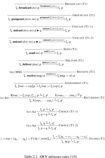
This first section will give an overview of the semantics of AWN. The corresponding inference rules can be found in Tables 2.1 to 2.5. The labels that identify the inference rules show a number in between brackets which refers to the table in [6] from which they were copied. For a full description of the semantics of AWN, consult that document.

The semantics of AWN are divided into four ‘levels’:

• Thesequential process level. The semantics of this level describe how the decision flow of a single process of a protocol is specified, including guards, variable assignments, and local broadcasts.

• Theparallel process levelcombines multiple sequential processes into a single parallel process so that they can run on the same node. Combined sequential processes can only communicate in one direction.

• Thenode levelgives parallel processes their address and the set of addresses of nodes that are within their transmission range. It also adds network behavior such as connecting and disconnecting to parallel processes.

• Thenetwork leveldetermines which behavior is ultimately allowed to occur: a node that tries to transmit a message, for example, will only succeed if a recipient actively cooperates.

1.1 Sequential process level

The decision flow of a protocol is determined by a composition of sequential processes. Sequential processes have a signatureX(var1, . . . ,varn)consisting of a nameX and a number of parameters

grammar:

SP ::= [φ]SP | _Jvar:=exp_KSP

| broadcast(msg).SP | groupcast(dests,msg).SP

| unicast(dest,msg).SP_ISP | send(msg).SP

| deliver(data).SP | receive(msg).SP

| X(exp₁, . . . ,exp_n)

Clearly, sequential processes have many possibilities to determine the behavior of a protocol: using guards[φ]SP, they can elect to perform certain actions only under particular circumstances; variable assignment_Jvar:=exp_KSP allows the contents of the internal data structure of the sequential process to be changed; they can perform abroadcast,groupcast,unicast,send,deliver, orreceiveaction, which allow processes to exchange messages in specific ways; they can let another sequential process

X(exp₁, . . . ,exp_n)determine their subsequent behavior; and they can choose non-deterministically

between multiple of these possibilities via the+operator.

The different types of message exchanges have distinct purposes: broadcast is used to send a message toallnodes in the network that are within range;groupcastdoes the same as long as nodes are in a specified subset;unicastallows a message to be sent to a specified node, continuing with its first branch p if that node is within range or continuing with a¬unicastaction and its second branch q if the transmission failed; andsendpasses a message to another sequential process running on the same node (see Section 1.2).

The receive action performs the complementary action: it intercepts a message (regardless of whether it originated from a broadcast, groupcast, unicast, or send action) and stores it in a specified variable. Messages (or rather, the relevant data that they contain) can exit the network via thedeliveraction.

Inference rules BROADCAST(T1) to GUARD (T1) in Table 2.1 give the semantics of sequential

process expressionsξ,pin AWN. In these expressions,ξ is a variable-to-value mapping andpthe current sequential process expression. Note that inference rules that contain expressions of the form ξ(exp)are only defined ifexpis bound byξ!

Interpretation of guards

Guards in AWN use the syntax[φ]p. The rule in the original semantics of AWN that allows guards to be constructed makes use of the notationξ −→φ ζ [6]. Informally, this syntax is defined to mean that the variable-to-value mappingζ extends variable-to-value mappingξ with new mappings for variables unmapped inξ in such a way thatφ underζ evaluates totrue. This allows AWN to set variables in guards using a type ofpattern matching.

For example, letipanddatabe unmapped when the following expression is executed:

receive(msg).[msg=Message(ip,data)] p

The execution will reach pif and only if a message is received that conforms to the structure

BROADCAST(T1)

ξ,broadcast(ms).p−−−−−−−−−−→broadcast(ξ(ms)) ξ,p

GROUPCAST(T1)

ξ,groupcast(dests,ms).p−−−−−−−−−−−−−−−→groupcast(ξ(dests),ξ(ms)) ξ,p

UNICAST(T1-1)

ξ,unicast(dest,ms).p_Iq−unicast−−−−−−−−−−−−(ξ(dest),ξ(ms→)) ξ,p

UNICAST(T1-2)

ξ,unicast(dest,ms).pIq

¬unicast(ξ(dest),ξ(ms))

−−−−−−−−−−−−−→ξ,q

SEND(T1)

ξ,send(ms).p−−−−−−−→send(ξ(ms)) ξ,p

DELIVER(T1)

ξ,deliver(data).p−−−−−−−−−→deliver(ξ(data)) ξ,p

∀m∈MSG RECEIVE(T1)

ξ,receive(msg).p−−−−−−→receive(m) ξ[msg:=m],p

ASSIGNMENT(T1)

ξ,Jvar:=expKp

τ −

→ξ[var:=ξ(exp)],p

/0[var_i:=ξ(exp_i)]n i=1,p

a −

→ζ,p0 X(var₁,· · ·,var_n)def=p

∀a∈Act RECURSION(T1)

ξ,X(exp₁,· · ·,exp_n)−→a ζ,p0

ξ,p−→a ζ,p0

∀a∈Act CHOICE(T1-1)

ξ,p+q−→a ζ,p0

ξ,q−→a ζ,q0

∀a∈Act CHOICE(T1-2)

ξ,p+q−→a ζ,q0

ζ=ξ[q₁:=e1,· · ·,qn:=en]

ζ(φ) =true∧ {q₁,· · ·,q_n}=FV(φ)\DOM(ξ) GUARD(T1)

ξ,[φ]p−→τ ζ,p

For the correctness proof of the translation, a formal interpretation ofξ −→φ ζ is needed. To this end, GUARD(T1) uses the following side condition:

ζ(φ) =true∧ {q₁,· · ·,q_n}=FV(φ)\DOM(ξ)

where FV(φ)are the free variables inφ andDOM(ξ) ={x|x:=y∈ξ }.

P−→a P0

∀a6=receive(m) PARALLEL(T2-1) PhhQ−→a P0hhQ

Q→−a Q0

∀a6=send(m) PARALLEL(T2-2) PhhQ→−a PhhQ0

P−−−−−−→receive(m) P0 Q−−−−→send(m) Q0

∀m∈MSG PARALLEL(T2-3)

PhhQ−→τ P0hhQ0

Table 2.2: AWN inference rules (2/5)

1.2 Parallel process level

Sequential processes are combined into a single parallel process according to the following grammar: PP ::= ξ,SP | PPhhPP

The sequential processes form a pipeline for messages: processes can use thesendaction to send a message to the process to their left, where thereceiveaction can be used to receive it. Only the rightmost sequential process can usereceiveto listen for messages from other nodes in the network. See inference rules PARALLEL(T2-1) to PARALLEL(T2-3) in Table 2.2 for the semantics.

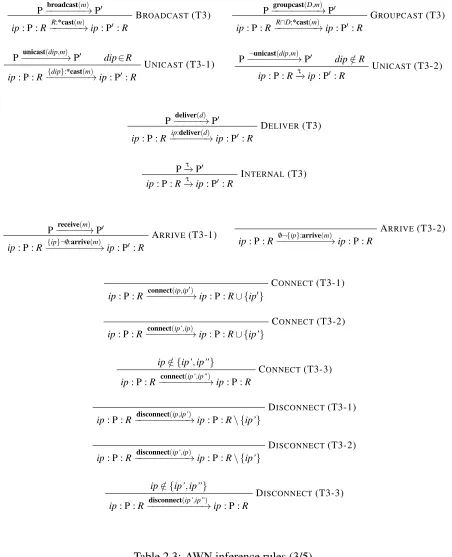
1.3 Node level

The rules for the node level, BROADCAST(T3) to DISCONNECT(T3-3), can be found in Table 2.3. These rules add network behavior to parallel processes: they allow them to connect, to disconnect, to deliver data objects, and they rewrite actions such asbroadcast(m)andunicast(d,m)in terms of the current state of the network: broadcast(m) will be converted toR:starcast(m), whereR

is the set of addresses of all nodes within range, whereasunicast(d,m)is converted to the action

{d}:starcast(m)because only the node with addressdshould be a recipient.

P−−−−−−−→broadcast(m) P0 _B

ROADCAST(T3) ip: P :R−−−−−−→R:*cast(m) ip: P0:R

P−−−−−−−−−→groupcast(D,m) P0 _G

ROUPCAST(T3) ip: P :R−−−−−−−−→R∩D:*cast(m) ip: P0:R

P−−−−−−−−→unicast(dip,m) P0 dip∈R

UNICAST(T3-1) ip: P :R−−−−−−−−→{dip}:*cast(m) ip: P0:R

P−−−−−−−−−→¬unicast(dip,m) P0 dip∈/R

UNICAST(T3-2) ip: P :R−→τ ip: P0:R

P−−−−−→deliver(d) P0 _D

ELIVER(T3) ip: P :R−−−−−−−→ip:deliver(d) ip: P0:R

P−→τ P0 _I

NTERNAL(T3) ip: P :R−→τ ip: P0:R

P−−−−−−→receive(m) P0 _A

RRIVE(T3-1) ip: P :R−−−−−−−−−→{ip}¬/0:arrive(m) ip: P0:R

ARRIVE(T3-2) ip: P :R−−−−−−−−−→/0¬{ip}:arrive(m) ip: P :R

CONNECT(T3-1) ip: P :R connect(ip,ip

0₎

−−−−−−−−→ip: P :R∪ {ip0}

CONNECT(T3-2) ip: P :R−−−−−−−−→connect(ip’,ip) ip: P :R∪ {ip’}

ip∈ {/ ip’,ip”}

CONNECT(T3-3) ip: P :R−−−−−−−−−→connect(ip’,ip”) ip: P :R

DISCONNECT(T3-1) ip: P :R−−−−−−−−−−→disconnect(ip,ip’) ip: P :R\ {ip’}

DISCONNECT(T3-2) ip: P :R−−−−−−−−−−→disconnect(ip’,ip) ip: P :R\ {ip’}

ip∈ {/ ip’,ip”}

DISCONNECT(T3-3) ip: P :R−−−−−−−−−−→disconnect(ip’,ip”) ip: P :R

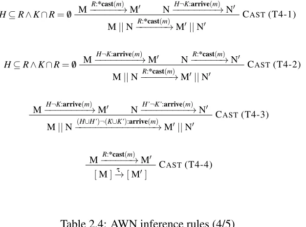
1.4 Network level

A partial network is constructed through parallel composition of nodes (via the||operator): M ::= ip: PP :R | M||M

Parallel nodes canexchange messagesaccording to rules CAST(T4-1) to CAST(T4-4) in Table 2.4. These exchanges occur through synchronization ofR:starcast(m)andH¬K:arrive(m)actions (where¬is simply a syntactic separator of the setsH andK). Of these two actions,H¬K:arrive(m) is where a messagemarrives at the nodes in the setHand wheremis ignored by the nodes in the set

K(because they are out of range). It is necessary for synchronization thatH⊆Rand thatK∩R= /0 becauseRinR:starcast(m)is the set of addresses of the intended recipients within range.

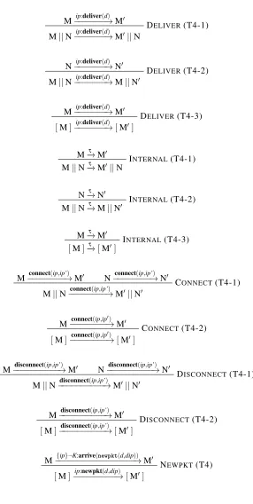
Encapsulation ([_]) allows a partial network M to be converted into a complete network [M]. Encapsulation also restricts the set of actions exposed by a network to τ, connect(ip,ip’) and

disconnect(ip,ip’),ip:newpkt(data,d), andip:deliver(data).

These actions have the following meanings. As usual in process algebra, τ is an action that is hidden from the environment of the network. Actionsconnect(ip,ip’)and disconnect(ip,ip’) represent events within the network where a node with addressip’respectively enters or leaves the range of a node with addressip(note that all nodes must agree on this topology change). Action

ip:newpkt(data,d)is the event where a data objectdto be delivered at the node with address d

is injected into the network (wrapped into a messagenewpkt(data,d)) at the node with addressip, whereas actionip:deliver(data)is the actual delivery of a data object at the node with addressip. The accompanying inference rules are DELIVER (T4-1) to NEWPKT(T4) in Table 2.5.

M−−−−−−→R:*cast(m) M0 N−−−−−−−−→H¬K:arrive(m) N0

H⊆R∧K∩R=/0 CAST(T4-1)

M||N−−−−−−→R:*cast(m) M0||N0

M−−−−−−−−→H¬K:arrive(m) M0 N−−−−−−→R:*cast(m) N0

H⊆R∧K∩R=/0 CAST(T4-2)

M||N−−−−−−→R:*cast(m) M0||N0

M−−−−−−−−→H¬K:arrive(m) M0 N−−−−−−−−−→H’¬K’:arrive(m) N0

CAST(T4-3) M||N−−−−−−−−−−−−−−−→(H∪H’)¬(K∪K’):arrive(m) M0||N0

M−−−−−−→R:*cast(m) M0 _C

AST(T4-4)

[M]−→τ [M0]

M−−−−−−−→ip:deliver(d) M0 _D

ELIVER(T4-1) M||N−−−−−−−→ip:deliver(d) M0||N

N−−−−−−−→ip:deliver(d) N0 _D

ELIVER(T4-2) M||N−−−−−−−→ip:deliver(d) M||N0

M−−−−−−−→ip:deliver(d) M0 _D

ELIVER(T4-3)

[M]−−−−−−−→ip:deliver(d) [M0]

M−→τ M0 _I

NTERNAL(T4-1) M||N−→τ M0||N

N−→τ N0 _I

NTERNAL(T4-2) M||N−→τ M||N0

M−→τ M0 _I

NTERNAL(T4-3)

[M]−→τ [M0]

M−−−−−−−−→connect(ip,ip’) M0 N−−−−−−−−→connect(ip,ip’) N0

CONNECT(T4-1) M||N−−−−−−−−→connect(ip,ip’) M0||N0

M connect(ip,ip 0₎

−−−−−−−−→M0 _C

ONNECT(T4-2)

[M] connect(ip,ip

0₎

−−−−−−−−→[M0]

M−−−−−−−−−−→disconnect(ip,ip’) M0 N−−−−−−−−−−→disconnect(ip,ip’) N0 _D

ISCONNECT(T4-1) M||N−−−−−−−−−−→disconnect(ip,ip’) M0||N0

M−−−−−−−−−−→disconnect(ip,ip’) M0 _D

ISCONNECT(T4-2)

[M]−−−−−−−−−−→disconnect(ip,ip’) [M0]

M−{−−−−−−−−−−−−−−−−ip}¬K:arrive(newpkt(d,dip→)) M0 _N

EWPKT(T4)

[M]−−−−−−−−−→ip:newpkt(d,dip) [M0]

1.5 AWN examples

Listings 2.1 to 2.4 contain simple examples to illustrate how AWN might be used. The example of Listing 2.1 defines a radio tower (RadioTower, line 1) that broadcasts messages to radios (Radio, line 4) within range. Each message contains a value 1 higher than the value of the preceding message, and radios store the most recently received message. A specific network related to this example might be defined as in lines 6 through 9: the radio tower has address 1, there are 3 radios with addresses 2 to 4, and only radios with addresses 2 and 4 are within range of the radio tower.

1 RadioTower(msgVal: Integer) =

2 broadcast(new Message(msgVal)) . RadioTower(msgVal + 1);

3

4 Radio(lastMsg: Message) = receive(msg) . Radio(msg); 5

6 RadioNetwork = [ 1 : RadioTower(1) : { 2, 4 } ||

7 2 : Radio(null) : { 1 } ||

8 3 : Radio(null) : /0 ||

9 4 : Radio(null) : { 2 } ];

Listing 2.1: AWN radio tower example.

1 ChatClient(lastMsg: Message, sentMsg: Boolean) =

2 receive(msg) . ChatClient(msg, sentMsg)

3 + unicast(1, Message("Hello everyone!")) .

4 ChatClient(lastMsg, true) I ChatClient(lastMsg, false);

5

6 ChatServer() = receive(msg) . broadcast(msg) . ChatServer();

Listing 2.2: AWN ‘chat client’ example.

The second example introduces a ‘chat client’ (ChatClient, line 1) that listens for messages similar to theRadioprocess. However, the server (ChatServer, line 6) only forwards messages that it receives from clients within range. These messages are non-deterministically sent by clients to a node within range that has address 1, which is assumed to be the chat server. Clients always send the same message.

Listing 2.3 defines a simple flooding protocol. Each node of a network runs the same process (Flood), line 1). This process injects its message into the network at a non-deterministic time (similar toChatClientfrom the previous example, but now nodes send their message a maximum of one time). The process also listens for incoming messages: for each node address, it stores the contents of the first message received from that node.

1 Flood(msgSent: Boolean, store: IP 7→ Text) =

2 receive(msg) . [msg = Message(ip', text)] (

3 [ip' 7→ text ∈ store] . Flood(msgSent, store)

4 + [ip' 7→ text ∈/ store] .

5 J store := store[ip' 7→ text] K

6 broadcast(msg) . Flood(msgSent, store))

7 + [¬ msgSent] broadcast(new Message("Hello everyone!")) .

8 Flood(true, store);

Listing 2.3: AWN flooding example.

1 Queue(queue: Sequence(Message)) =

2 receive(msg) . Queue(queue→append(msg))

3 + [queue→size() > 0] (

4 receive(msg) . Queue(queue→append(msg))

5 + send(queue→at(0)) . Queue(queue→remove(0))

6 );

7

8 FloodWithQueue = Flood(false, /0) << Queue(/0); 9

10 FloodNetwork = [ 1 : FloodWithQueue() : { 2, 3, 4 } ||

11 2 : FloodWithQueue() : { 1, 3 } ||

12 3 : FloodWithQueue() : { 1, 2 } ||

13 4 : FloodWithQueue() : { 1 } ];

Listing 2.4: AWN queued flooding example.

2

mCRL2 semantics

For the translation from AWN to mCRL2, the features of mCRL2 related to time will not be used. This section will therefore give theuntimedfragment of the semantics of mCRL2 (a similar approach as the one used in [23]). Note that only an overview is provided here; refer to the book in which mCRL2 is documented [24] for the full semantics.

2.1 Grammar

Similar to sequential processes in AWN, mCRL2 processes have a signatureX(var1:D1,· · ·,varn:

D_n)whereX is a name andvari are process parameters of data typeDi. All mCRL2 processes are contained within the set PD. The behavior of mCRL2 processes is specified by expressions conforming to the following grammar:

p ::= δ | ω | p.p | p+p | c→p | c→pp | ∑_x:Dp

| p||p | ΓC(p) | ∇V(p) | ∂B(p) | ρR(p) | τI(p)

| X(d1,· · ·,dn)

ω ::= τ | a(d1,· · ·,dn) | ω|ω

In this grammar,δ represents a deadlocked process, meaning that it cannot make any transitions. To do an actionω, one only has to write it; however, mCRL2 actually usesmulti-actions, which are actions that potentially consist of multiple action labelsathat can each carry their own data. The actionτis the empty multi-action with the property thatω|τ=τ|ω =ω.

Processes can be chained, or choices can be made between them, either by checking a conditionc

or non-deterministically – the expression∑_x:Dp, in particular, is used to express a non-deterministic

choice between summands for every possible value ofx, a variable of data type D. Expressions p and q can be put in parallel by writing p||q. FinallyΓC,∇V,∂B,ρR, andτI are operators that can influence the behavior of a process in various ways – their descriptions can be found in 2.3.

2.2 Inference rules

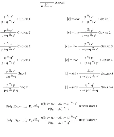
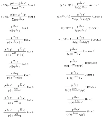
Tables 2.6 and 2.7 list rules in Plotkin style [25] for the structural operational semantics of mCRL2 process expressions. In these rules, several notations are used that require short explanations:

• The_X-predicate is used to indicate the mCRL2 termination state – a process ‘goes here’ when it has no more actions to do;

• The syntaxd: D means that variabledis of type D;

• MDrefers to the set of all possible semantic values of type D. Furthermore, ife∈MDthen

there existst_e, a syntactic symbol foresuch that_Jt_eK=e(see Definition 15.2.17 in [24]);

• ω denotes a multi-action from which all data has been removed;

AXIOM

α−−→JαK X

p−→ω _X

CHOICE1 p+q−→ω _X

p−→ω p0

CHOICE2 p+q−→ω p0

q−→ω _X

CHOICE3 p+q−→ω _X

q−→ω q0

CHOICE4 p+q−→ω q0

p−→ω _X

SEQ1 p.q−→ω q

p−→ω p0

SEQ2 p.q−→ω p0.q

p−→ω _X

JcK=true GUARD1

c→p−→ω _X

p−→ω p0

JcK=true GUARD2

c→p−→ω p0 p−→ω _X

JcK=true GUARD3

c→pq−→ω _X

p−→ω p0

JcK=true GUARD4

c→pq−→ω p0 q−→ω _X

JcK=false GUARD5

c→pq−→ω _X

q−→ω q0

JcK=false GUARD6

c→pq−→ω q0

q[d1:=t1,· · ·,dn:=tn] ω −→_X

P(d1: D1,· · ·,dn: Dn)

def

=q RECURSION1

P(t1,· · ·,tn) ω −→_X

q[d1:=t1,· · ·,dn:=tn] ω −→q0 P(d1: D1,· · ·,dn: Dn)

def

=q RECURSION2

P(t1,· · ·,tn) ω −→q0

p[d:=te] ω −→_X

e∈MD SUM1

∑_d:Dp

ω −→X

p[d:=te] ω −→p0

e∈MD SUM2

∑d:Dp−→ω p0 p−→ω _X

PAR1 p||q−→ω q

p−→ω p0

PAR2 p||q−→ω p0||q p−→ω p0 q−→ω q0

PAR3 p||q−−→ω|ω p0||q0

q−→ω _X

PAR4 p||q−→ω p

q−→ω q0

PAR5 p||q−→ω p||q0 p−→ω _X q−→ω _X

PAR6 p||q−−→ω|ω _X

p−→ω p0 q−→ω _X

PAR7 p||q−−→ω|ω p0

p−→ω _X q−→ω q0 PAR8 p||q−−→ω|ω q0

p−→ω _X

ω∈V∪ {τ} ALLOW1

∇V(p) ω −→_X

p−→ω p0

ω∈V∪ {τ} ALLOW2

∇V(p) ω

−→∇V(p0)

p−→ω _X

ω{}∩B=/0 BLOCK1

∂B(p) ω −→_X

p−→ω p0

ω{}∩B=/0 BLOCK2

∂B(p)−→ω ∂B(p0)

p−→ω _X

RENAME1

ρR(p) R •ω −−→_X

p−→ω p0

RENAME2

ρR(p) R•ω −−→ρR(p0)

p−→ω _X

COMM1

ΓC(p) γC(ω)

−−−→_X

p−→ω p0

COMM2

ΓC(p) γC(ω) −−−→ΓC(p0)

p−→ω _X

HIDE1

τI(p) θI(ω)

−−−→_X

p−→ω p0

HIDE2

τI(p) θI(ω)

−−−→τI(p0)

Finally, the rules in Tables 2.6 and 2.7 make use of_Jω_K-brackets, which denote the semantic value ofω. mCRL2 provides rules for how to apply these brackets are applied to expressions; see Definition 2.1.

Definition 2.1 The following rules apply to_Jexp_K:

JτK=τ

Ja(t1,· · ·,tn)K=a(Jt1K,· · ·,JtnK) Jα|βK=JαK|JβK

These rules were obtained from Definition 15.2.12 of the book that documents mCRL2 [24].

2.3 Special operators

The∇V,∂B,ΓC,ρR, andτI are special operators that affect the actions that a process can perform. The following subsections describe these operators in greater detail.

Allow operator

The allow operator∇V only allowsτ and actions and multi-actions that are in the set of multi-actions

V from occurring in the operand. Its behavior follows ALLOW1 and ALLOW2 in Table 2.7.

Block operator

The block operator∂B(see BLOCK1 and BLOCK2) prevents actions that are inBfrom occurring in the operand (with the exception ofτ). Any (multi-)action sharing an action withBis blocked – the blocked actions are not ‘subtracted’ from their multi-actions!

Communication operator

The communication operatorΓC (see COMM 1 and COMM 2) modifies multi-actions that contain combinations of action labels by renaming those combinations to a specific action label. To this end, it requires a set of pairs(a1|. . .|an→b)wherea1|. . .|anis a multi-action without data andb an action label. This set is passed to an auxiliary functionγ, which is defined as follows:

γ/0(α) =α

γC1∪C2(α) =γC1(γC2(α))

γ{a1|...|an→b}(α) = 

 

 

b(d)|γC(α\(a1(d)|. . .|an(d)))

where the operators\andv– although likely intuitively understood – are defined as

τ\α =τ

α\τ=α

α\(β|γ) = (α\β)\γ

(α|a(d₁,· · ·,d_n))\a(d₁,· · ·,d_n) =α

(α|a(d₁,· · ·,d_n))\b(e₁,· · ·,e_n) = (α\b(e₁,· · ·,e_n))|a(d₁,· · ·,d_n)

ifa6=b∨d1=6 e1∨ · · · ∨dn6=en and

τvα =true

a(d₁,· · ·,d_n)vτ=false

α|a(d1,· · ·,dn)vβ|a(d1,· · ·,dn) =α vβ

α|a(d1,· · ·,dn)vβ|b(e1,· · ·,en) = (α\b(e1,· · ·,en))|a(d1,· · ·,dn)vβ ifa6=b∨d₁=6 e₁∨ · · · ∨d_n6=e_n

respectively.

Rename operator

The rename operatorρR renames all actions in the operand with the nameatobfor alla→b∈R (wherea6=τ,b6=τ). To this end, the following auxiliary function is used in Table 2.7:

ρR(τ) =τ

ρR(a(d1,· · ·,dn)) =b(d1,· · ·,dn)ifa→b∈Rfor someb ρR(a(d1,· · ·,dn)) =a(d1,· · ·,dn)ifa→b∈/Rfor allb

ρR(α|β) =ρR(α)|ρR(β)

hide operator

The hide operatorτI replaces all actions in the operand with the nameabyτ for alla∈I. Due to the property thatω|τ=τ|ω=ω, theais simply removed instead ifais part of a multi-action.

The BLOCK1 and BLOCK2 inference rules in Table 2.7 describe the behavior of the hide operator

by using a functionθ. This function is defined as follows:

θI(τ) =τ

θI(a(d1,· · ·,dn)) =τ ifa∈I

2.4 mCRL2 data language

This section gives some details of how the data expression language of mCRL2 works.

Sort declarations

Types are called ‘sorts’ in mCRL2. There are predefined sorts, such asBool(boolean) andNat (natural numbers), but also custom sorts, which must be declared. With regard to this project,

structured sortsare particularly relevant.

Structured sorts are declared as a list of constructors with arguments. Consider the following grammar:

sort ::= sortsortName = structSort | · · ·

structSort ::= structstructSortConstructor1 | · · · | structSortConstructorn

structSortConstructor ::= constructorName(argName₁:argSort₁,· · ·,argName_n:argSort_n)

For example, the following code snippet declares a binary tree:

1 sort

2 BinTree

3 = struct Leaf | Node(value: Nat, leftChild: BinTree, rightChild: BinTree);

In order to create an instance of a structured sort, simply write one of the constructor with the appropriate number of parameter values, each of a compatible sort. Below, a binary tree with 3 nodes is defined:

1 Node(1, Node(2, Leaf, Leaf), Node(3, Leaf, Leaf))

To obtain the value of one of the arguments of a specific instance, use the name of the argument as a ‘getter’ function:

1 value(Node(9, Leaf, Leaf))

The data expression in the example above yields9.

Mappings and equations

mCRL2’s data language is a functional language. Functions in mCRL2 are defined through a

mappingand a number ofequations. The mapping specifies the function sort of the function, and the equations specify how the function should be evaluated.

The following code snippet defines a function that changes the value in aBinTreeto another value:

1 map

2 updateNodeValues: BinTree # Nat # Nat -> BinTree;

3 eqn

4 updateNodeValues(Leaf, i, j)

5 = Leaf;

6 updateNodeValues(Node(i, left, right), i, j)

7 = Node(j, updateNodeValues(left, i, j), updateNodeValues(right, i, j)); 8 updateNodeValues(Node(v, left, right), i, j)

The mapping specifies that the function takes aBinTreeand two natural numbers as input and produces a BinTreeas output. Three equations define a standard recursive algorithm: the first equation is the base case of the recursion; the second equation changes the value of the current node fromitojand then continues with the child nodes; and the third equation does the same but maintains the value of the current node.

2.5 mCRL2 examples

Listings 2.5 to 2.7 give an example of a system specification in mCRL2. Listing 2.5 first specifies some of the required actions in the actblock (lines 1 to 3). It then defines the two subsystems that constitute the television system as two separate processes: theVolumesubsystem (lines 6 to 8) allows the volume of the television to be turned up or down within the range 0 to 50, and the Channelsubsystem (lines 10 to 12) allows the channel (0 to 99) of the television to be changed by twice pressing a 0 to 9 button. The two subsystems can be easily composed using parallel composition (line 14). Theinitsection specifies the first state of the entire television system.

1 act

2 volume_down, volume_up;

3 press: Integer;

4 5 proc

6 Volume(volume: Integer) =

7 volume_down . Volume(if(volume > 0, volume - 1, 0)) 8 + volume_up . Volume(if(volume < 50, volume + 1, 50)); 9

10 Channel(channel: Integer) =

11 sum n1:{0..9} . press(n1) .

12 sum n2:{0..9} . press(n2) . Channel(n1 * 10 + n2);

13

14 Television = Channel(1) || Volume(25); 15

16 init

17 Television;

Listing 2.6 extends the television by adding a mute subsystem. This subsystem allows the user to turn the volume of the television on or off in its entirety by pressing the ‘mute’ button (line 6). The volume of the television is also turned back on when the user changes the volume of the television (line 7 and 8).

1 act

2 mute;

3 4 proc

5 Mute(muted: Boolean) =

6 mute . Mute(!muted)

7 + volume_down . Mute(false)

8 + volume_up . Mute(false); 9

10 Television2 = Channel(1) || Volume(25) || Mute(false);

Listing 2.6: Naive extension of the simple mCRL2 television example.

Naively, one might be tempted to add the new subsystem to the television by using another parallel composition as in line 10 of Listing 2.6. However, in that case thevolume_upandvolume_down actions of theVolumeandMutesubsystems would be independent, and it is therefore possible that the television model changes the volume without unmuting.

Instead, one should make use of the communication operatorΓand the block operator∂, which are discussed in subsections 2.3 and 2.3, respectively. Listing 2.7 shows how this can be accomplished: with the communication operator, thevolume_up and volume_down actions of theVolume and Mute subsystems are merged (and renamed to synced_volume_up and synced_volume_down, respectively) and then prevents any independent occurrences ofvolume_upandvolume_downwith the block operator.

1 act

2 synced_volume_down, synced_volume_up; 3

4 proc

5 Television3 = Channel(1) || ∂{volume_up,volume_down}

6 Γ{volume_up|volume_up→synced_volume_up,volume_down|volume_down→synced_volume_down}

7 (Volume(25) || Mute(false));

3

Translation function

The project was continued by designing atranslation functionfrom AWN to mCRL2. The function has been defined by a list oftranslation ruleswhich have been categorized according to one of two purposes, namely for translating AWN’s sequential process expressions or for translating higher-level process expressions of AWN. The translation rules for both purposes are discussed in the following sections.

3.1 Translating sequential process expressions

The rules for translating sequential process expressions can be found in Table 2.8.

TV(ξ,broadcast(ms).p) =∑D:T(Set(IP))cast(UIP,D,Tξ(ms)).TV(ξ,p)whereD∈/T(V) T1 TV(ξ,groupcast(dests,ms).p) =∑D:T(Set(IP))cast(Tξ(dests),D,Tξ(ms)).TV(ξ,p)whereD∈/T(V) T2

TV(ξ,unicast(dest,ms).pIq) =cast({T_ξ(dest)},{T_ξ(dest)},T_ξ(ms)).TV(ξ,p) +¬uni({T_ξ(dest)},/0,T_ξ(ms)).TV(ξ,q) T3 TV(ξ,send(Tξ(ms)).p) =send(/0,/0,Tξ(ms)).TV(ξ,p) T4

TV(ξ,deliver(data).p) =∑ip:T(IP)del(ip,Tξ(data)).TV(ξ,p)whereip∈/T(V) T5

TV(ξ,receive(msg).p) =∑_D,D':T(Set(IP)),T(msg):T(MSG)receive(D,D',T(msg)).TV∪{_msg}(ξ\msg,p)whereD,D'∈/T(V) T6

TV(ξ,Jvar:=expKp) =∑tmp:sort(T(var))(tmp=Tξ(exp))→∑T(var):sort(T(var))(T(var) =tmp)→ T7

t(/0,/0,msg_dummy).TV∪{var}(ξ\var,p)wheretmp∈/T(V)

TV(ξ,X(exp1,· · ·,expn)) =X(Tξ(exp1),· · ·,Tξ(expn)) T8

where T(X(var1,· · ·,varn)def=p) =X(T(var1): sort(T_ξ(exp₁)),· · ·,T(varn): sort(T_ξ(exp_n)))def=T{var1,···,varn}(/0,p)

TV(ξ,p+q) =TV(ξ,p) +TV(ξ,q) T9

TV(ξ,[φ]p) =∑T(FV(φ)\V)Tξ(φ)→t(/0,/0,msgdummy).TV∪FV(φ)(ξ,p) T10

T(X(var1,· · ·,varn)

def

=p) =X(T(var1): sort(T(var1)),· · ·,T(varn): sort(T(varn)))

def

=T{var1,···,varn}(/0,p) T11

Table 2.8: Rules for translating AWN’s sequential process expressions

The translation rules in Table 2.8 use TV(ξ,p)as the signature of the translation function, where p is the sequential process expression to be translated,ξ is avaluation(a mapping from some variables to semantic values), andV is a set of AWN variables (those that are assigned up to this point, to be precise). TV(ξ,p)is only defined ifDOM(ξ)∪FV(p)⊆V where FV(p)are the free variables in p. Occasionally, the bindings for a specific variablevis removed fromξ by writingξ\vwhich is defined asξ restricted toDOM(ξ)\ {v}.

ξ is carried around exclusively for the benefit of the T_ξ(exp) function, which translates data expressions. The definition ofT_ξ(exp)is relatively complex:

T_ξ(exp)=def T(exp)T(x):=t_U(y)x:=y∈ξ

particular semantic value Y, the same syntactic representationt_Y will always be selected, which holds throughout the translation); and where the function T(exp)translates a syntactic AWN data expressionexpto a syntactic mCRL2 data expression. In order to abstract from the translation of data expressions at least to some extend,T(exp)is not further defined but simply assumed to exist

with the following properties: (i) T(exp)is a total function;

(ii) T(exp)behaves in such a way that∀exp,ξ .ξ(exp)is defined⇒_JT_ξ(exp)_K=U(ξ(exp));

(iii) exp=v⇔T(exp) =v'wherevis an AWN variable andv'is an mCRL2 variable; (iv) ∀exp.FV(T(exp)) ={T(v)|v∈FV(exp)}; and

(v) T(var1) =T(var2)⇔var1=var2.

The following subsections will elaborate on each of the translation rules in Table 2.8.

RuleT1: Broadcast

TV(ξ,broadcast(ms).p) =∑_D:T(Set(IP))cast(UIP,D,Tξ(ms)).TV(ξ,p)whereD∈/T(V) T1

This rule defines how abroadcastaction is translated to mCRL2. The resultingcastaction has three parameters and is then immediately followed by the translation of p.

The first parameter of thecastaction is the set of addresses of nodes that are the intended recipients of the messagems. Since a broadcastaction always attempts to reach all nodes with range, the value of this parameter is the universe of all node addresses (UIP).

The second parameter is the set of actual recipients. The sequential process does not have direct access to which nodes are within range, however, and the value of this parameter is therefore unknown. This has been solved by adding∑_D:T(Set(IP)), the resulting mCRL2 expression produces a castaction forallpossible values – superfluous actions will be eliminated at a later stage. The side condition ofT1ensures thatDis fresh.

The third parameter is the message that is sent translated to an mCRL2 expression by means of the

T_ξ(exp)function.

RuleT2: Groupcast

TV(ξ,groupcast(dests,ms).p) =∑_D:T(Set(IP))cast(Tξ(dests),D,Tξ(ms)).TV(ξ,p)whereD∈/T(V) T2

This rule defines how agroupcastaction is translated to mCRL2. Just like for the translation of

broadcast, the resultingcastaction has three parameters and is then immediately followed by the translation of p. The second and third parameter are also translated the same as forbroadcast(with the side condition ofT2ensuring thatDis fresh), but the first parameter is not: rather thanU_IPthe set

RuleT3: Unicast

TV(ξ,unicast(dest,ms).pIq) =cast({T_ξ(dest)},{T_ξ(dest)},T_ξ(ms)).TV(ξ,p) +¬uni({Tξ(dest)},/0,Tξ(ms)).TV(ξ,q) T3

The translation of theunicastaction produces two possible outcomes: if the destination node is within range, acastaction can occur, sending messagemsto the destination specified by the user and continuing by executing p; and it the destination node isnotwithin range, a¬uniaction can occur, followed by the execution of q.

RuleT4: Send

TV(ξ,send(Tξ(ms)).p) =send(/0,/0,Tξ(ms)).TV(ξ,p) T4

The translation rule for thesendaction is the simplest of them all: it produces a single action by the same name and with three parameters. The first and second parameter of this action are simply initialized with an empty set of node addresses (these parameters are strictly necessary because the signature ofsendmust match the signature of thereceiveaction) and the third parameter carries the messagemsthat is sent.

RuleT5: Deliver

TV(ξ,deliver(data).p) =∑_ip:T(IP)del(ip,Tξ(data)).TV(ξ,p)whereip∈/T(V) T5

The deliver action allows the contents of messages (data) to ‘leave’ a network. Such an event involves two items of information in AWN: the data that is leaving the network, and the node where the data is leaving. Accordingly, the rule above produces adelaction with these two items as its parameters.

However, a sequential process is unaware of the node on which it is running. The chosen solution for this problem is that adelaction is produced for every possible node addressip– superfluous actions will be eliminated at a later stage. The side condition of the rule ensures that the variableip is fresh.

RuleT6: Receive

TV(ξ,receive(msg).p) =∑D,D':T(Set(IP)),T(msg):T(MSG)receive(D,D',T(msg)).TV∪{msg}(ξ\msg,p)whereD,D'∈/T(V) T6

When receiving a message, a node at the level of a sequential process expression is unaware of three things: the intended recipients of the message,D; the actual recipients of the message,D'; and the contents of the message. A sequential process therefore considers all possiblereceiveactions that could occur, and relies on the composition with other parts of the specification to eliminate the superfluous ones.

RuleT7: Assignment

TV(ξ,Jvar:=expKp) =∑tmp:sort(T(var))(tmp=Tξ(exp))→∑T(var):sort(T(var))(T(var) =tmp)→ T7

t(/0,/0,msg_dummy).TV∪{var}(ξ\var,p)wheretmp∈/T(V)

mCRL2 does not provide its own syntax for assignments other than when parameter values are assigned when a new process is instantiated. A more improvised solution is used here, namely one where a ∑-operator and a guard ensure that a specific variable matches the assigned value (see the innermost/rightmost ∑-operator). The assigned value is fixed beforehand by a similar construction (see the outermost/leftmost∑-operator) in order to allow the target variable to be used in the computation of the assigned value. The variable in which the assigned value is stored,tmp, is fresh as a result of the side condition of the rule.

One might wonder about the three placeholder parameters of thet, or indeed about the reason why

twas used rather thanτ in the first place. The answer to the first riddle is that actions thatdocarry three useful parameters will be renamed totat a later stage, and one of the requirements of mCRL2 for renaming an actionatobis that the action signatures ofaandbare identical. The answer to the second riddle is that the concurrent behavior of theτ action in mCRL2 does not match the behavior of theτ action in AWN, and that it is necessary to treatτ as a ‘regular’ action until the network level has been reached.

Finally, process p is translated. It receives the information that in addition to the variables inV the variablevaris assigned.varis removed fromξ so that a potential old value ofvarcannot be used in the translation of p.

RuleT8: Process recursion

Process ‘calls’ are simply translated by referencing the mCRL2 counterpart of the named AWN process that is being ‘called’ and providing it with the translation of each of the parameter values that were provided in AWN:

TV(ξ,X(exp1,· · ·,expn)) =X(Tξ(exp1),· · ·,Tξ(expn)) T8

where T(X(var1,· · ·,varn)

def

RuleT9: Choice

A choice between two branches in AWN is translated directly to a choice between two summands in mCRL2:

TV(ξ,p+q) =TV(ξ,p) +TV(ξ,q) T9

RuleT10: Guard

TV(ξ,[φ]p) =∑T(FV(φ)\V)Tξ(φ)→t(/0,/0,msgdummy).TV∪FV(φ)(ξ,p) T10

The exclusive purpose of carrying around the set of assigned variablesV is to determine which variables are assigned as part of a guard action: any variable that is free in the guard conditionφ andnotinV (and is therefore unassigned at the moment of execution) will be added as a quantifier to the∑-operator. Obviously, this means that the subsequent process p must find FV(φ)– all free variables inφ – in its index parameterV.

One might wonder about the three placeholder parameters of thet, or indeed about the reason why

twas used rather thanτ. The answers to these riddles are given in the description of translation rule

T7.

RuleT11: Process definition

T(X(var1,· · ·,varn)

def

=p) =X(T(var1): sort(T(var1)),· · ·,T(varn): sort(T(varn)))

def

=T{var1,···,varn}(/0,p) T11

3.2 Translating higher-level process expressions

The rules for translating sequential process expressions can be found in Table 2.9.

T(ξ,p) =TDOM(ξ)(ξ,p) T12

T(PhhQ) =∇VΓ{r|s→t}(ρ{receive→r}T(P)||ρ{send→s}T(Q)) T13

whereV={t,cast,¬uni,send,del,receive}

T(ip: P :R) =∇VΓC(T(P)||G(tU(ip),tU(R))) T14 whereV={t,starcast,arrive,deliver,connect,disconnect}

whereC={cast|cast→starcast,¬uni|¬uni→t,del|del→deliver,receive|receive→arrive}

where G(ip,R) =∑_D,D':T(Set(IP)),msg:T(MSG)(R∩D=D')→cast(D,D',msg).G(ip,R)

+∑d:T(IP),msg:T(MSG)(d∈/R)→ ¬uni({d},/0,msg).G(ip,R)

+∑_data:DATAdel(ip,data).G(ip,R)

+∑_D,D':T(Set(IP)),msg:T(MSG)(ip∈D')→receive(D,D',msg).G(ip,R)

+∑_D,D':T(Set(IP)),msg:T(MSG)(ip∈/D')→arrive(D,D',msg).G(ip,R)

+∑_ip':T(IP)connect(ip,ip').G(ip,R∪ {ip'})

+∑_ip':T(IP)connect(ip',ip).G(ip,R∪ {ip'})

+∑_ip',ip:T(IP)(ip∈ {/ ip',ip})→connect(ip',ip).G(ip,R)

+∑_ip':T(IP)disconnect(ip,ip').G(ip,R\ {ip'})

+∑ip':T(IP)disconnect(ip',ip).G(ip,R\ {ip'})

+∑_ip',ip:T(IP)(ip∈ {/ ip',ip})→disconnect(ip',ip).G(ip,R)

T(M||N) =ρR∇VΓ{arrive|arrive→a}ΓC(T(M)||T(N)) T15

whereR={a→arrive,c→connect,d→disconnect,s→starcast}

whereV={a,c,d,deliver,s,t}

whereC={starcast|arrive→s,connect|connect→c,disconnect|disconnect→d}

T([M]) =∇Vρ{starcast→t}ΓC(T(M)||H) T16

whereV={t,newpkt,deliver,connect,disconnect}

whereC={newpkt|arrive→newpkt}

where H=∑_ip:T(IP),data:T(DATA),dest:T(IP)newpkt({ip},{ip},newpkt(data,dest)).H

The translation rules in Table 2.9 use T(p)as the signature of the translation function, where p is the process expression to be translated. Clearly, T(p)no longer has theξ parameter (ξ,p in ruleT12

forms a single parameter, the state of a sequential process in AWN to be precise), and it does not carry a set of assigned variablesV anymore. At this level of the AWN specification, syntactic data expressions have disappeared.

The following subsections will elaborate on each of the translation rules in Table 2.9.

RuleT12: Sequential process

This rule allows the rules from Table 2.9 to make use of the rules in Table 2.8:

T(ξ,p) =TDOM(ξ)(ξ,p) T12

Note thatξ,p forms a single parameter – namely the state of a sequential process in AWN – and that this state is separated into its two components, the valuationξ and the process syntax p. Furthermore, the set of assigned variablesV is assigned with the domain of ξ (in the implementation, this is almost never of any consequence; when proving the correctness of T(p), however, this becomes a different story).

RuleT13: Parallel processes

T(PhhQ) =∇VΓ{r|s→t}(ρ{receive→r}T(P)||ρ{send→s}T(Q)) T13

whereV={t,cast,¬uni,send,del,receive}

Two AWN processes in parallel are translated by applying several mCRL2 operators in sequence: 1. It must be possible in the final mCRL2 operator to differentiate between thereceiveactions that occur in T(P)and those that occur in T(Q), as well as between thesendactions that occur in T(P)and those that occur in T(Q). Thereceiveactions of T(P)are therefore renamed tor

and thesendactions of T(Q)tos.

2. The resulting processes are put in parallel.

3. Occurrences ofr|saction labels are replaced by ataction label (this is whythas been given three parameters).

4. Only a specific selection of actions is allowed to occur. This blocks all mCRL2 multi-actions that are impossible in AWN (such ast|t). In addition, all remainingractions are blocked (from now on, T(P)can onlyreceivemessages if they arrive via T(Q), but T(Q) can still

RuleT14: Node

T(ip: P :R) =∇VΓC(T(P)||G(tU(ip),tU(R))) T14

whereV={t,starcast,arrive,deliver,connect,disconnect}

whereC={cast|cast→starcast,¬uni|¬uni→t,del|del→deliver,receive|receive→arrive}

where G(ip,R) =∑_D,D':T(Set(IP)),msg:T(MSG)(R∩D=D')→cast(D,D',msg).G(ip,R)

+∑_d:T(IP),msg:T(MSG)(d∈/R)→ ¬uni({d},/0,msg).G(ip,R)

+∑data:DATAdel(ip,data).G(ip,R)

+∑_D,D':T(Set(IP)),msg:T(MSG)(ip∈D')→receive(D,D',msg).G(ip,R)

+∑D,D':T(Set(IP)),msg:T(MSG)(ip∈/D')→arrive(D,D',msg).G(ip,R)

+∑_ip':T(IP)connect(ip,ip').G(ip,R∪ {ip'})

+∑ip':T(IP)connect(ip',ip).G(ip,R∪ {ip'})

+∑_ip',ip:T(IP)(ip∈ {/ ip',ip})→connect(ip',ip).G(ip,R)

+∑ip':T(IP)disconnect(ip,ip').G(ip,R\ {ip'})

+∑_ip':T(IP)disconnect(ip',ip).G(ip,R\ {ip'})

+∑ip',ip:T(IP)(ip∈ {/ ip',ip})→disconnect(ip',ip).G(ip,R)

This rule elevates processes to the network level by synchronizing them with a process G that provides the address of the node on which they run and the set of addresses of nodes that are within transmission range. Through this synchronization, the actions cast, ¬uni, del, andreceive of a process T(P)are forced to have certain parameter values, which eliminates many – but not all – of the superfluous mCRL2 actions that are impossible in AWN. G also adds independent node behavior, namelyarrive(which allows a node to synchronize the arrival of messages at other nodes with the rest of the network),connect, anddisconnectactions.

At the end, only single actions with certain labels are permitted to occur: multi-actions produced by putting T(P)and G in parallel are blocked, and so are leftovercast,cast,¬uni,¬uni,del,del,

receive, andreceiveactions.

RuleT15: Parallel nodes

T(M||N) =ρR∇VΓ{arrive|arrive→a}ΓC(T(M)||T(N)) T15

whereR={a→arrive,c→connect,d→disconnect,s→starcast}

whereV ={a,c,d,deliver,s,t}

whereC={starcast|arrive→s,connect|connect→c,disconnect|disconnect→d}

This rule produces a sequence of mCRL2 operators that restricts the behavior of T(M)||T(N)in such a way that any remaining action that can occur has a possible counterpart in AWN. In particular, the sequence of mCRL2 operators enforces that:

• One process doesstarcastactionandthe other process does a matchingarriveaction;

• Both processes do the sameconnect,disconnect, orarriveaction;

RuleT16: Network

T([M]) =∇Vρ{starcast→t}ΓC(T(M)||H) T16

whereV ={t,newpkt,deliver,connect,disconnect}

whereC={newpkt|arrive→newpkt}

where H=∑_ip:T(IP),data:T(DATA),dest:T(IP)newpkt({ip},{ip},newpkt(data,dest)).H

At the highest level of the AWN specification, it is possible to inject messages into the network via

newpktactions. In mCRL2, this behavior is enabled by translation ruleT16. Anewpktaction is

generated from a remainingarriveaction (which means that all nodes in the network are taking this action in parallel) that has exactly one node both as intended and as actual destination. In addition, the message parameter of the action is forced to have a specificnewpktformat.

The rule also renames remnant starcast actions to t and finally blocks multi-actions such as

connect|newpktas well as leftoverarriveandnewpktactions.

3.3 Totalness

This section shows that the translation function T is total.

Lemma 3.1 The translation function T as defined via the rules in Tables 2.8 and 2.9 istotal; that is, T(P)is defined for all valid AWN expressions P.

Proof. The proof is trivial, and therefore given informally.

First, there must exist a matching translation rule for each rule of the grammar of AWN. This is indeed the case.

Second, there must exist a matching translation rule for each input at recursive applications of T. Considering that recursive applications only receive process expressions from the original AWN process expression as input, such as porq, these process expressions must match the grammar of AWN, and therefore a matching translation rule must exist.

Third, there should be no infinite recursion. Since the input at recursive applications of T is always a strictly smaller expression than the input of the enveloping translation rule, recursion is always finite.

Finally,T_ξ(e)must be defined for all valid data expressionse. Combining property (i) of T_ξ(e) with the fact that∀e∈M_sort(e) .∃t._Jt_K=e(see Section 2.2) whereM_Dis the set of all semantic

3.4 Translation relation

Proving the correctness of the translation function involves showing the existence of a strong bisimulation between an AWN process and its translated counterpart in mCRL2. Because a strong bisimulation is a relation, it is useful to express the translation function as relation:

eT def

={(P,T(P))|P is an AWN parallel process, node, or (partial) network expression} (2.1)

Ultimately, however, the correctness proof will be a statement about the following relation:

eTτ

def

=([M],τ{t}T([M]))

[M]is an AWN network expression (2.2)

According to Lemma 3.1, both relations are defined for all valid AWN expressions of a matching type.

3.5 Action relation

The translation function T changes AWN actions to mCRL2 actions in a manner that is not always straightforward. To formally prove the correctness of T, the precise relation between AWN actions and mCRL2 actions must be made explicit first. The relation is calledA and its definition can be found in Table 2.10.

A def

={

({τ},{t(U(D),U(R),U(m))}), (2.3)

({broadcast(ξ(ms))},

cast(_JUIPK,D,JTξ(ms)K)

D∈T(Set(IP)) ), (2.4)

({groupcast(ξ(dests),ξ(ms))},cast(_JT_ξ(dests)_K,D,_JT_ξ(ms)_K)D∈T(Set(IP)) ), (2.5) ({unicast(ξ(dest),ξ(ms))},cast(JTξ({dest})K,JTξ({dest})K,JTξ(ms)K) ), (2.6) ({ ¬unicast(ξ(dest),ξ(ms))},¬uni(JTξ({dest})K,J/0K,JTξ(ms)K) ), (2.7) ({send(ξ(ms))},send(J/0K,J/0K,JTξ(ms)K) ), (2.8) ({deliver(ξ(data))},

del(î,_JTξ(data)K)

î∈T(IP) ), (2.9)

({receive(m)},

receive(D,D',U(m))D,D'∈T(Set(IP)) ), (2.10) ({R:*cast(m)},{starcast(U(D),U(R),U(m))}), (2.11)

({ip:deliver(d)},{deliver(U(ip),U(d))}), (2.12)

({H¬K:arrive(m)},

(

arrive(D,D',U(m))

D,D'∈T(Set(IP)) D'⊆D H⊆D' K∩D'=/0

)

), (2.13)

({connect(ip’,ip”)},{connect(U(ip’),U(ip”))}), (2.14)

({disconnect(ip’,ip”)},{disconnect(U(ip’),U(ip”))}), (2.15)

({ip:newpkt(d,dip)},{newpkt({U(ip)},{U(ip)},newpkt(U(d),U(dip)))}) (2.16)