Natural and formal infinities

University of Warwick institutional repository: http://go.warwick.ac.uk/wrap This paper is made available online in accordance with

publisher policies. Please scroll down to view the document itself. Please refer to the repository record for this item and our policy information available from the repository home page for further information.

To see the final version of this paper please visit the publisher’s website. Access to the published version may require a subscription.

Author(s): David Tall

Article Title: Natural and Formal Infinities Year of publication: 2001

Link to published version: http://dx.doi.org/ 10.1023/A:1016000710038 Publisher statement: The original publication is available at

Natural and Formal Infinities

David Tall

Mathematics Education Research Centre Institute of Education

University of Warwick Coventry CV4 7AL e-mail: David.Tall@warwick.ac.uk

Concepts of infinity usually arise by reflecting on finite experiences and imagining them extended to the infinite. This paper will refer to such personal conceptions as natural infinities. Research has shown that individuals’ natural conceptions of infinity are ‘labile and self-contradictory’ (Fischbein et al., 1979, p. 31). The formal approach to mathematics in the twentieth century attempted to rationalize these inconsistencies by selecting a finite list of specific properties (or axioms) from which the conception of a formal infinity is built by formal deduction. By beginning with different properties of finite numbers, such as counting, ordering or arithmetic, different formal systems may be developed. Counting and ordering lead to cardinal and ordinal number theory and the properties of arithmetic lead to ordered fields that may contain infinite and infinitesimal quantities. Cardinal and ordinal numbers can be added and multiplied but not divided or subtracted. The operations of cardinals are commutative, but the operations of ordinals are not. Meanwhile an ordered field has a full system of arithmetic in which the reciprocals of infinite elements are infinitesimals. Thus, while natural concepts of infinity may contain built-in contradictions, there are several different kinds of formal infinity, each with its own coherent properties, yet each system having properties that differ from the others.

The construction of both natural and formal infinities are products of human thought and so may be considered in terms of ‘embodied cognition’ (Lakoff and Nunez, 2000). The viewpoint forwarded here, however, is that formal deduction focuses as far as possible on formal logic in preference to perceptual imagery, developing a network of formal properties that do not depend on specific embodiments. Indeed, I shall show that formal theory can lead to structure theorems, whose formal properties may then be re-interpreted as a more subtle form of embodied imagery. Not only can natural embodied theory inspire theorems to be proved formally, but formal theory can also feed back into human embodiment, now subtly enhanced by the underlying network of formal relationships.

Introduction

After many centuries conceptualising various notions of infinity, and encountering puzzling conflicts, such as the Zeno paradoxes and logical difficulties of infinitesimals, matters came to a head at the end of the nineteenth century. Cantor (1895) developed a theory of infinite cardinals in which division was not possible, and he denied the theoretical existence of infinitesimals. Cantor’s theory, however, fell foul of the wrath of Kronecker who accused him of claiming that certain mathematical objects (such as cardinal infinity) existed without showing how they could be constructed. Kronecker’s view blossomed into the school of intuitionism led by Brouwer in the early twentieth century.

Two other major schools of thought grew at around the same time, each of which began approaches that encompassed formal definitions of infinite concepts. Hilbert (1900), in his celebrated address at the International Congress of Mathematicians, announced his list of the major problems for twentieth century mathematics. He also endorsed the formal approach to mathematics using the axiomatic method. This involves specifying a finite list of axioms to act as a foundation for a particular theory. He envisaged that such a strategy could lead to a total axiomatisation of mathematics, free from logical blemish. What mattered to him was not what concepts such as infinite cardinals are, but the consistency of the axiomatic theory that supports them. The third school of thought—the logicist approach led by Bertrand Russell, Gottlieb Frege and others—desired to define mathematical concepts purely in terms of logic1_.

All these theories encountered difficulties. The intuitionist school purposefully refused to use proof by contradiction, and this denied them a major tool used widely in twentieth century mathematics. Bertrand Russell found inconsistencies in aspects of Cantor’s set theory and suggested technical devices to overcome them. His pristine approach to logic was much admired, but pragmatic mathematicians carried on posing and solving research problems in ways that suited their problem context.

Hilbert’s formalist programme, therefore, cannot be completed in its entirety. In particular, any theory of infinite sets will include theorems that may be true but cannot be proved using only the techniques available in that system. Of course, one may add more axioms to the given theory (for instance, adding the axiom of choice to the limitations imposed by intuitionists). Such a tactic may prove a desired theorem, but the new axiom(s) allow the formulation of even more theorems that cannot be proved in the extended system. This is the Achilles’ heel of the formalist approach. Essentially an axiomatic system that attempts to talk about infinite structures has ‘too many’ properties to be able to prove them all by finite proofs using the available techniques.

This weakness did not destroy the desire to have an accepted axiomatic foundation for the many theories of modern mathematics. Mathematicians found that they can still prove a vast number of useful theorems in their axiomatic systems, even though some intractable problems may remain.

To explain ideas of infinity in a manner appropriate for a wide range of readers, the language used here will initially involve everyday colloquial meanings for a concept such as ‘set’, and whether that set is ‘finite’ or ‘infinite’. In everyday terms, a set is finite if we can – in principle – count it in the usual way, otherwise it is infinite. When mathematics is introduced to undergraduates, a formal concept – such as a ‘function’, ‘group’, ‘topological space’, ‘cardinal number’, ‘infinitesimal’, or whatever – is given in terms of a definition (or a list of axioms) in words and symbols, from which the properties of the given concept are deduced by mathematical proof.

be founded on a formal construction, complementing the more usual direction in which natural embodied conceptions are used to suggest axioms and proofs in a formal theory.

The cognitive construction of formal systems

The human mind is finite. By thinking about the possibility of performing a process again and again, we can easily reach out towards the potentially infinite. The counting sequence, 1, 2, 3, … is a potentially infinite collection. Given any whole number, there is a next one. The decimal notation allows us to represent whole numbers of arbitrarily large size. As a consequence, we humans can easily imagine a potential infinity as a process that goes on without end. But how do we think of the whole system in total, including all the numbers, all at one time? The answer is, of course, we don’t.

The human brain is not only finite, it copes with complexity by using a small conscious focus of attention, alighting on important information to assess a situation and take appropriate action. We therefore do not consciously focus on all the information at a given time, but move between different aspects, connected together mentally in a variety of ways.

For a given concept, we develop a whole concept image in the brain consisting of ‘the total cognitive structure that is associated with the concept, which includes all the mental pictures and associated properties and processes,’ (Tall & Vinner, 1981, p.152). This concept image grows and changes with experience and reflection. Such a biological entity cannot be totally coherent, for the various parts of the concept image develop at different times and in different ways; connections used on one occasion may be different from those evoked on another. Our concept images are full of partial experiences, focusing on a few aspects of a situation, linked together by various associations. What we attempt to do in mathematics is to rationalize the various experiences to build up as coherent an image as possible.

My colleague, Eddie Gray, observed James, aged six, in a group of children asked to type a sum with answer 8 into a graphic calculator. Whilst his friends typed in problems like 7+1, 4+4, 10–2, James typed:

How did he know that the answer to this problem is 8? He certainly did not do it by counting. James has sensed that there are patterns for the ‘next number’. After 9 comes 10, 11, 12, … after 19 comes 20, 21, 22, … after 99 comes 100, 101, 102, … after 999 comes 1000, …, and after 999,999 comes 1,000,000. He knows that 1,000 is ‘a thousand’ and 1,000,000 is ‘a million’ and he can type ‘a million’ into the calculator as 1000000. He has never counted a million. But his ideas of place value allow him to give it a meaning, and know that 999992+8 is ‘a million’ just as 2+8 is 10 and 992+8 is 1000. His brain does not contain ‘all the numbers’, but it does contain many sophisticated connections that give him strategies for giving meaning to any numbers that he cares to consider. It is from such a complex concept image that individuals attempt to build a shared system to be communicated in gestures, pictures, words and symbols, in ways that are mutually agreed to be appropriate.

Towards formal theories

For the young child, the construction of knowledge involves building on perceptions of the world using the growing sophistication of the concept image. The more sophisticated thinker notices properties of structures and relationships between them. Formal thinking begins when selected properties are isolated and used as concept definitions from which other properties may be deduced by mathematical proof. Pinto (1998), building on the natural/alien distinction of Duffin and Simpson (1993), identified two fundamentally different approaches to constructing axiomatic systems. A natural approach builds on concept imagery to give a personal meaning to the formal definition. This means constructing examples of the definition that are sufficiently generative to be used as a basis for thought experiments to imagine possible theorems and possible strategies for proving them. A formal approach, on the other hand, focuses essentially on the definitions, using formal deductions to build theorems in a manner that attempts to avoid any appeal to intuition. (Figure 1.)

mathematicians tend more towards a natural approach (particularly in subjects such as geometry and topology where mental pictures suggest theorems to be proved); others prefer an overall formal approach (for instance, in abstract symbolic theories). Nevertheless, it is a common goal to produce written formal proofs of theorems, whether constructed formally or underpinned by natural imagery.

axioms/definitions

Formal ideas

Examples/images CONCEPT

DEFINITION CONCEPT IMAGE

FORMAL DEDUCTIONS

proof: theorem: mental conception:

THOUGHT EXPERIMENTS

Natural experiences

Figure 1: Some constituents in constructing a formal theory

(Pinto, 1998; Pinto & Tall, 1999, 2001). However, many students failed to use the formal concept definition as a basis of deduction, instead preferring to build on their own personal version of the definition, sometimes inadequate, sometimes distorted, with the result that there was a broad spectrum of success and failure.

Before meeting axiomatic theories, the individual will already have some kind of informal (concept) image. Research shows that such concept images often persist long after

formal ideas are introduced (Fischbein et al., 1979). Personal informal images may involve essentially contradictory features. For instance, informal experiences invariably suggest that ‘the whole is greater than the part’, so that the whole set N of all natural numbers {1, 2, 3, …} is clearly greater than the part consisting of the set E of all even numbers {2, 4, 6, …}. Yet in the formal theory of cardinal numbers, two sets are defined to have ‘the same cardinal number’ if there is a one-to-one correspondence between them. The relation n´2n gives a one-to-one correspondence between N and E and so, in this case, the whole and the part have the same cardinal number.

Some natural learners find this experience alien and reject the theory of cardinal numbers, as did Kronecker in the early history of the subject. Some keep the informal ideas in a separate compartment, a strategy common to those formal learners who focus only on the formal theory without any desire to link it to informal knowledge. However, a powerful way forward for both natural and formal thinkers is to attempt to reconstruct their knowledge to resolve the conflict between old experiences and new evidence. For instance, the old experience that ‘the whole is greater than the part’ is still true for finite sets. The new evidence that this is false for the natural numbers may be turned to advantage; in a formal theory, we can define a set to be ‘infinite’ if and only if it can be put in one-to-one correspondence with a proper subset.

Who does not always use along with the double inequality a > b > c the picture of three points following one another on a straight line as the geometrical picture of the idea ‘between’? (Hilbert, 1902, p.442)

In this sense, embodied meanings are at the root of mathematics. However, a formal system may have more than one particular embodiment. In a formal system, only a small number of explicit properties are selected as the basis for deduction. Any deductions that are made, depending only on these initial axioms, must also apply to any other situation where the axioms happen to be satisfied. If a system satisfies the axioms of a vector space, it does not matter what the elements of the system are. They could be vectors in a plane, in n-dimensional space, solutions to a system of differential equations, a particular collection of functions. All that matters is that the structure involved satisfies the axioms for a vector space, with the immediate implication that it also satisfies all the properties deduced from the definition of a vector space.

Fully formal expositions of a mathematical theory have been proposed by various mathematicians and logicians, (eg Russell & Whitehead, 1910–1913). In this sense, it would be possible to speak philosophically of a ‘formal concept’ that arises purely within such a formal theory. However, such a formal concept, as conceived by a human being, must arise as an essential part of that individual’s biological and cognitive development. In practice, it is therefore difficult—even impossible—to base one’s conceptualisation solely on formal deduction—as Hilbert, the founder of the Formalist school was fully aware. In my use of the term formal concept, I therefore also acknowledge the existence of an underlying cognitive structure supporting that concept.

Formal structure theorems and embodied representations

because they may allow the individual once more to give the formal concept some kind of underlying embodied representation. (Figure 2.)

Natural experiences

axioms/definitions

Formal ideas Examples/images

structure theorem

formal embodiment CONCEPT

DEFINITION CONCEPT IMAGE

FORMAL DEDUCTIONS

proof: theorem:

mental conception: formal embodiment:

THOUGHT EXPERIMENTS

Figure 2: Building new formal embodiments from a formal theory

These ideas resonate with the recent development of ‘embodied cognition’ in the form described by Lakoff and his colleagues (Lakoff and Johnson, 1999; Lakoff and Nunez, 2000). In particular, Lakoff and Nunez (2000) give a compelling and insightful account of ‘where mathematics comes from’, in terms of bodily experience and physical perception, supported by the devices of language. In doing so, however, they are closer to the natural part of the spectrum described here than the formal approach distilled through the abstract thoughts of axiomatic thinking. It is my contention that their theoretical position is better at describing ‘where mathematics comes from’ rather than ‘where mathematics goes to’.

Natural learning explicitly grows from the individual’s perceptions, actions and reflections, and grows in rigour by transmuting embodied thoughts into formally presented mathematics, often linked intimately to its natural source. Formal learning also occurs within a human brain. However, formalists and logicists struggle to divest themselves of misleading concept imagery, to focus as closely as is humanly possible on the precise interpretations of concept definitions and logical deductions. Although vast tracts of the brain are engaged in perception and construction of imagery, there are also huge areas of the cortex that are plastic and useable for a variety of activities including the many processes involved in thinking mathematically. All mathematical thought of necessity occurs in the human brain, but this does not mean that all thought is related to embodied perception.

As an example, Lakoff (1987) suggests that the ‘container metaphor’ (that A contained in B and B contained in C automatically gives A is contained in C) underlies the use of logical implication in mathematics. Formal thinkers are aware of naïve uses of implication, but they explicitly seek to manipulate symbols according to specified rules. An axiom such as ‘a < b and b < c implies a < c’ can readily be interpreted as relationships between three points in order on a line, as Hilbert observed. However, the identical form ‘a ~ b and b ~ c implies a ~ c’ is also used as part of the definition of an equivalence relation, which has an entirely

different underlying concept image.

logic problems that required them to inhibit perceptual concepts to activate a logical reasoning process. The pictures of the changes in brain areas activated are impressive.

The main finding is a striking shift in the cortical anatomy of reasoning from the posterior part of the brain (the ventral and dorsal pathways) to a left-pre-frontal network including the middle left-pre-frontal gyrus, Broca’s area, the anterior insula, and the pre-SMA. This result indicates that such brain shifting is an essential element for human access to logical thinking.

(Houdé et al. 2000, p. 721)

Thus, there is a genuine physical shift in thought processes to use areas of the cortex that are not so directly related to embodied perception. Not only does formal thought attempt to divest itself of informal imagery, the formal thinker is aware of the danger of endowing a given list of axioms with a particular embodied image, specifically because this may limit thought processes to that particular context. However, having once proved a theorem by formal deduction, it may then be opportune to interpret the results of the theorem in a visual embodied manner which provides more sophisticated images available for thought experiments. It may have subtle implicit visual elements that deceive, but it is also supported by the explicit network of formal properties that enhance thought experiments and suggest useful new directions for formal deduction. In this way, not only can embodied thought be used for thought experiences to support formal thinking, but formal thinking can also produce logically based structure theorems that lead back to a more sophisticated kind of embodied thought.

The potential and actual infinity of counting numbers

One, two, three four five, Once I caught a fish alive, Six, seven, eight, nine, ten, Then I let him go again.

In this section, we begin with the human activity of counting and consider how natural experiences and formal ideas can build first a definition (the Peano postulates) and then a formal structure for the theory in the sense of the diagram given in figure 2.

numbers in decimal notation. To select appropriate axioms for a formal version of these ‘natural’ numbers proves (in retrospect!) to be subtly simple. We need:

(a) to start somewhere (with the number 1),

(b) for each number, we need to have a ‘next number’, (c) these numbers need to be all different,

(d) they are all the numbers we get.

To translate these into formal mathematical axioms, we begin with a set N considered as a formal concept in an axiomatic theory, and a function s:NÆN which gives the set-theoretic idea of the ‘next number’ (or ‘successor)’ s(x) for each x Œ N. This takes care of (b). Properties (a), (c), (d) can then be formulated, starting from an element 1 (written in bold face to show it is a specific element in the set N, rather than the number ‘one’ from childhood). Suitable axioms are as follows:

(i) there is at least one element (denoted by 1ŒN) which is not a successor, i.e. no kŒN satisfies s(k) = 1.

(ii) s is one-to-one, i.e. a π b implies s(a) π s(b), (iii) For any subset S of N satisfying

1 ΠS, and, whenever k ΠS so also is s(k) ΠS, then S = N.

These three axioms are based on the Peano Postulates, formulated by the Italian mathematician Guiseppe Peano in around 1895 and published in his magnum opus (Peano, 1908; Kennedy, 1973). The last of them (axiom (iii)) is called the ‘induction axiom’. It is formulated to say that the succession of elements starting from 1 gives the full set N, in that if a subset S contains the starting element 1 and, whenever it contains an element k it also contains its successor s(k), then S is the whole of N.

Here is a brief informal explanation of how these axioms may be used to build a formal theory of whole number arithmetic. During this discussion, remember that N is not the familiar system of natural numbers, but a purely theoretical concept that satisfies the three axioms.

S = { n Œ N | n π c}

of all elements in N except c. Then 1 Œ S (because 1 π c). If k Œ S then, because s(k) π c, it follows that s(k) Œ S. The induction axiom (iii) then gives S = N, contradicting the assumptions c Œ N but c œ S.

Thus, there is only one ‘first’ element in N, namely 1. We denote its successor s(1) by 2, s(2) by 3, s(3) by 4, and may continue in this way to build the usual decimal notation for

elements of N (although this is easier to do in practice than to write out formally) .

To formulate the arithmetic in N, we begin by ‘adding one’ to define m+1 to be s(m) for every m Œ N. By definition, we get 1+1 = s(1) = 2, 2+1 = s(2) = 3, 3+1 = s(3) = 4, and so on. To define m+n in general we use induction, as follows.

Consider the set S of elements n for which it is possible to define m+n (for all mŒN). First, note that 1 ŒS (having just defined m+1 = s(m) for all mŒN). Suppose now that kŒS. Then m+k will already have been defined for all mŒN. Then we define m+s(k) to be the successor of m+k, namely m+s(k) = s(m+k). This in turn shows that s(k) ŒS. Using axiom (iii), we deduce that S = N. So, m+n can be defined for all m, n ŒN. As examples of this, we obtain:

1+2 = 1+s(1) (because 2 = s(1), by definition of 2)

= s(1+1) (using the definition m+s(n)=s(m+n) for m = n = 1) = s(2) (because 1+1 is defined to be s(1) = 2)

= 3 (because 3 is defined to be s(2)). Similarly:

2+2 = 2+s(1) = s(2+1) = s(3) = 4.

In this way, we have proved that 2+2 = 4

(where 1, 2, 3, 4 are the initial elements of the set N rather than the usual numbers of childhood).

Is it worth it? For most people, probably not. After many years building up a concept image of whole number arithmetic with all its familiar properties, it seems hardly worthwhile repeating all the detail for all the other arithmetic facts, such as 4+4 = 8 or 123+9 = 132, using the formal numbers of N. It is not something that I have done in full, nor something I wish to do in future. Once it is seen to be possible, mathematicians usually revert to the familiar notation for numbers and simply use the familiar rules of arithmetic, such as 2+2 = 4, in the belief that any of these results could be proved from the Peano axioms, wherever it is really necessary. In essence, one accepts that, once the generative nature of the Peano axioms have been realized, the informal image can be used for thinking about whole number arithmetic.

However, in some ways it is of enormous importance. For instance, the so-called ‘law of commutativity’ is something that is encountered by experience in everyday arithmetic. We ‘know’ that m+n = n+m for all natural numbers m and n, but may sense some unease because we cannot ‘prove’ it true using our informal experience alone. However, it can be proved from the Peano axioms, although the proof is somewhat tedious. (First prove that m+1 = 1+m by induction on m, then extend it to m+n = n+m by induction on n.)

A more powerful idea is to realise that proof by induction need no longer be considered as a potentially infinite process (start at 1, and having established the general step from k to k+1, use this to get from 1 to 2, from 2 to 3, and so on).

Given a property P(n) that is true or false for every nŒN, define: S = {nŒN | P(n) is true},

Axiom (iii) above then becomes:

The induction axiom: If P(1) is true and the truth of P(k) implies the truth of P(k+1) (for all kŒN) then P(n) is true for all natural numbers n,

(a) Prove that P(1) is true.

(b) Prove that the truth of P(k) implies the truth of P(k+1). (c) Quote the induction axiom to give P(n) true for all n ŒN.

A proof about the potential infinity of the natural numbers can be formulated as a finite three-stage proof based on the Peano axioms. The difficulty in shifting from potential to actual infinity is therefore avoided by the technical device of focusing on the finite sequence of steps in a proof by induction.

This may cause warning bells to ring in the back of the mind! How can we suddenly step from potential to actual infinity in this way? The answer relates to the manner in which the human brain operates by switching focus from one viewpoint to another. The three axioms (i), (ii), (iii) contain within them the implication that the set N must have an infinite succession of different elements. However, instead of focusing on the infinite qualities of the set N, we focus on the finite nature of the three axioms. This is a considerable conceptual gain. It does not make all proofs about the natural numbers into finite proofs, but it does allow induction proofs to be considered finite.

So where does Gödel’s theorem fit in this scheme of things? This may arise for a statement P(n), known to be true or false for every natural number n, but for which the induction step from P(k) to P(k+1) is not available. A possible candidate is Goldbach’s conjecture where P(n) states that ‘every even number 2n is the sum of two primes’ (where, in this case, 1 is considered as a prime). For example,

2 = 1+1 4 = 1+3 = 2+2 6 = 1+5 = 3+3 8 = 1+7 = 3+5 10 = 3+7 = 5+5

and so on. Every case P(k) that has ever been investigated has turned out to be true. But no-one has ever found a general way to make the deduction from P(k) to P(k+1). As I wrote this article, I thought about the problem, and got excited to find that sometimes the move from P(k) to P(k+1) can be accomplished by adding 2 to one of the primes concerned. For instance,

This method obviously depends on 2n being the sum of odd primes m+n where at least one of m+2 or n+2 is also prime. It fails for 14 = 7+7 where the next odd number 9 is not prime.

Perhaps one can salvage the situation by using a different decomposition, say, 14 = 3+11, leading to 16 = 5+11 or 16 = 3+13.

Regrettably, although this works in this particular case, it doesn’t seem to lead to a general method that works for all cases. After a while, I gave up trying.

After this exercise, I still cannot say if Goldbach’s conjecture is true or false. I don’t know. Nor (at the moment) does anyone else. Just because no-one has found a proof (yet), however, does not mean that there is not a proof of some kind. Were someone eventually to find one, perhaps by some clever application of induction, it would only tell us for sure that Goldbach’s conjecture is not a member of the list of arithmetic truths with no finite proof using the familiar axioms of arithmetic. Gödel’s theorem confirms that this list is non-empty.

This discussion highlights a flaw in hoping that induction proofs can always be used to prove statements about whole numbers. If there is no proof to link the general case P(k) to P(k+1), then induction is not an available option. This should not be a total disappointment. As finite beings, we cannot cope with an infinite number of totally different cases at the same time. At best, we can use finite proofs that have a general pattern applying to an infinite number of similar cases. Goldbach’s conjecture illustrates the possibility of formulating a general theorem in such a way that it applies to an infinite number of cases, but may lack a finite proof that applies to all of them.

Cardinal numbers

The shift of attention, from the natural numbers as a potentially infinite collection going on and on, to a single entity—the set N, given axiomatically—leads to considering the relationships with other infinite sets. The theory of comparison of infinite sets developed by Cantor is generated by starting with the definition that:

Two sets A, B are said to have the same cardinal number if there is a bijection

f A: ÆB.

Here the term ‘bijection’ means a function f which is one-one, (ie if a₁πa₂ then

f a( )₁ π f a( )₂ ) and onto (ie, for every y Œ B there is an xŒA such that f(x) = y).

Note that the definition, as given here, does not say what a cardinal number is, it only defines when two sets have the same number. For finite sets, the cardinal number may be taken as the counting number of elements in the set. For infinite sets we must invent new names for cardinal numbers, for instance ¿0 (aleph zero) is the name given to the cardinal number of the set N. The question arises as to which other sets have cardinal number ¿0. Certainly, the odd numbers O and the even numbers E can be put in one-to-one correspondence with N, as seen in figure 3.

1 n

:

N 2 3 … …

2 2n

:

E ↔ 4↔ 6↔ … ↔ …

Figure 3: A one-to-one correspondence between the natural numbers and the even numbers

To extend the notion of addition to infinite cardinals, all that is necessary is to formalise the natural ‘count-all’ technique of childhood: count one set, count another and put them together and count all the elements in both sets. For cardinals a and b (finite or infinite), the sum a+b

is found by selecting a set A with cardinal number a, a set B with cardinal number b (where A, B have no common elements) and defining a+b to be the cardinal number of A»B. Because A»B = B»A, then a+b = b+a, so that addition of cardinals is commutative.

1 n :

N 2 3 … …

a n–1

:

A∪N ↔ 1↔ 2↔ … ↔ …

Figure 4: A one-to-one correspondence between the natural numbers and the same set ‘plus one’.

This shows that the cardinal numbers of A»N and N are the same, so: 1+¿₀ = ¿₀+1 = ¿₀.

Replacing A by a set with n elements shows that:

n+¿₀ = ¿₀+n = ¿₀ for any natural number n.

Also, because the union of odd and even numbers gives O»E = N, it follows that:

¿₀+¿₀ = ¿₀. The equation

¿₀+x = ¿₀

can therefore have many solutions, including 0, 1, 2, 3, … and ¿₀. So, subtraction involving infinite cardinals cannot be uniquely defined.

Similar phenomena occur with attempts at defining multiplication of cardinals. For any two sets A, B, the cartesian product A¥B is defined to be the set of all ordered pairs (a, b) with a Œ A, and b Œ B. The product of two cardinal numbers a, b can be defined by taking sets A and B with cardinals a, b, respectively, and defining ab to be the cardinal number of A¥B. For instance, if we take a set A with two elements, say A = {1,2} and B a set with three

elements, B = {1,2,3}, then the cartesian product has six ordered pairs: (1,1), (1,2), (1,3), (2,1), (2,2), (2,3),

corresponding to the fact that 2 times 3 is 6.

Notice that, in this case, the cartesian product B¥A consists of (1,1), (1,2), (2,1), (2,2), (3,1), (3,2),

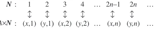
If A is a set with two objects, x and y, then A¥N is the set of ordered pairs of the form (x, n) or (y, n) for any natural number n and, by definition, it has cardinal number 2¿₀. However, this set may be put into one to one correspondence with N as in figure 5:

2n–1 :

N … …

(x,n) :

A×N _{… …}

1

(x,1)

↔ ↔

2

(y,1)

↔

3

(x,2)

↔

4

(y,2)

↔

2n

(y,n)

↔

Figure 5: A one-to-one correspondence between the natural numbers and a set with ‘twice as many’ elements

This proves that 2¿₀ = ¿₀.

A similar argument shows that n¿₀ = ¿₀ for any n Œ N. A bijection f:NÆN¥N may be defined by counting down the successive ‘backward diagonals’ as in figure 6 (where f(1) = (1,1), f(2) = (1,2), f(3) = (2,1), f(4) = (1,3), f(5) = (2,2), …). This proves that

¿₀¿₀ = ¿₀.

(1,1) (1,2) (1,3) (1,4) …

(3,1) (3,2) (3,3) (3,4) … (2,1) (2,2) (2,3) (2,4) …

(4,1) (4,2) (4,3) (4,4) …

Figure 6: ‘Counting’ the set of all ordered pairs (m,n) of natural numbers m, n

The equation ¿₀¥ x = ¿₀ therefore has solutions which include x = 1, x = 2, … and x = ¿₀. So, division by infinite cardinal numbers cannot be uniquely defined.

At this point all the examples given are of sets with the same cardinal number as the set N of natural numbers. However, for any set S, we can construct another set T whose cardinal number is strictly larger. The set T consisting of all subsets of S is a good candidate. Clearly the set S has cardinal number less than or equal to T (because the map from S to T mapping the element x to the single element subset {x} is a bijection onto a subset of T). Now consider any map f S: ÆT. We will show that it cannot map onto the whole of T. Consider the subset

K = f x( ₀). On the other hand, if x₀ œf x( ₀) then, again by definition of K, we havexŒK, once more contradicting K= f x( ₀). Thus, no map from S to T can be a bijection, so T must have a strictly larger cardinal number than S.

By repetition of this construction, we get an unending sequence of cardinal numbers, each one strictly bigger than the one before.

Ordinal numbers

Natural numbers are not only used for counting, but also for putting a (finite) set into an order, saying ‘this element is the first’, this is the second’, and so on. Just as the counting property can be extended to infinite sets using the cardinal number concept, there is an infinite extension of ordering numbers to ordinal numbers. This is done using ordered sets where a set A is said to be ordered if there is a relation denoted by a < b between some pairs of elements a, b ŒA , such that:

• Given a, b Œ A, precisely one of the following hold: a < b or b < a or a = b,

• If a < b and b < c, then a < c.

Examples of ordered sets include the set of integers Z = {…, –2, –1, 0, 1, 2, …} and the set N = {1, 2, 3, …} with their usual order.

To define the notion of ordinal number requires the ordering also to satisfy the definition: • an ordered set A is said to be well-ordered if every non-empty subset S of A has a

least element, that is there is an element l Œ S where l £ s for all s Œ S.

Of the two examples given, N in its usual ordering is well-ordered, but Z is not, because the set Z itself fails to have a least element in the given ordering.

A function f A: ÆB is said to be ‘order-preserving’ if a < b implies f(a) < f(b).

Two well-ordered sets A, B have the same ordinal number if there is an order-preserving bijection f A: ÆB.

symbol is used from the cardinal number because it happens to have very different properties, as we shall shortly show.)

1 n

:

N 2 3 … …

2 2n

:

E ↔ 4↔ 6↔ … ↔ …

Figure 7: An ordered correspondence between the natural numbers and the even numbers

We can build a mental image of a well-ordered set A, as a thought experiment, by considering successive elements in turn. Either A is empty (with ordinal number 0), or contains a least element a₁. On removing a₁, the remaining subset of elements is either empty, or contains a least element a₂. Continuing in this way, either A is finite with n elements in order a₁ < a₂ < … < an, or it contains an infinite set F of elements, a1 < a2 < … < an < … . In the latter case

there is an order-preserving bijection f:NÆF where f(n) = an, showing that the ordinal

number of F is w. Thus every well-ordered set S is either finite, or begins with a set with ordinal number w. (It can, of course have further elements that come after the elements in F in the given order.)

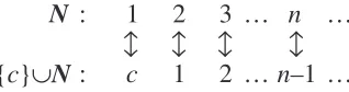
The addition of two ordinal numbers, corresponding to well-ordered sets A and B, is performed by ordering A»B by placing the elements in A before the elements in B. For instance, to obtain a set with ordinal number 1+w, we give the set {c}»N an order in which the element c comes before all the elements of N, so c < 1 < 2 < … < n for all n Œ N. This can clearly be put in a one-to-one order preserving relationship. (Figure 8.)

1 n

:

N 2 3 … …

c n–1

:

{c}∪N ↔ 1↔ 2↔ … ↔ …

Figure 8: An ordered correspondence between the two given sets

The cardinal number of {c}»N is thus the same as the cardinal number of N, giving: 1+w = w.

n ΠN. If we try to put this ordered set in one-one ordered correspondence with N, then c must correspond to some k ΠN as in figure 9.

1 < 2 < … < c

:

N∪{c} ?

… < k < k+1 < …

:

N ↔ ↔

Figure 9: There is no ordered correspondence between these ordered sets

But there is no element in N»{c} exceeding c in the order, so there is no element in N»{c} which can correspond to k+1 in N. Hence there is no possible order preserving correspondence between N»{c} and N, so w+1 is different from w. This gives the unexpected results for ordinals that

1+w = w, but

w+1 πw,

which in turn gives 1+w πw+1.

Addition of ordinals is, therefore, not commutative.

This discussion shows that cardinal infinity and ordinal infinity have different properties from each other and both differ from finite experiences of number. So strange were these ideas to the mathematical community when first announced that Kronecker prevented the initial publication of Cantor’s theory of infinite cardinals and ordinals. Such pressures subsequently caused Cantor to have a nervous breakdown. Now the theory is widely accepted but this does not make it any easier for the learner, who must negotiate a minefield of conflicting intuitions and resolve them by a reconstruction of personal knowledge. Although there are many theorems about cardinal and ordinal numbers, an intuitive grasp of their structure invariably comes after developing the formalism and reconstructing personal knowledge, not before.

‘arbitrarily large’ and ‘arbitrarily small’ numbers in the calculus. It is to this different type of infinity we now turn.

The number line

The number line is met visually in a natural embodied sense as a straight line with a chosen unit measured from 0 to 1, then repeated at equal intervals to 2, 3, … as on a ruler. (Figure 10.)

3 2

1 …

Figure 10: Numbers as points on a line

By marking negative numbers in the other direction and positive and negative fractions in between, this may be further refined to give the ‘rational’ number line. (Figure 11.)

–2 –1 0 1 2 3 …

…

–11₂ 23

Figure 11: Inserting rationals and negatives

The points on the number line are intimately connected to the line segment measured from the origin. The length of the line segment, taking direction into account, is also used to label the point as well. When students are assumed to be familiar with this idea, teachers reveal that there are points other than rational points on the number line. For, if an isosceles right-angled triangle has side-length 1, its hypotenuse is of length ÷2, and this length measured from the origin does not end up at a rational number.

At this stage, a sleight of hand occurs. As students, we are told that those points on the number line, which are not rational, are called ‘irrational’. The theoretical ‘real’ line therefore consists of rational and irrational points. In essence, this ‘explanation’ is no explanation at all! It does not say what an irrational number genuinely is, only what it is not. (It is not rational.)

can be ‘arbitrarily small’, for instance the difference between 0.999…(‘nought point nine recurring’) and 1 is extremely small, but not zero (Cornu, 1991). Most students, many teachers, and some mathematicians (certainly many physicists), do good work by imagining ‘infinitesimally small’ quantities.

The idea that there is a clearly defined ‘number line’ shared intuitively by everyone is therefore not acceptable. Despite the efforts of many mathematicians, including Cantor, to outlaw infinitesimals from mathematical analysis, they are alive and well today and continue to be used fruitfully by many experts. What we must do, therefore is to explain in what sense an ‘infinitesimal’ can be said to ‘exist’, both in a formal sense, and also as a natural embodied object that we can imagine in our mind’s eye.

Infinitesimals

… to conceive a quantity infinitely small, that is, infinitely less than any sensible or imaginable quantity, or than any the least finite magnitude is, I confess, above my capacity. (Bishop Berkeley, (reprinted 1951) p. 67.)

How can any sensible person conceive of something smaller than any sensible quantity? The answer is that we have great difficulty if we use only the perceptions of things in the world we live in. But we do not just perceive, we reflect on our perceptions to create new cognitive images within our personal cognitive structure. It turns out that many students who have experiences of quantities ‘becoming’ small in limiting processes, begin to imagine a ‘variable quantity’ that can be ‘as small as you like’ (Cornu, 1981, 1991). The language used in the calculus classroom tends to promote such thoughts, leading to individuals thinking of variables tending to zero as being ‘arbitrarily small’. Certainly, the early pioneers in the calculus thought in such terms (see Kleiner, this volume).

Ordered fields

We begin our formal journey by recalling the notion of ordered field as defined in an undergraduate mathematics course. This is given in terms of a set F with two operations +, ¥, which, for every pair of elements x, y Œ F, there are elements x+y, x¥y Œ F, where x¥y is usually written as xy. The arithmetic axioms are as follows:

• x+y = y+x, xy = yx, (x+y)+z = x+(y+z), (xy)z = x(yz) (for all x, y, z Œ F).

• There are (different) elements 0, 1 such that 0+x = 0, 1x = x for all x Œ F.

• x(y+z) = xy+xz, for all x, y, z Œ F.

• For each x Œ F there is u Œ F such that x+u = 0 and (if x π 0) there is v Œ F such that xv = 1. [The elements u and v are usually written as –x and x–1_{, respectively.]}

The ‘order axioms’ can be formulated in various ways. Here, they will be given in terms of a subset P of F (which may be considered as the ‘positive’ elements of F) satisfying the following:

• If x,y Œ P then x+y and xy are also in P.

• Every x Œ F satisfies one and only one of these properties: x Œ P, or –x Œ P, or x = 0.

The order relation x > y (also written as y < x) is then defined to hold if and only if x–y Œ P. An illustration of the axiomatic method is to use these axioms to derive the ‘usual’ order properties of the relation >. For instance, given a, b Œ F then the second property implies one and only one of the following hold:

a–b Œ P, or –(a–b) = b–a Œ P, or a–b = 0. Hence, a > b or b > a or a = b.

Given

x > y and y > z,

then

x–y, y–z Œ P,

(x–y)+(y–z) = x–z Œ P, which gives

x >z.

Hence x > y and y > z implies x > z.

This latter deduction is highly significant in terms of whether thinking is embodied or not. It establishes this order property not by the mental image of points on a line or by the Lakoff container metaphor, but by substitution of the symbols into specific order axioms prescribed for the set P.

Similar arguments allow other standard properties of order relations to be built up formally from the axioms.

If a field F also satisfies the axioms of order, then the system is said to be an ‘ordered field’. Such systems include the rational numbers Q and the real numbers R.

The real numbers also satisfy a further axiom, the axiom of ‘completeness’:

An ordered field is said to be complete if any non-empty subset S of F with an upper bound k Œ F (meaning x £ k for all x Œ S) has a least upper bound l

(that is an element l that is both an upper bound of F and smaller than any other upper bound of S).

(For further details, see for instance, Stewart & Tall, 1977).

There is an interesting reversal that occurs in formal theory. A system with more axioms usually applies to fewer examples. For instance, there are many different ordered fields, including Q and R. However, there is essentially only one complete ordered field, the familiar field of real numbers. (This follows from a structure theorem proving that, given two systems satisfying the axioms for a complete ordered field, then there is a bijection between them that is also a direct translation between arithmetic and order. In formal terms, any two complete ordered fields are isomorphic.)

There are many ordered fields, including some that contain the real numbers R as a subfield. Given that the mental image of the real numbers is essentially to ‘fill in the gaps’ on the number line (for instance using the theory of Dedekind cuts), it may come as a surprise to find that it is possible to fit in even more points than the real numbers on a visual number line.

This is addressed in the next section, by presenting a specific example of such an ordered field expressed formally. This example is given two distinct visual representations. The focus then turns to the axioms for any ordered field containing the real numbers R, leading to a structure theorem that enables us to visualize any such ordered field as a visual number line.

An example of an ordered field containing the real numbers

Consider the set R(x) of rational expressions in a variable x, of the form

a a x a x

b b x b x

n n

m m

0 1

0 1

+ + +

+ + +

K K

where the coefficients ar and bs are all real numbers, with bmπ 0. These rational expressions

have the familiar algebraic properties of addition, subtraction, multiplication and division and satisfy all the axioms for a field. Moreover, given a Œ R, by taking a₀= a, b₀= 1 and all other coefficients zero, we may consider the real numbers as a subfield R à R(x), or equivalently, seeing R(x) as a larger system containing the real numbers R.

The student may already be familiar with these expressions, simply through manipulating them in school algebra. However, our natural experience of school algebra does not put these elements in an order that turns R(x) into an ordered field. We may do this either by a formal or natural approach. The formal approach simply makes a definition of a subset P of rational functions that satisfies the properties of an ordered field, in the strict sense of Hilbert’s programme. The alternative, a natural approach, attempts first to motivate the idea with a practical example.

is to be taken as the ‘positive’ elements. As rational functions are capable of being positive in some places and negative in others, a little cunning is in order.

A rational function is either the zero function, or it is the quotient of two non-zero polynomials, each of which has only a finite number of places where it can be zero. Thus a non-zero rational function has only a finite number of points where it is zero or undefined. Take an interval 0 < x < k to the right of the origin (where k ΠR) which contains none of these places. Then in the interval 0 < x < k the function is neither zero nor infinite. It cannot be negative at one point in the interval and positive somewhere else in the interval, otherwise, being continuous, it would be zero in between. It is therefore either strictly positive or strictly negative in this interval to the right of the origin.

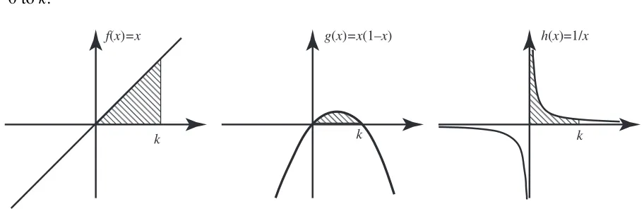
A rational function is declared to belong to P if there is a real number k such that the function has positive values for all real numbers 0 < x < k. Figure 12 shows three rational functions that are positive in an open interval to the right of the origin. The rational function f(x)=x is positive for x in an open interval from 0 to k for any positive k, g(x)=x(1–x) is

positive in the open interval from 0 to 1, and h(x)=1/x is positive in any positive interval from 0 to k.

f(x)=x g(x)=x(1–x) h(x)=1/x

k k k

Figure 12: Examples of rational functions in the set P of ‘positive’ elements (positive in an interval to the right of the origin)

This definition satisfies the axioms for an order given above and, in common with convention, we say that an element in P is ‘positive’.

in that it relates the new meaning of the term ‘positive’ to a specific visual property of a graph. This shows that formal mathematics is not a meaningless activity that only works by moving symbols around. During theorem-proving it is essential to focus on the deductive argument. However, in performing thought experiments, or interpreting formal theorems in an embodied sense, the formalism may be given any meaningful embodiment that satisfies the formal definition. This is particularly important when a given formal structure can have more than one informal embodiment.

Having defined what it means to be ‘positive’, the ‘order’ between rational functions f, g is specified by saying:

f > g if and only if f Рg ΠP.

This does not mean that the graph of f is everywhere greater than g, simply that the graph of f is higher than that of g in an interval immediately to the right of the origin.

In this new sense x > 0 and r > x for any positive real number r (because x Œ P and r – x Œ P). Thus 0 < x < r using the new order defined in the larger ordered field R(x). The element x is therefore ‘positive’ yet ‘smaller’ than any positive real number r. It is an infinitesimal.

This construction poses some possible problems. The formal learner may be satisfied with the formal symbolic approach to the definition of the ordered field R(x) and have no need for the picture. The natural learner who has a predisposition for thinking of an infinitesimal as a ‘very small quantity’ may have difficulty because the embodiment is a graph, not a number, or a point on a line.

experiment allows the novice to ‘see’ infinitesimals as ‘variable points’ that are ‘arbitrarily smaller’ than any positive real constant c. This is analogous to the notion prevalent at the beginning of the nineteenth century when Cauchy described infinitesimals as ‘variable quantities that tend to zero’.

p(x) = x2

f(x) = c

l(x) = x

P L C

x = t

Figure 13: Variable quantities seen as infinitesimals on a moving vertical line

Such an image may be helpful to some natural learners, but it can be very unhelpful to others. It fails to represent an infinitesimal as a genuine fixed point on a number line.

A formal image of an ordered field with infinitesimals as fixed points

The individual who has developed a formal concept image of an ordered field, involving only deductions from the axiomatic definition, can prove a number of formal properties that provide a context for the meaning of an infinitesimal. First one can prove the structure theorem that F contains a subfield (isomorphic to) the rationals Q. (The proof begins with 1 Œ F. Forming successive sums 1, 1+1, 1+1+1, … using an induction argument generates N, including negatives and multiplicative inverses generates the subfield Q.)

rational number x Œ Q can be infinitesimal because then r=x/2 ŒQ would satisfy r < x, contrary to the definition. A similar argument holds for x negative, so there are no non-zero infinitesimals in Q, although there may be infinitesimals in F that are not in Q.

If we try to represent the elements of F as points on a number line, we could begin by marking the elements in the subfield Q as rational points. But where do we fit the other elements of F? Our experience tells us that they might be irrationals as in R, or some other kind of element we need to think more about.

To simplify our discussion, we consider now only an ordered field F, such as R(x), which already contains all the real numbers R. An infinitesimal will then satisfy –r < x < r for all positive r Œ R. By the same argument as for Q just given, we have the following theorem:

A non-zero infinitesimal is not a real number; it is an element of a larger ordered field.

An element x Œ F is defined to be positive infinite if x > r for every r Œ R, and negative infinite if x < r for every x Œ R. A finite element x ŒF satisfies a < x < b for some a, b Œ R.

With these definitions, we can use the completeness of R to prove a structure theorem that describes the structure of any ordered field containing the real numbers:

Structure Theorem: Every ordered field F with the real numbers R as a proper subfield contains both infinitesimals and infinite elements. Every finite element is of the form c+e where c ΠR and eΠF is infinitesimal. Every infinite number is of the form 1/e where e is infinitesimal.

Proof: F has at least one element x ΠF not in R. This element x must either be finite or infinite. If x is infinite, a simple calculation shows that 1/x is infinitesimal.

If x is finite, then it satisfies a < x < b for a, b ΠR. Consider the set

S = {t ŒR | t < x}.

A visual embodiment of infinitesimals in any ordered field containing R

The structure theorem we have just proved has been established by deduction from the formal definition. It does not depend on any embodied visual properties. However, it allows us to translate the formal statement into a visual embodiment as a ‘number line’. The structure theorem implies every element of F is either infinite, which would seem ‘too far off’ in one direction or the other to see in a finite picture, or it is of the form

x = c+e, (c ŒF, e infinitesimal)

which seems ‘too close’ to c to be visually distinguishable from it.

–1/ε

(negative infinite quantity)

1/ε

(positive infinite quantity)

c–ε c+ε

c

Figure 14: An ordered field F with infinitesimals and infinite elements that seem difficult to see!

We are, apparently, in a worse dilemma than in attempting to distinguish visually between rationals and irrationals. However, unlike Bishop Berkeley, who attempted to make sense of infinitesimals purely from his perception and intellect, we have a formal image of a complete ordered field with formal structure theorem to give us support.

The problem in ‘seeing’ infinitesimals is not essentially different from the problem of ‘seeing’ distinct real numbers on the real number line. To distinguish visually between the irrational number ÷2 and the rational number 1.41421, we use a sufficiently large scale.

The same idea works for visualising the difference between c and c+e for c ΠR and e

infinitesimal. We introduce the formal function m:FÆF given by:

m

e

( )x = x-c.

0 c

c–ε

µ

c+ε

µ(c–ε) µ(c) µ(c+ε)

–1 1

Figure 15: Visualising the function m as a mapping of a number line with infinitesimals

In map-making the location of a place (eg ‘New York’) on a map is denoted by its name (New York). Replacing the names of the images by the names of the original points in the same way gives the picture in figure 16.

c c–ε

µ

c+ε

c–ε _c c+ε

Figure 16: A magnified portion of number line, showing infinitesimals

This technique allows the formal map m to be visualised in terms of a process that rescales and separates the points c and c+e.

More generally, for any a, dŒ F, the map m:FÆF given by

m a

d a d d

( )x = x- ( , ŒF, π0)

is called the d-lens pointing at a. This operation defined purely in symbolic terms, based on the operations available in a field, has a visual interpretation that maps any two points a and

representation, it is a visual interpretation of the formal construction, and, as such, has quite explicit formal properties that can be used in formal deductions.

Precisely what is seen using a d-lens can be explained using the following definition:

lΠF is of higher order detail than dΠF if l/d is infinitesimal, it is the same order if l/d is finite (but not infinitesimal) and lower order if l/d is infinite.

A d-lens pointed at a reveals details which differ from a by the same order as d; a point which differs from a by higher order difference is ‘too close’ or ‘too small’ to see, and lower order differences are ‘too far away to be seen’.

The same ideas extend to two or more dimensions using a lens on each coordinate. For instance, a d-lens pointed at (a, a2_{) reveals a nearby point (a+h, (a+h)}2_{) on the graph of y = x}2

as:

m

d d

d d d

r r r r d

( ,( ) ) ( ) ,( )

,

, / .

a h a h a h a a h a

h ah h

a h h

+ + =Ê + - +

-Ë

Á ˆ

¯ ˜

=Ê +

Ë Á ˆ ¯ ˜ =

(

)

2 where

If d is infinitesimal and h is of the same order, then r is finite and hr is infinitesimal. The standard part of the image is therefore

st( ),r st(2ar+hr) ( ,r ar2 )

(

)

Looking at the standard part of an image is the same as looking at real numbers. We define the composite of d-lens m followed by taking the standard part to be called an optical d-lens (Tall, 1980b, 1982). The finite part of the image of an optical d-lens is called the optical image. An optical d-lens maps part of a line with infinitesimal detail to a picture that reveals detail of the same order as d, as a picture in the real plane.

In the case just mentioned, the optical image is the set of points ( r, 2ar2_{) for r ΠR. This is}

precisely the real straight line, gradient 2a, through (0, 0) = m(a, a2_{). We therefore have the}

following theorem:

As the infinitesimal parts have been suppressed, the optical image is not nearly straight, but really straight.

(a+h,(a+h)2₎

(a,a2₎

(a,a2₎

optical microscope

Figure 17: Infinite magnification of infinitesimal portion of a graph as a visual image

One small step for man, one giant leap for mankind

When Neil Armstrong stepped on the moon, he moved our conceptualisation of space a great leap forward by making human imagination of the moon a reality, for himself at least. For the rest of us, of course, it is still imagination, but imagination founded on the actual experience of another.

In mathematics the step that we take in saying, ‘let there be a set N satisfying the Peano postulates,’ is one which none of us can take in actuality, for we cannot hold an infinite number of concepts in our finite mind. Yet, it is a step that many of us take easily in our imagination.

Nevertheless, there is an even greater step taken by some mathematicians, who say: Let us suppose that we have a collection of sets (possibly infinite) where none of them is empty, then simultaneously it is possible to choose a single element from each set in the collection.

the school of intuitionism, who reject it. In the latter case, all existence proofs need to involve actual constructions given by specified algorithms, as in the approach of Bishop (1967).

The twist in the tale came in the nineteen sixties when Paul Cohen (1966) proved that the axiom of choice is independent of the other axioms of set theory. Using it allows the proof of more theorems than would be possible without it, but adding it gives no new contradictions that are not present in set theory without the axiom of choice. From this viewpoint, it would seem that the intuitionist approach is just as liable to contain contradictions as a formal approach with the axiom of choice added. However, the proof of this argument uses the axiom of choice, and so it would be unlikely to be accepted from an intuitionist viewpoint.

The axiom of choice has powerful uses in analysis. For instance, it can be employed to prove the existence of a field *R called a hyperreal field, which is an extension of R and is logically appropriate to perform all the usual tasks of mathematical analysis in a field containing infinitesimals (Robinson, 1966). In this theory, each subset S of R has a ‘non-standard extension’ *S where S Õ *S Õ *R and every function f S: ÆR extends to * :*f SÆ*R where f(x) = *f(x) for all x ŒS.

In simple cases, such as an open interval

S = {x ΠR | a < x < b},

the extension satisfies the same formulae in the larger system:

*S = {x Π*R | a < x < b}.

In the same way, a polynomial function such as

f(x) = x2 _{(x ΠR)} is extended to

*f(x) = x2 _{(x Π*R).}

Other more general extensions are guaranteed by a theorem proved using the axiom of choice, essentially ‘choosing’ the extension to have the appropriate properties (e.g. Lindstrøm, 1988).

numbers N has a natural extension *N which has infinite elements. The new infinite elements in *N are called (non-standard) infinite natural numbers. If N is an infinite natural number, then so are N+1, N+2, …; N–1, N–2, …; 2N, 2N+1, … and even bigger numbers such as N2 or even NN_{, and so on. This gives a new theory of infinite natural numbers whose properties}

are quite different from Cantor’s cardinal infinities (Tall, 1980a). The non-standard natural numbers have a full and satisfactory arithmetic. If N is infinite, then N+1 is the ‘next’ natural number and is strictly bigger than N. There is a preceding natural number, N–1, and an infinitesimal reciprocal 1/N. By extending the axioms of ordered fields using the axiom of choice, we therefore get a powerful new extension to the infinite that complements the notions of infinitesimals.

This theory can be used to give powerful formal images of ideas that already appeal to the intuitive senses. For instance, any sequence (an) of real numbers is a function from N to R

and so can be extended to a function from *N to *R. The limit of the convergent sequence (an) is then the standard part of aN for any infinite element N Œ*N.

This theory gives a new way of speaking about analysis. It does not give any new theorems in everyday analysis, but it can prove them more efficiently. It does, however, give new theorems about non-standard ideas that are not part of the traditional e-d approach.

For a function f defined in an open interval containing x Œ R, then *f(x+e) can be defined for x+eŒ *R where x is real and e is infinitesimal. By computing the ratio (*f(x+e)–*f(x))/e

and taking its standard part, one can calculate the derivative of f at x. In the simple case f(x)=x2, we have

* ( ) * ( ) ( )

.

f x f x x x

x

+

-= + - = +

e e

e

e e

2 2 2

Taking the standard part suppresses the infinitesimal e and gives the derivative as 2x.

Likewise, any sequence (an) of real numbers is a function from N to R and so can be

extended to a function from *N to *R. If (an) is convergent, then the limit is defined to be the

standard part of aN for any infinite element N Œ*N. This gives an alternative approach to the

What’s in a name?

The notation of non-standard analysis is seen by some as beginning to get messy and over-fussy. For every (standard) set or function we have a non-standard extension which we notate with a preceding ‘*’. The essential fact is that, restricted to the standard case, the ‘*’ notation becomes redundant. So why introduce a new notation? Why not just extend the old one?

As ideas are extended, we invariably extend the old language to include the new. For instance, a ‘number’ may first be encountered meaning a ‘natural number’, then fractions, negatives, rationals, irrationals, even complex numbers, are all eventually called ‘numbers’.

In the same way, the name ‘real number’ may be extended to encompass the set of non-standard real numbers. Where necessary we can distinguish between the everyday real numbers by calling them standard real numbers, and the extended set non-standard real numbers. With this linguistic change, the number line can be seen in two different ways. It can be visualised as the (standard) complete ordered field R, or as a full field of non-standard real numbers with infinitesimal and infinite detail. Using optical lenses, we can visualise appropriate detail of the full (non-standard) real line as a standard real picture. In this way, we obtain a visualization of a purely formal version of this extended real line in a manner that has echoes of the intuitions of the great mathematicians in history, still found in our students today. Of course, to construct the system formally requires the individual to work through the axiomatic construction of the hyperreals using the axiom of choice (e.g. Lindstrøm, 1988; Robert, 1988). Even then, individuals may not feel that the mental construction makes sense (including those who hold an intuitionist view). Those who do achieve the cognitive reconstruction can communicate to each other about the wonders of non-standard analysis. Others must be content with an informal concept image of these powerful ideas.

The limit concept

has no role for infinitesimals, and this, wrongly, has led to a belief that there is something highly suspect about using infinitesimals. Non-standard analysis provides an alternative, which, whilst not concerning itself with the infinite cardinality of sets, has a full arithmetic of infinite integers and infinitesimal quantities.

It is therefore opportune to close this paper with a discussion of the limit concept in the light of these differing paradigms. The limit notion occurs in a number of different guises. It may involve the behaviour of a sequence of real numbers a1, a2, … , an, … as n increases, the

continuous limit of a function f(x) as x approaches a particular value a, or a more sophisticated limit such as the Riemann sum of areas of rectangles under a curve. All of these have in common a process of getting arbitrarily close to a fixed value (the limit). In every case, the same symbolism is used both for the process of convergence and also for the concept of limit. For instance

1 2 1_n

n= •

Â

evokes both the process of calculating the limit of the sum of the series and also for the numerical limiting value. Likewise

lim

x a

x a

x a

Æ

-3 3

also evokes both the process of calculating the limit as x gets close to a and also for the limiting value 3a2_.