Unsupervised colour image segmentation using dual tree complex wavelet transform

University of Warwick institutional repository: http://go.warwick.ac.uk/wrap

This paper is made available online in accordance with

publisher policies. Please scroll down to view the document

itself. Please refer to the repository record for this item and our

policy information available from the repository home page for

further information.

To see the final version of this paper please visit the publisher’s website.

Access to the published version may require a subscription.

Author(s): Turgay Celik and Tardi Tjahjadi

Article Title: Unsupervised colour image segmentation using dual-tree

complex wavelet transform

Year of publication: 2010

Link to published article:

http://dx.doi.org/10.1016/j.cviu.2010.03.002

Publisher statement: “NOTICE: this is the author’s version of a work

that was accepted for publication in Computer Vision and Image

Understanding. Changes resulting from the publishing process, such

as peer review, editing, corrections, structural formatting, and other

quality control mechanisms may not be reflected in this document.

Changes may have been made to this work since it was submitted for

publication. A definitive version was subsequently published in

Turgay Celik and Tardi Tjahjadi,

Abstract

In this paper we present an effective unsupervised colour image segmentation algorithm which uses multiscale edge information

and spatial colour content. The multiscale edge information is extracted using the dual-tree complex wavelet transform. Binary

morphological operators are applied to the edge information to detect seed regions which are large enough to exclude

boundary-only regions. The segmentation of homogeneous regions is obtained using region growing followed by region merging in the CIE

L∗_a∗_b∗ _{colour space. We also present an edge-preserving smoothing filter as a pre-process for the algorithm. We compare our}

algorithm with state-of-the-art algorithms and show its superior performance.

Keywords: unsupervised colour image segmentation, multiscale edge detection, dual-tree complex wavelet transform, discrete

wavelet transform, multiscale analysis

I. INTRODUCTION

Image segmentation is the process of subdividing an image into homogeneous regions. With colour images, the objects are

segmented with respect to their colour and spatial features. Image segmentation techniques can be categorized into two groups

[1]: soft segmentation and hard segmentations. In soft segmentation, each point in the feature space is associated with a label

whose confidence value is computed using some function related to the distance of each converged cluster. For example, Tai

et al. uses a Markov network to optimize a global objective function that combines the advantages of global colour statistics

and local contextual image statistics [1]. The method is computationally complex. The method we proposed in this paper

falls into latter category. There are four main approaches to hard image segmentation. The thresholding approach is based on

the assumption that clusters in the histogram correspond to either background or objects of interest that can be extracted by

separating these clusters [2]–[5]. Boundary-based methods assume that there is significant change in pixel properties, such as

intensity, colour and texture between different regions [6], [7]. Region-based methods assume that neighbouring pixels within

the same region have similar pixel properties [8], [9]. Hybrid methods tend to combine boundary detection and region growing

to achieve better segmentation [10]–[18].

One of the milestones in the hybrid methods is the unsupervised algorithm called JSEG [10]. JSEG uses colour quantization

and local windows to computeJ-images (corresponding to texture segmentation) at different scales. TheJ-images are combined

via multiscale region growing to obtain image segmentation. Since the computation ofJ-images requires non-linear numerical

computations, the JSEG algorithm has computational complexity which increases with the number of scales used. One drawback

of the algorithm is its sensitivity to noise. Since JSEG is based on the results of the colour quantization, another drawback is

that its performance is essentially limited by the colour quantization. The values of J-images cannot differentiate the regions

with similar distribution of textural patterns but different colour contrast results in another disadvantage of JSEG. A modified

version of JSEG proposed by Wang et al [11] uses an adaptive mean-shift clustering (AMS) for nonparametric clustering of

the image data instead of the colour quantization algorithm used in JSEG. They use Gaussian mixture modelling (GMM) of

the image data constructed with classifications obtained by AMS in the calculation ofJ-images. The segmentation results are

better in terms of better boundary representation and object segmentation. Since the method is a mixture of JSEG, AMS and

parameter estimation using GMM, it is computationally expensive.

The multiscale nature and robustness to noise of the wavelet transform makes it an attractive tool for colour image

segmentation. Multiscale edge information in non-decimated wavelet transform domain has been used with a watershed

transformation at each scale and a hierarchical region merging procedure to connect segmented regions at different scales

[12]. Although the method achieves good performance against noise, the algorithm produces oversegmented results. In [13],

multiscale image representations and watershed transforms are used. The scale-space is based on a vector-valued diffusion

scheme, and colour gradients in the YUV colour space are computed at each scale. The dynamics of the contours in

scale-space are used to validate detected contours. The segmentation results are visually pleasant but the performance of the algorithm

against noise is not determined.

Recently, decimated wavelet and watershed transforms are used to increase the robustness of an unsupervised colour image

segmentation algorithm against noise [14]. Using the horizontal and vertical subbands, a colour gradient magnitude image is

computed at the lowest resolution to detect edges. An initial segmentation map is obtained by applying a watershed transform

to the gradient magnitude image. The inverse wavelet transform is then used to project this initial segmentation to finer scales,

until the full resolution image is achieved. Finally, a region merging based on the CIE L∗_a∗_b∗ _{colour distances is applied to}

obtain the final segmentation. Since the performance of the algorithm mainly depends on the correctness of the detected edges

in the scale in which watershed algorithm is applied, further improvement can be achieved with a better edge detector. Also,

its performance depends on the watershed algorithm which requires a threshold selection process.

Multiscale edge detection could also be performed in the image domain using wavelet transform to obtain the multiscale

edge features which have good time-spatial characteristics. Mallat et al.’s approaches [19] classify singularity points as the local

maxima of gradient modulus or the zero-crossings of wavelet coefficients as edges. Sun et al. [20] used Hidden Markov Model

with wavelet transform to detect multiscale edges and fuse them to generate an edge map at the pixel resolution level for object

recognition. Zhang and Bao [21] defined a scale product as the multiplication of two adjacent scales of wavelet coefficients to

amplify edge structures while reducing noise, and using a single threshold classified the local maxima of the product as edges.

DWT-based methods generally suffers from the shift-variance and lack of directionality required in multiscale analysis to detect

multiscale edges. Wang and Jiao [22] utilised the better directionality and shift invariance of the complex wavelets, and the

scale product similar to that in [21] to detect edges. But as with most of DWT-based methods, they used wavelet coefficients

multiplication and thresholding to detect multiscale edges. There are two drawbacks with this approach. The first and the

most important is that coefficients multiplication using intra-scales may obscure low coefficients which contains information

associated with true edges. The second drawback is the dependency to thresholding. To overcome these drawbacks we propose

a Bayesian approach to detect multiscale edges using complex wavelet coefficients.

Region based merging is generally the final process for most colour image segmentation algorithms. Region merging usually

involves statistical parameters for inter and intra region correlations [23], [24] which are expensive to compute. Region adjacency

graph (RAG) [25] based merging represents each region as a graph node and an edge exists between two adjacent nodes. A

cost is assigned to each graph edge expressing the dissimilarity between two adjacent nodes. The most similar pairs of adjacent

regions until no more merging is possible. Secondly, if the number of pixels in a region is smaller than a threshold, i.e., 1/150

of the image size, the region is merged to its neighbouring region with the smallest colour distance. This procedure is repeated

until there are no regions with size smaller than the threshold. In the second pass, any two adjacent regions with size smaller

than 1/10 of the image size and the colour difference between them is greater than 0.2 are merged. This process is repeated

until no more merging is possible. The algorithm is simple and provides good results.

We proposed an unsupervised colour image segmentation algorithm to address the aforementioned drawbacks, which uses

the multiscale structure of the dual-tree complex wavelet transform (DT-CWT) [27] to detect representative edge information.

The motivation for using DT-CWT is due to its ability to detect directional edges better than DWT, increased redundancy

and the dual-tree implementation for real-time performance. The edge information is used to generate the representative seed

region for each homogeneous region in the finest resolution of the image. We employ morphological binary operators rather

than a watershed algorithm to detect seed regions in order to significantly reduce the computational complexity of the overall

algorithm. Since edge information is used to find seed regions, only a few pixels are not assigned to any seed region. Thus,

the pixel assignment performed by the region growing is computational inexpensive. A region growing and region merging

are then applied to obtain the overall segmentation. The region merging is performed in the uniform CIE L∗_a∗_b∗_{colour space}

[28] to address oversegmentation. We also introduced a new edge-preserving smoothing filter which is used as a pre-process

for the algorithm.

The paper is organized as follows. Section II presents the proposed algorithm. Section III presents the experimental results

and discussions. Finally, Section IV concludes the paper.

II. PROPOSEDALGORITHM

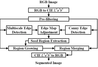
Figure 1 shows the overview of the proposed algorithm. The first stage of the algorithm transforms the image from the RGB

to the CIE L∗_a∗_b∗ _{colour space. The second stage smoothes the image using a non-linear pre-filtering operation (see Section}

II-A). The aims of the pre-filtering are two folds: to remove small variations in the input image while retaining a contrast

between different regions; and to reduce the noise level.

A multiscale edge map is found using DT-CWT (see Section II-B and II-C) and combined with the result of a Canny edge

detection to detect finer boundary edges. The resulting edge map is used to find seed regions that correspond to regions to be

segmented (see Section II-D). Since the seed regions do not fully encompass their corresponding region, a region growing (see

Section II-E) is applied. Since the region growing may produce oversegmentation when a sub-region is incorrectly segmented

as more than two spatially neighbouring regions, a region merging (see Section II-E) is also applied. When every region has

been segmented and represented with an average colour (pseudo-colour) vector in the CIE L∗_a∗_b∗ _{colour space, an inverse}

image transformation is performed to convert the segmented image to its RGB representation.

A. Pre-filtering image

A commonly used pre-filter is a Gaussian or weighted mean filter. However, the noise reduction is achieved at the expense

Fig. 1. Proposed colour image segmentation algorithm.

adaptive mean filter) where the amount of blurring of each pixel is determined from the local information in a specifiedn×n

neighbourhood. Tomasi and Manduchi’s bilateral filter [29] is the state of the art for edge-preserving smoothing. The filter

combines grey levels or colours of pixels based on both their geometric closeness and their photometric similarity. The main

drawback of this method is the need to tune parameters for domain filtering (σd) and range filtering (σr). It also necessary to

specify the bilateral filter half-width (w). Different parameters generate different filtering results, and bilateral filtering provides

excellent results with a good choice of parameters but requires high computation for each pixel.

For an unsupervised filtering which does not require any parameter selection, we propose an edge preserving smoothing

filter (EPSF) which employs adaptive filter coefficients for each pixel value. The coefficients are

ci= exp (−di) (1)

where di, i= 1. . .24 are the colour distances between the centre pixel and its neighbouring pixels, normalized to the range

of[0 1], i.e.,

di= r

(L∗

c−L∗i)2+ (a∗c−a∗i)2+ (b∗c−b∗i)2

3 (2)

where (L∗

c, a∗c, b∗c) and(L∗i, a∗i, b∗i) are respectively the CIE L∗a∗b∗ colour values of the centre pixel and its neighbouring

pixels. For a neighbouring pixel, the corresponding coefficient is high if its colour value is close to the value of the centre

pixel, and vice versa.

A dynamic5×5 mask centred at spatial location(x, y)is defined as

T(x, y) = _P241

i=1ci 2

4

c1 c2 c3 c4 c5

c6 c7 c8 c9 c10

c11 c12 0 c13 c14

c15 c16 c17 c18 c19

c20 c21 c22 c23 c24 3

5. (3)

The filtering of the image is achieved by convolving the maskT(x, y)with each of the CIEL∗_a∗_b∗_{components separately. As}

(a)

(b) (c) (d)

(e) (f) (g)

Fig. 2. EPSF filtering of House image: (a) Original image; (b) After Eq. (4) is applied once; (c) After EPSF is applied once; (d) After bilateral filtering [29] is applied once; (e) After Eq. (4) is applied 5 times; (f) After EPSF is applied 5 times; and (g) after bilateral filtering [29] is applied 5 times.

value from coefficients with large colour distance, thus reducing any blurring. The centre pixel of the mask is set to0 in order

to remove impulsive noise. Note that when EPSF is applied to object edge pixels, the colour distances di are large for the

neighbouring pixels that do not belong to the object and hence the colours of these neighbouring pixels have a small effect

on the final colour of the centre pixel. Thus, the proposed filter is considered as an edge preserving filter. Note also that the

size of EPSF may be extended to any n×nsize by following a similar methodology. However, as the filter size is increased

the blurring is also increased.

Figure 2 shows the effects on an image when EPSF is applied once, iteratively, and with constant EPSF coefficients, e.g.,

T(x, y) = 1 44

2

6 4

1 1 2 1 1 1 2 4 2 1 2 4 0 4 2 1 2 4 2 1 1 1 2 1 1

3

7

5. (4)

It also shows the application of the bilateral filter in [29] with parameters w = 2, σd = 3, σr = 0.1. Note that w = 2 is

selected in order to use the same local spatial support, and other parameters are tuned to give a good performance. As is

seen mainly from the pixel profiles around object boundaries, noise is reduced almost without blurring by using both bilateral

filtering and EPSF. However as the number of iterations increases EPSF retains higher contrast than bilateral filtering at region

boundaries. More iterations will remove more noise but at the expense of loosing details around object boundaries. We found

that 5 iterations are sufficient to reduce noise without blurring.

Figure 2 shows that even when an image is not noisy, EPSF retains the contrast between regions but removes some small

details within a region, e.g., the shape of the individual bricks within a wall region are no longer recognizable. However, it is

expected that if the image is noisy, then EPSF should remove noise while retaining clear region boundaries. Figure 3 shows

the effects of applying EPSF with constant coefficients, EPSF with dynamic coefficients and bilateral filtering on a noisy

House image using 5 iterations. Figure 3 shows that EPSF and bilateral filtering are good at removing noise and retaining

(a) (b) (c) (d)

Fig. 3. EPSF filtering of a noisy image: (a) Original image with added Gaussian noise (SNR = 26 dB); (b) After (Eq. (4)) is applied 5 times; (f) After EPSF is applied 5 times; and (g) after bilateral filtering [29] is applied 5 times.

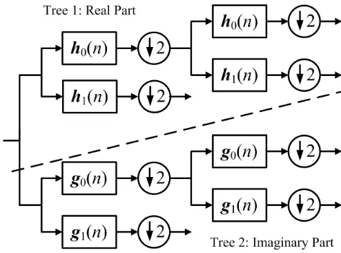
Fig. 4. Two-level 1-D dual-tree complex wavelet transform (DT-CWT).

absence of noise, EPSF retains a higher contrast between regions.

B. Dual-tree complex wavelet transform

The ordinary DWT is shift variant because of the decimation operation exploited in the transform. As a result, a small

shift in the input signal can cause a very different set of wavelet coefficients produced at the output. For that, Kingsbury

[27] introduced a new kind of wavelet transform, called the dual-tree complex wavelet transform (DT-CWT), which exhibits

approximate shift invariant property and improves directional resolution when compared with that of the DWT. At each scale,

the DT-CWT produces six directional subbands, oriented at _±15◦_,±45◦_{, and ±75}◦_{, while the DWT produces only three}

directional subbands, oriented at0◦_,45◦_{, and90}◦_.

The DT-CWT also yields perfect reconstruction by using two parallel decimated filter-bank trees with real-valued coefficients

generated at each tree. The one-dimensional (1-D) DT-CWT decomposes the input signalf(x)by expressing it in terms of a

complex shifted and dilated mother waveletψ(x)and scaling functionφ(x); that is,

f(x) =X l∈Z

sj0,lφj0,l(x) +

X

j≥j0

X

l∈Z

cj,lψj,l(x), (5)

whereZis the set of natural numbers,jandlrefer to the index of shifts and dilations respectively,sj0,lis the scaling coefficient

and cj,l is the complex wavelet coefficient with φj0,l(x) = φ r j0,l(x) +

√ −1φi

j0,l(x) and ψj,l(x) = ψ r j,l(x) +

√ −1ψi

j,l(x),

(a) (b) (c) (d) (e) (f)

(g) (h) (i) (j) (k) (l)

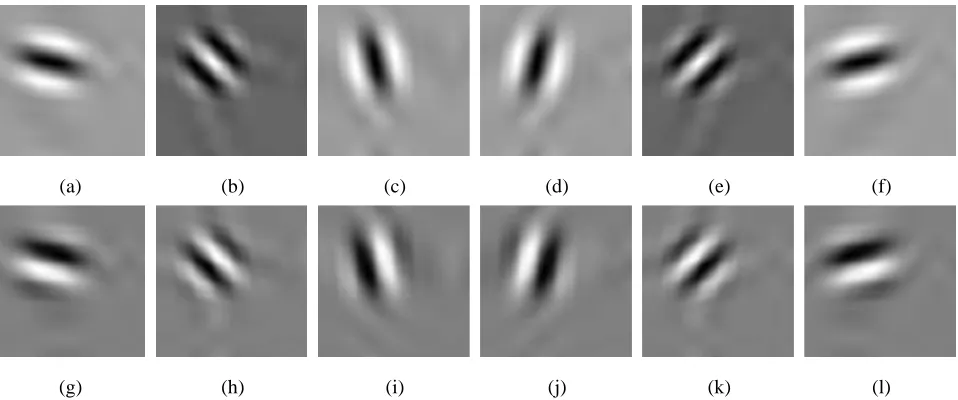
Fig. 5. The real (R) and imaginary (I) parts of the impulse responses of the 2-D DT-CWT filters under 6 directional subbands: (a)R−15◦; (b)R₋₄₅◦; (c)

R−75◦; (d)R₊₇₅◦; (e)R₊₄₅◦; (f)R₊₁₅◦; (g)I₋₁₅◦; (h)I₋₄₅◦; (i)I₋₇₅◦; (j)I₊₇₅◦; (k)I₊₄₅◦; (l)I₊₁₅◦.

Fig. 6. Frequency-domain partition resulted from a two-level 2-D DT-CWT decomposition, wherewR andwI are the real axis and the imaginary axis of

the complex frequency domain, respectively.

{φr j0,l, φ

i j0,l, ψ

r j0,l, ψ

i

j0,l} forms a tight wavelet frame with double redundancy. The real and imaginary parts of the 1-D

DT-CWT are computed using separate filter banks with filters h0 andh1 for the real part, and g0 andg1 for the imaginary part,

as illustrated in Figure 4 [27]. The outputs from the two trees in Figure 4 are interpreted as the real and the imaginary parts

of the complex coefficients.

Similar to the 1-D DT-CWT, the two-dimensional (2-D) DT-CWT decomposes a 2-D image f(x, y) through a series of

dilations and translations of a complex scaling function and six complex wavelet functions ψθ j,l, i.e.,

f(x, y) = X l∈Z2

sj0,lφj0,l(x, y) +

X

θ∈Θ

X

j≥j0

X

l∈Z2

cθ j,lψ

θ

j,l(x, y). (6)

where θ ∈ {±15◦_, ±45◦_,

±75◦

f(x, y)by exploiting the DT-CWT produces one complex-valued low-pass subband and six complex-valued high-pass subbands

at each level of decomposition, where each high-pass subband corresponds to one unique direction θ. The impulse responses

of the six complex wavelets of the 2-D complex wavelet transform are illustrated in Figure 5. The frequency-domain partition

resulted from a two-level 2-D DT-CWT decomposition is graphically shown in Figure 6.

C. Generating multiscale edge map using DT-CWT

Edges between regions are expected to be present even when the image is processed via different scales and different

orientations. Interscale features of DT-CWT with 6 different orientations may be used to extract edges with different orientations

in different scales. The coefficients in the subbands may be modelled using Gaussian distributions or a mixture of Gaussians. The

latter requires the weights and parameters of each distribution and thus requires high computational time for the corresponding

model. However, if the norm of each complex coefficient in a subband is used, which is a form of a nonlinear transformation

of the coefficients, the overall distribution for the coefficients within a subband may be modelled with the Rayleigh distribution

[30]. Scharcanski et al. only used LH and HL subbands to estimate gradient magnitude and direction in each scale [30]. The

estimated gradient information is enhanced using scale and space consistency. Unlike their method, we model the magnitude

of each complex subband coefficient in DT-CWT as Rayleigh distribution. Since at each scale, DT-CWT has 6 subbands, we

have 6 different sources of information whereas the DWT based method in [30] provides only a single source of information.

Unlike the method in [30] we define the test statisticsGRθCθ =

p

Rθ2+Cθ2, θ=±15◦,±45◦,±75◦.RθandCθare the

real and imaginary coefficients with the same directionality in each subband respectively. The distribution of the test statistics

follows the Rayleigh distribution. The distribution ofGRθCθ consists of edges and non-edges. Non-edge information represents

homogeneous texture information and the edge is the passage between regions. Thus,GRθCθ consists of two classes: ce and

cne, where the first represents the edges and the second represents the non-edges which may be considered as homogeneous

regions, i.e., non-edge regions. The distribution of ce is approximated by

pRθCθ(r/ce) =

r σ2

e

e−r2/(2σe2) ₍₇₎

wherer∈GRθCθ andσ

2

e is the parameter for its Rayleigh distribution. Similarly the distribution ofcne is

pRθCθ(r/cne) =

r σ2 ne

e−r2/(2σ2ne) ₍₈₎

where σ2

ne is the parameter for its Rayleigh distribution. The overall distribution of GRθCθ is approximated by a linear

combination of distributions of the two classes, i.e.,

pRθCθ(r) =πe pRθCθ(r/ce) +πne pRθCθ(r/cne) (9)

whereπeandπne are the weights of the corresponding classes andπe+πne= 1.

In order to estimate the distributions forceandcnethe corresponding parametersπe,σ2eandσ2neare estimated by maximizing

the likelihood function

ln (L) = X

all(x,y)

ln (pRθCθ(GRθCθ)). (10)

Using the optimization in Eq. (10) the following iterative equations are derived for estimating πe,σe2 andσne2 :

τni(t) =

πit rσn2 i e

−r2 n/(2σ2i)

P jπjt rσn2

j

e−r2n/(2σj2)

(11)

σi(t+ 1) = P

nτni(t)rn2

2P nτni(t)

0 0.05 0.1 0.15 0.2 0

0.005 0.01

p

r

0 0.005 0.01

r 0 0.05 0.1 0.15 0.2

0 0.005 0.01

r pR−15C−15(r) pR−45C−45(r) pR−75C−75(r)

0 0.05 0.1 0.15 0.2

0 0.005 0.01 0.015 0.02 0.025 0.03 0.035 0.04 p R +75 ° C+75 ° (r)

r 0 0.02 0.04 0.06 0.08 0.1 0.12

0 0.005 0.01 0.015 0.02 0.025 0.03 0.035 0.04 pR +45 ° C +45 ° (r) r

0 0.05 0.1 0.15 0.2

0 0.005 0.01 0.015 0.02 0.025 0.03 0.035 0.04 0.045 pR +15 ° C +15 ° (r) r

pR+75C+75(r) pR+45C+45(r) pR+15C+15(r)

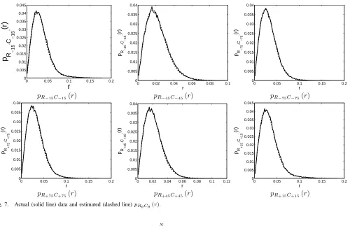
Fig. 7. Actual (solid line) data and estimated (dashed line)pRθCθ(r).

πit+1=

1 N

N X

n=1

τni(t), i=ce, cne (13)

where t and t+ 1 are respectively the current and next iteration, and N is the total number of coefficients in GRθCθ. The

correct estimation of these parameters is crucial for the success of the edge detection. Figure 7 shows the actual distribution

ofpRθCθ(r)and its estimation usingπe,σ

2

e andσne2 for the 6 directional subbands for the House image in the second scale of

DT-CWT domain. Note there is a close agreement between the actual and estimated distributions. Once the parameters have

been accurately estimated, the Bayes theorem is used to estimate the conditional distributions forceandcne as follows:

pRθCθ(ce/r) =

πepRθCθ(r/ce)

P

jπjpRθCθ(r/cj)

(14)

pRθCθ(cne/r) =

πnepRθCθ(r/cne)

P

jπj pRθCθ(r/cj)

. (15)

Using pRθCθ(ce/r) the edge map for the corresponding scale is computed by using a combination of all edge maps in all

subbands, i.e., the overall edge map in a given scale is defined as ps(ce/r)and is equivalent to the maximum of all edge

maps in all subbands, i.e.,

ps(ce/r) = max n

pRθCθ(ce/r)θ∈{±15,±45,±75} o

(16)

where s corresponds to the scale. Note that max_{} may generate false alarms for a given scale s, but the false alarms are

reduced by the multiscale nature of DT-CWT.

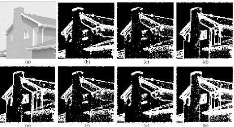
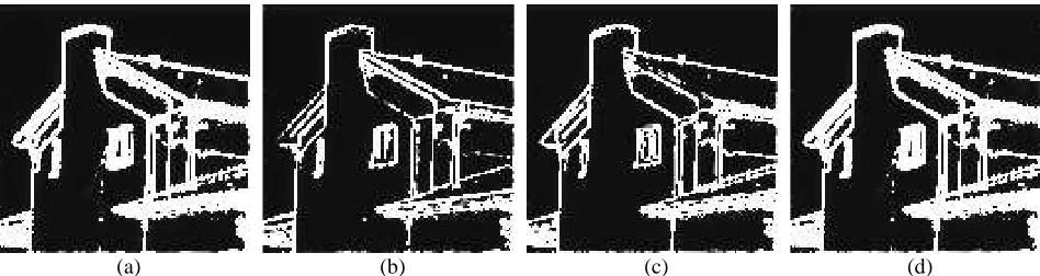
Figure 8 demonstrates the extraction of the overall edge map for an image using Eq. (16). It is clear that different subbands

detect different types of edges, i.e., different directionalities in DT-CWT produce different edges. The combination of edge

maps,ps(ce/r), produces an edge map for a corresponding scales, which provides the contours for region boundaries. Figure 8

also shows that the edges detected in subbands provide reasonable edge maps and the model proposed in Eq. (16) generates

(a) (b) (c) (d)

(e) (f) (g) (h)

Fig. 8. Edge map for scales= 1using the maximum of subband edge maps: (a)L∗_{component of image in Figure 2(f); (b)-(g) Edge maps in 6 directional}

subbands; and (h) Overall edge map using Eq. (16).

through the consecutive scales, i.e., interscale continuum of the pixel is guaranteed if the pixel is an edge pixel, we propose

ps(ce/r) =f(ps(ce/r), ps+1(ce/r)) (17)

wheref(,)is any function which may be used for enhancing the edge map using scales ofsands+ 1. In [30] it is proposed

thatf(a, b) = 2/(1_a +1_b), where it is assumed that if a pixel has a high edge dependency than the edge dependency should

also be high at the corresponding spatial location in the next scales+ 1. For example, ifa=1,b=1 (i.e., the corresponding pixel

is an edge pixel at both scales sands+ 1) then the likelihood of the corresponding updated edge pixel at scale sbecomes

f(a, b) = 1. If a=1, b=0.5 (i.e., the corresponding pixel is an edge pixel at scale s and the likelihood that it is defined as

an edge pixel at s+ 1is half) then the correspondingf(a, b) = 0.67 is smoother for a correspondingps(ce/r). This means

that if a pixel is defined as an edge pixel at a finer scale (i.e., image resolution) and the likelihood that it is an edge pixel

reduces to half of the maximum value for the next resolution, then the likelihood at a finer resolution retains this interscale

dependency. Each edge map is then updated using the iterative formula

pus(ce/r) =f(pus+1(ce/r), ps(ce/r)) (18)

s =S−1, . . . ,1, wherepu

s(ce/r)is the updated edge map and S is the number of scales used. Figure 9 demonstrates the

update of an edge map Figure 9(b) (generated using only Eq. (16)), which consists of high detailed edges and numerous

false detections. The false detections are reduced in Figure 9(c) by using Eq. (18), clearly showing that Eq. (18) brings the

multiscale edge continuum to the current scale with nonlinear functionality. Although some details are lost, the edge information

is enhanced and false detections are reduced. Since a colour image is used, the overall edge map is

ps,all(ce/r) = max(pus,L∗(ce/r), pus,a∗(ce/r), pus,b∗(ce/r) ) (19)

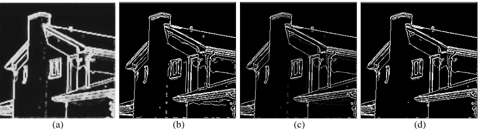
i.e., the maximum of the edge map of each of the CIE L∗_a∗_b∗ _{components. Figure 10 shows the edge detection using}

(a) (b) (c)

Fig. 9. Final edge map ats= 1by using the iterative edge map update: (a) Original image; (b) Original edge map; and (c) Updated edge map.

(a) (b) (c) (d)

Fig. 10. The union of edge maps from all colour channels: (a)L∗_{channel; (b)a}∗_{channel; (c)b}∗_{channel; and (d) Overall edge map using Eq. (19).}

edge map is constructed with s= 1, i.e., at the finest resolution of DT-CWT. We use bilinear interpolation to resize the edge

map to the original image size. Due to the blocking effect in interscale edge detection and bilinear interpolation, the enlarged

edge map produces thick edges. Thus, the Canny edge detector is applied to all colour channels to thin the edges.

The overall edge map detected by Canny edge detector is given by

eL∗_a∗_b∗ = Φ (L∗)∪Φ (a∗)∪Φ (b∗) (20) whereΦ ( )refers to the Canny edge detector. Since the Canny edge detector produces binary results,eL∗a∗b∗ is a binary map

where 0 represents no edge and 1 represents an edge. The overall edge map in the image domain is simply the multiplication

ofeL∗_a∗_b∗ with the upscaled version ofp_1,all(c_e/r), i.e.,

pL∗_a∗_b∗(ce/r) =eL∗_a∗_b∗×Θ (p_1,all(ce/r)) (21)

whereΘ ( )refers to the upscaling function using bilinear interpolation.

The edge map obtained using Eq. (21) represents a value in the range of [0 1], where a value close to 1 means stronger

edges, and vice versa. In order to classify a pixel into one of the two classes (ce, cne), i.e., to generate the overall binary

edge map BEM, Otsu’s automatic thresholding method [4] is used since the proposed algorithm is unsupervised. The Otsu’s

method is quite successful in thresholding a given data into two classes. The threshold is automatically determined and is set

to the value which maximizes the discrimination criterion σ2

B/σw2

, where σ2

B is the between-class variance and σ2w is the within-class variance. In Figure 11(a) the upper left window is detected as part of the upper left roof frame, but after applying

(a) (b) (c) (d)

Fig. 11. Using Eq. (21) for the image in Figure 2(f): (a)Θ`

p1,all(ce/r)´; (b)eL∗a∗b∗; (c)pL∗a∗b∗(ce/r); and (d) BEM.

Fig. 12. Sample results for Canny edge detector and BEM: (row 1) Original images; (row 2) using only Canny edge detector; and (row 3) BEM.

BEM (Figure 11(d)) the Canny edge detector is applied with its upper and lower thresholds set to 0. However, we note that

since different types of images have different types of edges which can only be detected by using different sets of thresholds,

it is not possible to use a single set of thresholds which is effective for all images.

Figure 12 shows some edge detection results using the Canny edge detector eL∗a∗b∗ with manually selected optimum

thresholds for different types of images. Note that, the two thresholds for the Canny edge detector also used in generating

BEM are always set to 0. Figure 12 shows that unlike BEM (generated by the proposed multiscale edge detector), using only

the Canny edge detector produces false detection for the highly textured areas.

D. Detecting seed points to represent colour image regions

The homogeneous colour image regions are represented by seed points and each cluster of connected seed points corresponds

to a region of colour or texture dissimilar to other neighbouring regions. The regions are segmented into disjoint areas using

the multiscale edge information given by Eq. (21) and their BEM. Thus, the region edge information is used to identify seed

points. Note there are no edges within a homogeneous region. Seed points are detected using the following rules: if a pixel is

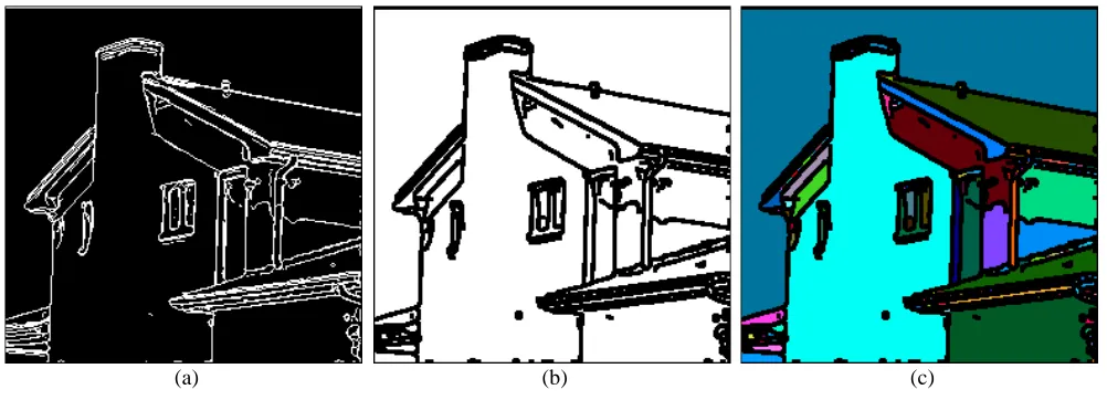
(a) (b) (c)

Fig. 13. Seed extraction: (a) BEM in Figure 11(d); (b) SM; and (c) ColouredSi’s.

pixel, i.e.,

SM(x, y) =

8

> <

> :

1 if (TEM(x, y)≡₀₎

0 otherwise

(22)

where TEM(x, y) =P1

u=−1

P1

v=−1BEM(x+u, y+v), and SM is a seed map with seed points labelled as 1 (white) and

non-seed points labelled as 0 (black), and(x, y)is a spatial pixel location.

It is clear from Figure 13(b) that each region in House image is represented by a group of seed points. In order to group

all the seed points detected within each region to obtain a single representative seed region Si, an algorithm based on the

connected component labelling algorithm [31] is used to generate a label matrix LM. The algorithm is a two-pass process. At

the start of the process all labels in LM and the current label iare initialised to 0. In the first pass, SM is examined from its

upper-left to its lower-right corner. When the current pixel at (x, y)is found to be ON (i.e., SM(x, y) = 1), the neighbouring

pixels to its left ((x−1, y)), top ((x, y−1)), top-left ((x−1, y−1)) and top-right ((x+ 1, y−1)) are examined. The following

three situations can occur: none of these neighbours is ON, and a new label (equals to the value of current labeliincremented

by 1) is assigned to the current pixel in LM; one of the neighbours is ON, and the current label is set to the label of that

neighbour and assigned to the current pixel in LM; and more than one neighbours are ON, the current pixel in LM is set to

one of the labels, and all labels of these neighbours are put in an equivalence class to indicate that these labels correspond

to the same region on the basis of being connected. After the first pass is completed, all labels in each equivalence class are

merged to a single label. After this process, each regionSi is represented by a labeli. Figure 13(c) shows the 144 seed regions

(Si) obtained by applying the labelling algorithm on SM.

E. Region growing using seed regions and region merging

Each connected seed regionSi is grown and all pixels that are labelled as non-seed (e.g., the black pixels in Figure 13(b))

are assigned to the appropriate seed region. The region growing algorithm is as follows:

1) Create a link-list of neighbouring pixels for each seed region, and sort each link-list in ascending order with respect to

the minimum colour distance of each pixel to its neighbouringSi’s.

2) Remove the first element of each link-list which has the smallest distance to its nearest neighbouring seed region and

(a) (b)

Fig. 14. Effect of region growing on seed regions: (a) Coloured seed regions; and (b) Result of region growing.

add the removed pixel’s unlabelled neighbouring pixels to the link-list with respect to their distance to the nearest seed

region.

3) Go to step 2 while there are elements in link-list to process.

Let D(p1, p2, p3) =

p p2

1+p22+p23 and use ∆ =

D((L∗

r−L∗Si),(a∗r−aSi∗ ),(b∗r−b∗Si)) D(L∗

r,a∗r,b∗r) as the colour distance between pixel r with (L∗

r, a∗r, b∗r) and regionSi with region mean colour (L∗Si, a ∗ Si, b

∗

Si). Other criteria may be used in region growing, e.g,

the nearest pixels with the original colour value. But this results in an increase in memory requirement and computational

complexity. Since the region growing is a process which needs high computation, its load should be kept as low as possible.

Thus we applied the mean region colour as the only similarity criterion. After region growing is applied, each seed regionSi

is grown to beRi. The region growing process combats the enlargement of edges caused by the seed selection process. This is

illustrated in Figure 14. Note that the black pixels in Figure 14(a) are merged with the coloured regions due to their similarity

in colour. Figure 15 demonstrates the results of the region growing, where each regionRi is coloured with the average colour

of the corresponding region. Note that there is an oversegmentation which is removed by region merging.

The region merging handles any oversegmentation by merging neighbouring regions that satisfy the merging conditions. A

region should be merged to its neighbouring region with similar colour, i.e., the colour distance between them is smaller than

a predefined threshold, and if its size is smaller than a predefined threshold. The size threshold becomes important if two

neighbouring regions have similar colour but their sizes are not small, e.g., a sky region should not be merged with a sea

region.

The merging algorithm in [26] is modified and used as follows. The YCbCr colour space used in [26] is replaced with

CIE L∗_a∗_b∗ _{since the latter provides better colour difference metrics. Two adjacent regions (R}

i,Rj) with the smallest colour

distance among all regions are examined first. In each iteration, if the distance is smaller than a threshold then the regions

are merged. The mean colour of the merged region, and distances between the merged region and its neighbouring regions

are re-calculated. This process is repeated until no two adjacent regions have colour distance smaller than the threshold. The

colour distance [26] between two adjacent regions Ri andRj is re-defined as

d(Ri, Rj) =

D“(L∗ Ri−L

∗ Rj),(a

∗ Ri−a

∗ Rj),(b

∗ Ri−b

∗ Rj)

”

min“D(L∗ Ri, a

∗ Ri, b

∗ Ri), D(L

∗ Rj, a

∗ Rj, b

∗ Rj)

” (23)

where(L∗ Ri, a

∗ Ri, b

∗

Ri), and(L ∗ Rj, a

∗ Rj, b

∗

Rj)are the mean colour of regionRiandRj, respectively. The threshold value for the

Fig. 15. Original and pseudo-colour representation of segmented images after region growing.

due to their small size. In order to remove this artifact, while merging with respect to region sizes, a second threshold is used

and which is set to 0.15. This procedure is repeated until no regions have size smaller than the threshold. The size threshold

used in this merging step is 1/150 of the total number of pixels in an image.

Figure 16 demonstrates the region merging. Figure 16(d) shows the result of merging adjacent regions with colour distance

smaller than 0.1, where similar regions but segmented differently in Figure 16(c) are merged together. Figure 16(e) shows

further merging of regions with size smaller than 1/150 of original image size to adjacent region with the smallest colour

distance. The result consists of similar regions that should be merged together, i.e., these are results of oversegmentation. In

order to achieve a better segmentation and to overcome oversegmentation, the same merging strategy is applied with different

thresholds. In the second stage: the colour distance is set as 0.15 to prevent the algorithm from merging different regions

whose sizes are suitable for merging; and the size threshold is set as 1/50 of the total number of pixels in an image. Similar

to the first stage, the size threshold is used in conjunction with the other condition of colour distance threshold of 0.225 to

prevent merging of small sized regions that should not be merged. This is unlike the method in [26] which does not check

for colour difference when merging regions with respect to size and thus may merge regions which are small in size but have

very high contrast. Our method prevents adding very high contrast regions to the mean representation of big sized regions.

The oversegmentation in Figure 16(e) is reduced in Figure 16(f) by the second stage.

The thresholds used in region merging affect the overall segmentation. If the colour distance threshold is too high then some

different regions may be merged together; conversely there will be too many regions. Similarly for the size threshold: too high

(a) (b) (c)

(d) (e) (f)

Fig. 16. Demonstration of region merging: (a) Original image; (b) Seed pixels are depicted in red; (c) Result of region growing; (d) Result of merging adjacent regions with colour distance smaller than 0.1; (e) The result of merging small regions with size smaller than 1/150 of the image; and (f) Final segmented image using further steps in region merging with different colour distance threshold of 0.15 and size threshold of 1/50 of the overall image size.

ad-hoc but better values are obtained if the content of the image is considered. For example, if the image contrast between

regions is not high, than it would be better to set the colour distance thresholds as small as possible; and if there are small

sized objects in the image, then the size threshold should be as high as possible to prevent losing objects.

III. EXPERIMENTAL RESULTS AND DISCUSSIONS

The performance of the proposed algorithm is evaluated using 300 natural images from the Berkeley dataset [32]. The

performance is compared with that of JSEG [10] and Mean-shift [15]. The number of scales for both the proposed algorithm

and JSEG is set as 3 and no other parameters are changed in the tests. The default optimum threshold values used for every

image in [10], [15] are used for both JSEG and Mean-shift. For JSEG the colour quantization threshold is set to “automatic

selection”, the region merge threshold is set to 0.4, and the number of scales is set to “automatic selection”. Mean-shift is a

unified approach for colour image denoising and segmentation which uses a kernel in the joint spatial-range domain to filter

image pixels in the CIEL∗_u∗_v∗_{colour space. The filtered pixels are clustered to segment the objects. The algorithm requires}

a selection of spatial(hs)and colour(hr)bandwidths, and optionally a minimum area parameterM for region merging. The

parameters(hs, hr, M) = (7,6.5,20)are used for Mean-shift.

To compare the performance of the three algorithms quantitatively different measures are used. One measure is the peak

signal to noise ratio (PSNR) between the original image and the pseudo-colour representation of segmented image, i.e.,

PSNR=1

3

3 X

i=1

10 log_{10 1} 1

K PK

x=1(Ii(x)−Iˆi(x))2 !!

(24)

where Ii and Iˆi are respectively the ith, i ∈ {R, G, B}, colour channel values of the original image and pseudo-colour

representation of the segmented image, x is spatial location and K is number of pixels in the image. Both Ii and Iˆi are

normalized to1. A high value of PSNR is highly likely to indicate that the original and pseudo-colour representation are quite

for the algorithm. Precision is the fraction of detections that are true positives rather than false positives, while Recall is the

fraction of true positives that are detected rather than missed. Precision is a measure of how much noise is in the output of

the detector and Recall is a measure of how much of the ground truth is detected. Even though these two quantities are good

indicators for boundary representation, a single measure is required to show how good the segmented boundary is. Thus,

F = P×R

(α×_{R+ (1}−_α)×_P) (25)

whereαis a threshold and set to 0.5 as is used in [33]. The higher the value of F the better is the boundary representation.

Figure 17 clearly shows that the proposed algorithm (using default threshold values) is better in segmenting region boundaries

when compared to the other algorithms (also using their default threshold values). The second row of Figure 17 shows a scene

which consists of similar coloured objects where the contrast between object boundaries is not high, e.g., the contrast between

some branches of tree and mountain. Even with this image condition, the proposed algorithm correctly detects most of the

different objects in the scene, i.e., the branches, sea and mountain. Note that the oversegmentations are noticeble in the results

by Mean-shift and there are missing boundaries in the results by JSEG. For example, in the first row JSEG segments the House

image into 31 regions and fails to detect the upper left window, the left guttering which is extended toward a wall, and a small

green plant near the left guttering. Furthermore the region boundaries are not sufficiently smooth. These missing regions are

well detected by Mean-shift. However Mean-shift segments the image into 124 regions. This oversegmentation gives visibly

pleasant result but poor regional representation. These drawbacks are overcome by the proposed algorithm which segments the

House image into 32 regions, where regional information is retained with good boundary representation.

Table I shows the values of PSNR, number of segmented regions Nr, P, R and F for the images in Figure 17. In terms

of PNSR, the performance of the proposed algorithm is second to Mean-shift. However, Mean-shift produces the most

oversegmentation. Also, the number of segmented regions for JSEG and the proposed algorithm is about the same. This

effect is reflected through the values of F for which our algorithm gives the highest (i.e., best) values. For instance Mean-shift

segments Lena image (row 4 of Figure 17) into 354 regions and achieves the best PSNR value, but most of these regions

are over-segmentation and should be merged. It is visually clear that Lena image does not has 352 regions, it thus means

Mean-shift produces a large number of false positives. On the other hand, it also produces a large number of true positives. For

this reason, the value of P, R and F are respectively 0.47, 0.98, and 0.64. On the other hand the values of F for the JSEG and

the proposed algorithm are 0.69 and 0.75, respectively. This is mainly due to the low false positive rates of the two algorithms

with respect to Mean-shift. Thus, the proposed algorithm achieves the best overall performance.

The performance of the proposed algorithm in the presence of different levels of noise is also evaluated and compared

with JSEG and Mean-shift. The 512x512 House image (i.e., top-left image in Figure 17) contaminated with different levels

of zero-mean Gaussian noise is used as the test image. The PSNR between the original House image and the segmentation of

each noisy House image (for various noise levels) is calculated (for each of the three methods). The Nr, P, R, and F in each

of the segmented images are also calculated. Table II shows that the values of PNSR, Nr, P, and F for Mean-shift deteriorate

the most as the noise level is increased, thus indicating that the method is the least robust against noise. The change in values

2 18.32 39 0.73 0.84 0.78 22.73 337 0.51 0.98 0.67 19.94 66 0.70 0.88 0.78 3 23.38 29 1.00 0.96 0.98 26.45 113 0.91 1.00 0.95 24.83 37 0.99 0.99 0.99 4 21.59 64 0.58 0.86 0.69 24.93 354 0.47 0.98 0.64 22.01 53 0.65 0.89 0.75 5 19.79 74 0.52 0.9 0.66 24.24 456 0.38 1.00 0.55 21.12 80 0.56 0.96 0.71

TABLE II

PSNR’S,Nr’S, P’S, R’S,ANDF’S FOR DIFFERENT LEVELS OF NOISE INTRODUCED TO THEHOUSE IMAGE.

PSNR JSEG Mean-shift Proposed

(dB) PSNR Nr P R F PSNR Nr P R F PSNR Nr P R F

16.38 23.01 31 0.86 0.90 0.88 24.70 1301 0.26 1.00 0.41 23.95 36 0.91 0.97 0.94 20.12 23.08 30 0.88 0.90 0.89 25.65 1128 0.27 1.00 0.43 23.86 34 0.92 0.97 0.94 21.34 23.35 30 0.88 0.89 0.88 26.77 677 0.36 1.00 0.53 24.06 34 0.92 0.97 0.94 26.04 23.50 29 0.90 0.88 0.89 27.38 259 0.61 1.00 0.76 24.09 34 0.92 0.98 0.95 30.00 23.48 29 0.90 0.88 0.89 27.45 209 0.66 1.00 0.80 24.16 34 0.91 0.98 0.94 36.00 23.62 30 0.90 0.89 0.89 27.31 138 0.76 1.00 0.86 24.16 34 0.91 0.97 0.94 39.95 23.61 30 0.92 0.86 0.89 27.23 124 0.78 1.00 0.88 24.25 33 0.91 0.98 0.94 ∞ 23.58 31 0.93 0.86 0.89 27.14 124 0.8 1.00 0.89 24.17 33 0.92 0.98 0.95

produces the most consistentNr, thus the boundary representation of the algorithm is more robust with respect to noise. This

is also reflected in values of F, which are plotted in Figure 18, which show that our algorithm performs best against noise.

Although the F value is a suitable figure of merit to evaluate the quality of segmentation, it is also important to visually

examine the effects of noise contamination on the segmentation to support the idea that F value gives a good indication of the

performance of the segmentation algorithm. The sample results shown in Figure 19 support Figure 18 visually that the proposed

algorithm almost performs well even for highly noisy images where the other algorithms fail, and its region boundaries are

well represented when compared to those of the other algorithms.

The sample segmentation results using JSEG, Mean-shift, Jung’s method [14]1_{and our proposed algorithm on the Berkeley}

data-set are shown in Figure 20. The corresponding F values are shown in Table III. It is very clear that in most of the results

our algorithm performs better than JSEG and the Jung’s method, and Mean-shift produces the most oversegmentation. The

best boundary representation of the segmented images is achieved using the proposed algorithm.

In order to demonstrate that our algorithm could be used in optical character recognition algorithms we select an image

from the internet and segmented it using 4 different segmentation algorithms as shown in Figure 21. The F values for 4

different segmentation algorithms are 0.68, 0.86, 0.83, and 0.97 for JSEG, Mean-shift, Jung’s method [14], and the proposed

method respectively. It is clear that both Mean-shift and the proposed algorithm correctly detect all the characters while the

other algorithms miss some of them. Furthermore Mean-shift produces an oversegmenation which makes it unsuitable for the

character recognition.

16.38 20.12 21.34 26.04 30.00 36.00 39.95 inf 0.4

0.5 0.6 0.7 0.8 0.9 1

PSNR (dB)

F

JSEG Mean−shift Proposed

Fig. 18. F values of the algorithms versus different levels of Gaussian noise.

Fig. 20. Sample segmentation results on the Berkeley data-set: (column 1) Original images; and (column 2 to 5) The pseudo-colour representation of segmented image respectively using JSEG, Mean-shift, the method proposed in [14] and the proposed algorithm.

TABLE III

P’S, R’S,ANDF’S FOR THE SAMPLE SEGMENTATION RESULTS INFIGURE20.

Row JSEG Mean-shift JUNG [14] Proposed

# P R F P R F P R F P R F

(a)

(b) (c)

(d) (e)

Fig. 21. Character segmentation on a simple image: (a) original image; (b) result using JSEG; (c) result using Mean-shift; (d) result using the method proposed in [14]; and (e) result using the proposed algorithm.

IV. CONCLUSION

This paper presents a novel algorithm for unsupervised colour image segmentation, which is based on a multiscale edge

detection in DT-CWT domain and involves region growing and region merging. The proposed edge-preserving smoothing filter

is good not only in removing noise, it also retains the contrast between regions. Using the Rayleigh distribution to model

the complex subband coefficients provides a posteriori probability that a pixel is an edge pixel. This information is enhanced

using the multiscale structure of DT-CWT. However the multiscale structure generates thick edges at the coarsest scale, thus

requiring the Canny edge detector to thin the final edge map. The extracted edge map is used to find seed regions via the

proposed morphological binary structures. These regions are further grown and merged to obtain the final segmented image.

Thus, the performance of the edge detection affects the segmentation result. The region merging is also crucial for the overall

both textured and non-textured objects.

ACKNOWLEDGMENTS

The authors would like to thank Warwick University Vice Chancellor Scholarship for providing the funds for this research.

REFERENCES

[1] Y.W. Tai, J. Jia and C.K. Tang, “Soft Color Segmentation and Its Applications,” IEEE Trans. Pattern Anal. Mach. Intell., vol. 29, no. 9, pp. 1520–1537, 2007.

[2] H. Cheng, C. Chen, H. Chiu and H. Xu, “Fuzzy Homogeneity Approach to Multilevel Thresholding,” IEEE Trans. Image Process., vol. 7, no. 7, pp. 1084-1086, Jul 1998.

[3] H.D. Cheng, X.H. Jiang and J. Wang, “Colour image segmentation based on homogram thresholding and region merging,” Pattern Recog., vol. 35, no. 2, pp. 373-393, Feb 2002.

[4] N. Otsu, “A Threshold Selection Method from Grey-Level Histograms,” IEEE Trans. Sys. Man Cybernet., vol. 9, no. 1, pp. 62-66, Jan 1979. [5] P. Saha and J. Udupa, “Optimum image threshold via class uncertainty and region homogeneity,” IEEE Trans. Pattern Anal. Mach. Intell., vol. 23, no. 5,

pp. 689-706, Jul 2002.

[6] J. Basak, B. Chanda and D. Dutta Majumder, “On edge and line linking with connectionist models,” IEEE Trans. Sys. Man Cybernet., vol. 24, no. 3, pp. 413-428, Mar 1994.

[7] F.Y. Shih and S. Cheng, “Adaptive mathematical morphology for edge linking,” Information Sciences, vol. 167, no. 1-4, pp. 9-21, Dec 2004. [8] S.A. Hojjatoleslami and J. Kittler, “Region growing: a new approach,” IEEE Trans. Image Process., vol. 7, no. 7, pp. 1079–1084, Jul 1998.

[9] A. Tremeau and N. Borel, “A region growing and merging algorithm to colour segmentation,” Pattern Recog., vol. 30, no. 7, pp. 1191-1203, Jul 1997. [10] Y. Deng and B.S. Manjunath, “Unsupervised segmentation of colour-texture regions in images and video,” IEEE Trans. Pattern Anal. Mach. Intell.,

vol. 23, no. 8, pp. 800-810, Aug 2001.

[11] Y. Wang, J. Yang and N. Peng, “Unsupervised color-texture segmentation based on soft criterion with adaptive mean-shift clustering,” Pattern Recogn.

Lett., vol. 27, no. 5, pp. 386–392, Apr 2006.

[12] P. Scheunders and J. Sijbers, “Multiscale watershed segmentation of multivalued images,” Proc. 16th Int. Conf. on Pattern Recognition, vol. 2, pp. 855–858, 2002.

[13] I. Vanhamel, I. Pratikakis, and H. Sahli, “Multiscale gradient watersheds of color images,” IEEE Trans. Image Process., vol. 12, no. 6, pp. 617–626, Jun 2003.

[14] Claudio Rosito Jung, “Unsupervised multiscale segmentation of color images,” Pattern Recogn. Lett., vol. 28, no. 4, pp. 523–533, Mar 2007. [15] D. Comaniciu and P. Meer, “Mean shift: A robust approach toward feature space analysis,” IEEE Trans. Pattern Anal. Machine Intell., vol. 24, no. 5,

pp. 603-619, 2002.

[16] J. Fan, D.K.Y. Yau, A.K. Elmagarmid and W.G. Aref, “Automatic image segmentation by integrating color-edge extraction and seeded region growing,”

IEEE Trans. Image Process., vol. 10 , no. 10, pp. 1454–1466, 2001.

[17] E. Navon, O. Miller and A. Avertuch, “Color image segmentation based on adaptive local thresholds,” Image Vision Comput., vol. 23, pp. 69–85, 2005. [18] J. Fan, G. Zeng, M. Body and M.-S. Hacid, “Seeded region growing: an extensive and comparative study,” Pattern Recogn. Lett., vol. 26, no. 8,

pp. 1139–1156, Jun 2005.

[19] S. Mallat and S. Zhong, “Characterization of signals from multiscale edges,” IEEE Trans. Pattern Anal. Mach. Intell., vol. 14, no. 7, pp. 710–732, 1992. [20] J. Sun, D. Gu, Y. Chen and S. Zhang, “A multiscale edge detection algorithm based on wavelet domain vector hidden Markov tree model,” Pattern

Recog., vol. 37, no. 7, pp. 1315–1324, Jul 2004.

[21] L. Zhang and P. Bao, “Edge detection by scale multiplication in wavelet domain,” Pattern Recogn. Lett., vol. 23, no. 14, pp. 1771–1784, Dec 2002. [22] X.-L. Wang and L.-C. Jiao, “A SAR Image Despeckling Method Based on Dual Tree Complex Wavelet Transform,” Advances in Intelligent Computing,

Edited by D.S. Huang, X.-P. Zhang, G.-B. Huang , vol. 1, pp. 59–67, 2005.

[23] S.-C. Zhu and A. Yuille, “Region Competition: Unifying Snakes, Region Growing, and Bayes/MDL for Multiband Image Segmentation,” IEEE Trans.

[24] R. Nock and F. Nielsen,“Statistical Region Merging,” IEEE Trans. Pattern Anal. Mach. Intell., vol. 26, no. 11, pp. 1452–1458, Nov 2004.

[25] K. Haris, S.N. Efstratiadis, N. Muglavrras and A.K. Katsaggelos, “Hybrid image segmentation using watershed and fast region merging,” IEE Trans.

Image Process., vol. 7, pp. 1684–699, Dec 1998.

[26] F.Y. Shih and S. Cheng, “Automatic seeded region growing for color image segmentation,” Image Vision Comput., vol. 23 , no. 10, pp. 877–886, Sep 2005.

[27] N. Kingsbury, “Image processing with complex wavelets,” Philos. Trans. Roy. Soc. Lon., vol. 357, pp. 2543-2560, 1999.

[28] G. Wyszecki and W.S. Styles, Color Science: Concepts and Methods, Quantitative Data and Formulae, 3nd ed., John Wiley and Sons, New York, 1982. [29] C. Tomasi and R. Manduchi, “Bilateral Filtering for Gray and Color Images,” Proc. IEEE Int. Conf. on Comput. Vision, pp. 839–846, 1998.

[30] J. Scharcanski, C. Jung and R. Clarke, “Adaptive image denoising using scale and space consistency,” IEEE Trans. Image Process., vol. 11 , no. 9, pp. 1092–1101, 2002.

[31] R. Gonzalez and R. Woods, Digital Image Processing, 2nd Ed. Upper Saddle River, New Jersey: Prentice-Hall, Inc., 2002.

[32] D. Martin, C. Fowlkes, D. Tal and J. Malik, “A database of human segmented natural images and its application to evaluating segmentation algorithms and measuring ecological statistics,” Proc. IEEE Int. Conf. on Comput. Vision, vol. 2, pp. 416–423, 2001.

[33] D.R. Martin, C.C. Fowlkes and J. Malik, “Learning to Detect Natural Image Boundaries Using Local Brightness, Color, and Texture Cues,” IEEE Trans.