An information systems model for supporting fake news disclosure

1

An Information Systems model for supporting fake news

disclosure

Arend Pool

University of Twente PO Box 217, 7500 AE Enschede

the Netherlands

a.w.pool@student.utwente.nl

ABSTRACT

This research searches in what ways Information Systems can help in the battle against fake news. To answer this, a model will be designed and proposed for a system that could serve as a tool that helps reduce the impact of fake news. This tool is based on theories on fake news. It is found that such a system should not exclusively tell what is fake and what not, it is more important to support people in their decision process. This tool should support analytical thinking, something that many people involved in the spreading of false news lack, or don’t mind. The model starts when the user inputs a set of Tweets about a certain news item. The system analyses these Tweets and computes the probability of the news item to be true. The calculation of the probability is done by analysing the way the Tweets are diffused, and other statistical figures that set false news apart from true. The model is designed in such a way that the next step would be programming it into a functional piece of software, and testing the most accurate variables.

Keywords: Fake news, Real news, Information Systems, Social Media

1.

INTRODUCTION

In a world that is globally connected, news and rumours spread like forest fires. This opens doorways to false news and misinformation. There are no magic online filters that filter out what is true and what is false; it is up to the users of online media to judge the credibility of a source. However, fact checking information involves being critical and looking up multiple factors like source, partisanship, etc. Metzger et al. stated that “[…] people rarely engage in effortful evaluation tasks, opting instead to base decisions on factors like web design and navigability.” [1] (p. 213) This makes it easier for misinformation and false news to propagate through the internet, reaching many users.

Is fake news new? It is definitely not, however the phenomenon “Fake news” has been a hot item since the 2016 presidential elections in the US, where Donald Trump got elected as the new US president, as it is said to be influenced by the phenomenon [2]. Before the age of social media, fake news existed in the form of plain rumours which were spread mouth to mouth, however, online there are many more people to reach in a shorter timeframe. The US elections are just one (major) example of the effects that misinformation could have, as fake news also has gotten the EU worried, as news articles state: “Brussel opens attack on fake news, ‘doing nothing is no option.’”1

The problem with fake news is that it is hard to tell it apart from true news. This problem should be addressed, by reducing this difficulty with the use of Information Systems. Knowing what

1 _{Peeperkorn, M. (2018, April 25). Brussel opent de aanval op} nepnieuws: 'Niets doen is geen optie'. Volkskrant. Retrieved from https://www.volkskrant.nl/4595702

the results of fake news could be and knowing that people often neglect fact-checking rumours while technology makes it easier to trick people into believing something, we should find a way to help users indicate the credibility of a news story. Based on our findings we are going to design a model for a software system that tackles the main problems of fake news. To come to a proper model we need to answer these questions:

R1: Why is fake news as successful as it is; how does it work? R2: What aspects of fake new and misinformation set it apart from real news?

These questions will lead to our final model, that will help reducing the difficulty of rating a story on reliability and make users think twice before sharing and believing a story.

2.

THEORY

2 are useful for the implementation of our model, as we will base our detection algorithm on them.

2.1

Confirmation bias

One major aspect in this category is partisanship. It is shown by different researchers that partisanship really contributes to the formation of opinions, as partisan audiences are more vulnerable to develop more extremist views. Fernbach et al. showed that people develop more extremist views when asked for their reasons, but when asked for an explanation (causal reasoning or empirical evidence) they develop more moderate standpoints [3]. This in combination with the finding of Weeks et al. explains partly how false news works. They found that individuals are more likely to believe false news that is in favour of their partisanship, rather than statements that are contra their partisanship [6]. These findings show that people who are biased are more likely to fall for false news in their favour, adding arguments to their own reasoning. When they reflect on their own reasoning, the subjects will create more believe in themselves, creating more extremist positions. This is how many false news items work, especially during the election times. False news with a clear partisanship was sprayed on the social media, targeting people that already had formed some kind of bias, making them subconsciously more partisan.

Partisanship shows to be an exploit that is used by fake news initiators, but it can also serve as a beginning of a solution to false news. Wijnhoven & Brinkhuis found, in line with the finding of Fernbach, that in the process of reading two opposing articles and triangulating these articles, the opinions of the participants were significantly influenced [5]. This is good news, as it shows that giving audiences opposing views of a subject helps in creating more realistic and moderate views.

2.2

Thinking analytical

Even though people are not willing to spread false information, people are laconic when it comes to fact-checking [1]. This makes room for false news to spread, as long as it looks legit to the users of social media. According to Pennycook et al., people that have less ability to think analytical (i.e. the ability to break something down into parts to find out what these parts are and what the relation between these parts is) are the ones falling for fake news more often [4]. They found a significant correlation between the tendency to analytic thinking and the probability to fall for fake news.

Part of this analytical thinking is checking and concluding whether a source is reliable or not. Many Tweets that involve news telling or sharing, include a source. This is especially the case for Twitter, as there is a character limit which does not leave enough room to tell a whole story. These sources are in the form of a link to the actual article on the internet. The presence of URLs was explored by Tanaka et al.. They found that users are more likely to share news items with a URL added, then when there is an absence of a URL [13]. This means that it is very likely that the majority of all the Tweets about certain news items include a source. There are researchers that addressed these sources: some researchers searched for a correlation between fake news and non-credible sources [7][14], and also found a significant relationship. However, how do we determine what sources are credible and which are not? This should be done in an unbiased way, relying completely on facts. For some sources, this would be achievable, but there are too many sources spreading news, both true and false. This cannot be analysed properly using automated systems, so we should leave this to the individuals. These individuals should determine themselves what sources they rely on, but we could give them a tool to support their analysis.

2.3

Going viral

People who initiate fake news are trying to achieve a goal, they benefit from spreading it. In the case of the elections, and other political situations, that goal could be to try to shift the audience to the desired faction. In other non-political cases it could be for virality reasons: attention, hidden adverts, trolling, etc. It could be said that the initiators of fake news aim to find as much publicity or virality as possible, meaning they want to target an audience that is as large as possible. To achieve this, the news items they initiate should be high-profile, for example something outrageous or extraordinary that happened. These kinds of items stir up emotions among audiences, giving stimuli to individuals to share a story. Vosoughi et al. did an extensive research on fake news and addressed, besides many factors, the difference in emotional load between real and fake news. As we expected, they found that fake news instigated replies that expressed significantly more surprise and greater disgust [12]. Truthful news items inspired more sadness expressed in the Tweets. This enforces our assumption that fake news is more provocative than real news.

2.4

Users

The people we addressed in the previous section of this report are the characters behind the users on social media. On social media we can’t say anything about the rationale of an individual, but we can find statistical evidence that betrays fake news. One question that often comes up concerning users involved in fake news diffusion, is whether bot-accounts initiate them, or whether bot accounts support the propagation of a rumour. Several researchers indicate that this is not the case [7][12], false news is made by people and shared by people. In line with this, S.M. Jang found in his research that there is no relationship between fake news Tweets and bot accounts.

If there is no bot account factor in fake news, are there other possibilities to link the source of a news story to the probability of its truthfulness? Vosoughi et al. [12] came with some answers on this topic. They did an interesting finding: there are significant differences between users that share false and true news. Even though this study concerns Twitter users, differences like these might also occur for Facebook users, or any other social medium. It was found that users who spread false news significantly:

• Had fewer followers

• Followed fewer people

• Were less active on Twitter

• Were less often verified

• Had been on Twitter for less time

The differences here could be explained by comparing true and false news. We saw that many of the accounts involved in real news were verified, what closely relates to the amount of followers. As credible news sources have lots of followers, like @BBCBreaking with more than 35 million, the average number of followers of the entire dataset will increase excessively when they are involved. These accounts are usually not involved in spreading fake news, resulting in a significant lower figure. These factors, however, don’t say much about one individual that sends a Tweet including fake news. To successfully use these characteristics we should take the bigger picture, that is, a large corpus of Tweets about a similar news item. We can then take the averages and compare these to the averages of true news.

2.5

Messages

3 Automated fact-checking involves finding relationships in text between a subject and an object. However, this comes with two obstacles: syntactic analysis is not advanced enough to effectively find relationships in text, and linking found relationships between subject and object to knowledge requires an unthinkably large corpus of factual relationship triples (subject-relationship-object, e.g. Einstein-place of birth-Ulm). People that intent to deceive users by initiating misinformation always try to make their stories as believable as possible. However, psychology has shown that liars leave subtle cues that might betray them. The research of Conroy et al [10] explains different methods that can be used to tackle fake news. Most liars think thoroughly about the words they use, they articulate the lies strategically. This way of spreading lies is not watertight, however, as liars often have “language leakage”: small deviations in their language, which might be detected through text analysis. However, these are mere subtle deviations, and will most likely not be decisive in the battle against fake news.

2.6

Diffusion

Once a false news rumour is brought online, it spreads through sharing and reposting. This process is the most decisive clue as found by many researchers.

2.6.1

Patterns

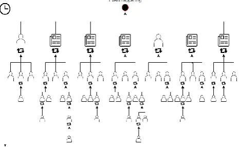
Real news is based on an event that actually happened, whereas false news is based on something that probably did not. This is where the difference in the spreading patterns starts. As there is an intense culture of competition between news firms, it is a race of who brings the news first. This refers back to the statement that novel news is more sharing-worthy. Therefore, if an event occurs, many firms or users will broadcast the news in a short timeframe. Then the news will be talked about and shared on social media, giving a news item a lot of attention when it just shortly has been released. However, as time pursues, the subject will slowly fall into oblivion, up to the point that people barely mention it again. This is called ‘Broadcast dynamics’ [12]. A visual representation of this process is given in figure 1. If an event did not occur, but some individuals pretend it did, we get a different type of diffusion. It won’t get noticed right-away by commercial organizations that benefit financially from broadcasting news. Instead, some users online will notice the news and, because of certain incentives we found earlier in this study, will think the news is worth to show their followers. Some of those users will think the same of the news item, and share it in their turn. This makes that diffusion works its way through the many users who feel like sharing it. This way the rumour gets spread more and more broadly and is referred to as a peer-to-peer diffusion (visualized in figure 2). Vosoughi [12] found that falsehood indeed diffuses in this way. This is an interesting finding, which definitely should be used in the targeting of fake

news. Takahashi et al. [15] made a conclusion that enforces the theory of peer-to-peer diffusion. It was found that overall false rumours were spread by many different users, rather than having a few users spreading it repeatedly.

This peer-to-peer sharing makes that a rumour spreads increasingly fast, as found by Vosoghi et al [12] and Friggeri et al. [11]. It is said that a fake news item on Twitter reached 1500 users six times as fast than a true news item would do [12]. This makes false news more probable to go viral on the internet, as the fake news Tweets cascaded deeper than real news does [11].

2.6.2

Recurrence

Shin et al. [14] researched whether fake news items returned at a later time. The first finding was that real news did not. Once a news item was put online, it never really came back as an actively bespoken subject, even though someone might mention it sometime again. Also found here, was that of the total amount of Tweets on a real news item, half of the Tweets were posted on the most active day.

Fake news, however, did return several times, on average 2.3 times. The most interesting finding that Shin did here, is that for 7 out of 11 Tweets that recurred, the major source was different for each recurrence. This could mean that a new source tried to revive the story, often acting as if it was novel news.

A finding that relates to the Broadcast Dynamics versus Peer-To-Peer Diffusion theory is the ratio of the highest peak to the total Tweets sent about a single item. Real news had as highest spike on average approximately 50 percent of the total Tweets, which is explained by an item being broadcasted at once, to disappear later on. False news however, had an average highest-spike-to-total ratio of just near 20 percent.

2.6.3

Corrections

It is already known that fake news spreads quickly, way faster than real news. But, there is also some positive information in this paragraph: researchers found that correction Tweets spread even twice as fast as the corresponding fake new Tweet [15]. Correction Tweets are Tweets send by users that tell about a fake news story that it is not true, indicating what about the story is false. Even though the sample these researchers used only included two sets of Tweets on two separate stories, it is good news for the battle on fake news. That these corrections spread faster than the original Tweets could be explained by the statement that people don’t share fake news willingly. This is also seen on Twitter, as many of the fake news samples we analysed included users that mentioned or retweeted Snopes repeatedly, a fact-checking organisation with as main mission telling what news is true and what not. This is useful for the tool we are to design, as the datasets of Tweets can be analysed on the occurrences of Snopes articles.

4

3.

THE MODEL

We can now design the model, but before we do so we need to keep in mind that we should comply with a few criteria. The most important criterium is that the model can in no way be biased, the credibility score we aim to produce, should rely on factual and statistical figures only. We should not mainly tell the users what is fake and what is real, this is sensitive to propaganda and biases. We most importantly don’t want to have others tell what is real and what not, this should avoided at all costs. We should provide the users the tools to make their decision in determining what to believe and what not to.

Another criterium is that the model should be implementable by software designers, it should be easily explainable and transformable into code. Therefore we need to address every single step to be taken in the visualisation of the model, and determine how the score will be reflected from the analyses made of the Tweets.

Finally, we should make sure that the output made by the program is easily understandable for every user. As one of our criteria is that the model should not directly tell whether some message is fake or real, we should not just report the findings of the analyses, but give the user the space to tell truth apart from falsity themselves.

Designing our model starts with defining the means we will need for this system to work. We then identify the computations the system will have to do in order to come up with supportive information and prepared data for the credibility scores. Then, based on these defined computations, we specify the calculations that the system will have to perform. The difference between “computation” and “calculation” in this section is defined as such: computations are the steps required to gain the needed figures that will be used by the system in order to perform the calculations; the steps required to come to a credibility score. Finally, we take all the pieces we identified, and put them into one final model.

3.1

Means

3.1.1

Data samples

Diffusion of fake news is our most important overarching factor, as found by our literature research. Fake news has a more forceful way of spreading, misleading its victims and using them to reach more people. In order to analyse the diffusion, we need the bigger picture: as many Tweets about the same subject as possible. This ‘bigger picture’ will also be used to compute the averages of the user-related variables (e.g. number of followers, time on Twitter, etc.).

In order to come with conclusions whether a set of Tweets indicate a real or a false news story, we need to compare the analyses that the model will perform with a large training set. This training set should include a corpus of Tweet sets that already have been labelled as true or false. That means that this training set should exist of Tweet sets that all imply one news item, either true or false. These sets of Tweets will provide the system with all the averages and confident intervals to use for the credibility score calculation.

3.1.2

Twitter JSON Objects

The datasets this model uses are populated by Tweet-objects delivered by the Twitter API or by a commercial organisation that delivers Twitter data. Tweet-objects are delivered in JSON format, a simple way of storing data and communicating data

2 https://developer.Twitter.com/en/docs/Tweets/data-dictionary/overview/Tweet-object.html

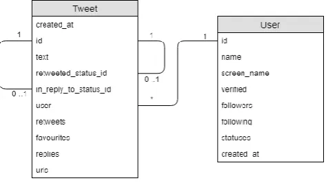
between systems. JSON Objects are designed in a way, which makes it possible to call properties of an object, in this case the Tweet. The Tweet-object in JSON format can be converted to a simple database schema that makes it easy to store all Tweets in a database. In figure 3 we see the Tweet-object represented as a database scheme. Every Tweet has a user, this value can not be empty, and refers to the table that is filled with user data. The relationship between user and Tweet is represented by the line: one user has no, one or multiple Tweets (indicated by the asterisk). A Tweet can be a retweet (Tweet A is a retweet of Tweet B), a reply (Tweet A is a reply to Tweet B) or a standalone Tweet (neither a retweet nor reply). The relationship between Tweets A and B is reflected in the retweeted_Status_id and the

in_reply_to_status_id: one Tweet is a retweet of no or one Tweet, and one Tweet is a reply to no or one Tweet. It should be stated here that these relationships can not exist at the same time, a Tweet is not a reply and a retweet at the same time. The documentation about Tweet objects is found in the API documentation of Twitter2_.

3.2

Computations

After concluding our literary research, we have a considerate amount of variables that we will use when creating the model. These factors will be analysed through four computations:

• Diffusion pattern o Cascades o Tweet density

• Social profiles

o Emotion profile o Global user profile

In the next sections we will explain for each computation what will be computed, why it will be computed and what the outcomes are used for.

3.2.1

Diffusion pattern

Diffusion will be the main focus in our model, as we found characteristics of diffusion that are feasibly measurable through calculations. The differences in diffusion are characterized by five elements:

• number of cascades

• cascade size

• cascade depth

• highest-peak-to-total ratio

• recurrences

5

3.2.1.1

Cascades

With “cascades” we take over the definition of Vosoughi et al. [12]: if users A and B Tweet a Tweet about the same subject independently, therefore not related to each other, that is they are not retweet of or replies to one another, we have two cascades. These Tweets can be retweeted, making the size of the cascade

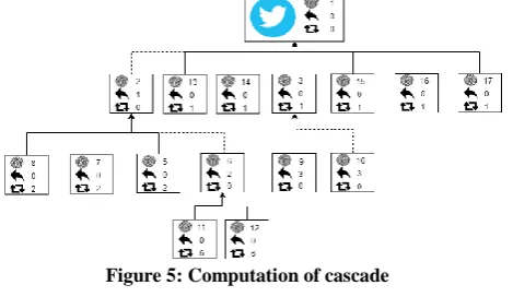
larger. The Tweet can also get replies, also making the cascade larger, and these replies can then again get retweeted. An example of a cascade is given in figure 4. The blue Tweet is the independent Tweet, the dotted lines imply replies and the other lines are retweets. This particular cascade has size 15, we can verify this by counting all the nodes.

We found in our literature research that fake news is reflected by a peer-to-peer diffusion that is sensitive to going viral. In contrast, real news with its broadcast dynamics shows less virality, but more initial sources. If we take the view of the cascades solely at this point, the model can make conclusions about the spreading pattern of a dataset by counting the number of cascades and the size of the cascades. Peer-to-peer diffusion consists of few initial sources and a high virality factor. These initial sources are all independent Tweets, however, not all independent Tweets will be initial sources. We could take only cascades into account that are sent within a certain timeframe, filtering out only initial sources, but then we would discard our finding that fake news might recur. Therefore, counting the cascades will do the trick, as Vosoughi et al. found: the majority of fake news datasets experienced under 1000 cascades, whereas the majority of real news datasets experienced between 1000 and 100000 cascades [12]. The virality factor can be measured by how many people are reached on average in each cascade. Viral news stories reach more people, resulting in bigger cascades. If we take the average of the cascade size, we can compare this to our training dataset, giving us an indication of the size of the virality factor.

Computing the cascades in a set of Tweets is made possible by the data provided in a Tweet JSON object. A cascade starts with an independent Tweet, being a standalone Tweet. All Tweets have IDs that are unique, and make it possible to connect them to one another. So, we first select all independent Tweets. Then we take all Tweets that are replies and retweets, and take the

retweeted_status_id and the in_reply_to_status_id to connect them to one another. This is visualized in figure 5, which shows the same cascade as in figure 4. The blue Tweet has ID 1 and no

3 http://saifmohammad.com/WebPages/NRC-Emotion-Lexicon.htm

4_{https://www.ibm.com/watson/services/tone-analyzer/}

retweeted_status_id nor in_reply_to_status_id. The dashed lines, again, show replies whereas the solid lines show retweets.

3.2.1.2

Tweet density

Tweet density is the unit we use to analyse peaks of high Twitter activity in the Tweet set. To compute the Tweet densities, we first need to create a timeline of Tweets. Each Tweet has a timestamp that allows the model to sort all Tweets on date. Then, we take the timeline and split it into parts, or intervals. Within each interval we count all the Tweets within that hiatus, giving us a set of Tweet-densities. If we plot all these densities in a graph, we can add more credibility to the findings we did in our cascade analysis. Real news broadcasts in a short timeframe, giving a high highest-peak-to-total ratio of approximately 50 percent. We can calculate this by taking the interval with the highest number of Tweet, and dividing these Tweets by the total amount of Tweets.

For the sake of recurrences, we take intervals of one week. This gives us indications whether a story recurred after at least one week of (little) inactivity. Shin et al. proposed to take only peaks into account that are at least 10 percent of the highest peak. Then, of these peaks they set the criterium that the peaks should at least be one week apart from each other [14]. After applying these requirements, we can count the number of occurrences of the story to analyse.

3.2.2

Social profiles

Besides the pattern characteristics, we also found some other useful information regarding fake news data. These two factors belong in the social scope of the statistics and require less effort or steps to compute.

3.2.2.1

Emotion profile

As we found that initiators design their rumours in a way that inspires surprise and disgust from their victims, we can connect these findings to statistical data. By taking the text of every single Tweet, we can use a tone analysis on them. This is done by marking all words with an emotional load. The National Research Counsil Canada released a large dictionary of words with the emotional loads connected to them3_{. These words can} be used to classify the Tweets on emotion and attach a score to them. There also exist tools that are designed for this purpose, for example the IBM tone analyser4 _{or the IBM Watson natural} language understanding5_.

3.2.2.2

Global user profile

As is the case with the emotional level, the analysis of the users will also provide us with a set of numeric variables that will be compared directly with the training data. These variables are quite straightforward to compute, it takes just taking the means of the dataset and comparing this to the found global values. The five figures that are computed here are the significant values Vosoughi et al. found (section 2.2.1).

3.2.3

Supportive information

We found that our model should not be designed to tell users what is true and what not. It should be a supportive tool that helps users decide whether they believe and share something. We found that the core of the problem can be addressed as well, an important finding. If one can tackle, or at least reduce the impact of, the cores of the problem, it would have a great impact in the spread of fake news. The problem lays in the fact that people are

5 https://www.ibm.com/watson/services/natural-language-understanding/

Figure 4: Cascade

6 too naïve; they believe what they see on the internet too easily and don’t see the importance of information triangulation (i.e. an extensive check validating information). This makes that false news propagates easily, and knowing that the speed of diffusion of fake news increases incrementally this has enormous effects. If our model can reduce the effect of the start of the problem, the effects of this way of problem solving will be increasingly large as well, as we try to eliminate early nodes.

3.2.3.1

Partisanship

Concerning partisanship, we found that people tend to believe fake news in favour of their party rather than real news contra their beliefs. We stated that Wijnhoven & Brinkhuis [5] found that the opinions of participants in a test were influenced more by non-expert views than information triangulation. We can use this in our model, by giving the users an overview of opposing Tweets: a clear list of negative Tweets, next to a list of positive Tweets. In order to achieve this, all Tweets need to be analyzed on sentiment. The process of attaching a sentiment score to a Tweet could either be done by creating an own algorithm, or by using an existing API. The IBM Watson natural language understanding tool mentioned earlier5 _{gives a score of sentiment} given a text as input.

3.2.3.2

Sources

Part of the lack of analytical thinking from the subjects in case, involves source checking. Subjects fall for messages even though the sources don’t seem credible [14]. We already explained that we can’t put the words in the mouths of Twitter users, we have to let them resolve the integrity of the sources. If a person is subject to one particular fake news message that is included, they have to decide whether they believe the story based on one source. We could simply list all the sources found in the Tweets, as the Tweet-object provides a property for included sources (Figure 3). Then, we could group all Tweets on included source, making us able to count how often a source is used.

Using an effortless text analysis we can also let the system detect whether Snopes articles are found corresponding the subject. This just involves checking whether Snopes is mentioned in the Tweet set the model analyses. This could give the users an easy way to fact-check the articles addressed by Snopes.

3.3

Calculations

All the computations result in a set of variables to be verified, weighted and converted into a score. The output variables given by the computations represent the two categories: diffusion pattern and social profiles. To come to a final score we first need to score these sets separately.

3.3.1

Comparing value to mean

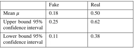
We want to score the variables on a scale of 0 to 1, with 0 probably fake, and 1 probably real. The training set consists of data that is classified into two classes, real and fake. These classes have for all the variables that are computed a mean and a confidence interval. We want to compare the test variable to both classes to see to which it corresponds the most. This method will work for all variables, but we use the highest-peak-to-total ratio as an example. Let’s say our training sample came with these figures:

Table 1: Dummy figures as example

We take as an example a test figure of 𝜇 = 0.26. We want to find where between these classes our test figure lays. For this we need to take the 95%-confidence interval into account, as one sample probably will have more data records 𝑛. When our test variable is 18 it is probably fake, and when its 50 it is probably real. First we need to plot a graph of the differences in numbers, where our test variable is defined as 𝑥.

𝑦 = ((𝑥 − 0.18) + (𝑥 − 0.25) + (𝑥 − 0.11))

+ ((0.50 − 𝑥) + (0.62 − 𝑥) + (0.38 − 𝑥)) = 6𝑥 − 2.04

Then we need to find 𝑦 = 0, as a difference of 0 lays exactly in between the means. This is when we can’t really say much about the class, thus giving a score of 0.5. In this example, 𝑦 = 0 → 𝑥 = 0.34. Now we need to find the extreme values, these are the points from which we say the score is either 0 or 1. As we have the confidence level of 95% for all the values, we can take the lower value of 𝑥 = 0.11 → 𝑦 = −1.38 and the upper value of

𝑥 = 0.62 → 𝑦 = 1.68, this gives us a range of (-1.38, 1.68) with size 1.68 − −1.38 = 3.06 and a midpoint of 0.15. From these points the score will be 0 or 1 respectively. Our test variable yields in a difference of 𝑦 = −0.48. As we take 0 as our midpoint, we should apply a correction the outcome: −.48 + .15 = −0.33. This tends slightly to the fake class with a score of

|−1.38−−0.33| 3.06 = 0.34.

We can form these calculations into a generic set of formulas:

𝑦 = 6𝑥 − 𝜇𝑓𝑎𝑙𝑠𝑒− 𝐶𝐼𝑙𝑜𝑤−𝑓𝑎𝑙𝑠𝑒− 𝐶𝐼ℎ𝑖𝑔ℎ−𝑓𝑎𝑙𝑠𝑒− 𝜇𝑡𝑟𝑢𝑒− 𝐶𝐼𝑙𝑜𝑤−𝑡𝑟𝑢𝑒

− 𝐶𝐼ℎ𝑖𝑔ℎ−𝑡𝑟𝑢𝑒

𝑚𝑖𝑛 = min (𝐶𝐼𝑙𝑜𝑤−𝑓𝑎𝑙𝑠𝑒, 𝐶𝐼𝑙𝑜𝑤−𝑡𝑟𝑢𝑒)

𝑚𝑎𝑥 = max (𝐶𝐼ℎ𝑖𝑔ℎ−𝑓𝑎𝑙𝑠𝑒, 𝐶𝐼ℎ𝑖𝑔ℎ−𝑡𝑟𝑢𝑒)

𝑟 = (𝑦𝑚𝑖𝑛, 𝑦𝑚𝑎𝑥)

𝑑 = 𝑦𝑚𝑎𝑥− 𝑦𝑚𝑖𝑛

𝑚 = 𝑦𝑚𝑖𝑛+

𝑑 2

𝑆 = 𝑖𝑓 (𝐶𝐼𝑙𝑜𝑤−𝑓𝑎𝑙𝑠𝑒< 𝐶𝐼𝑙𝑜𝑤−𝑡𝑟𝑢𝑒) 𝑡ℎ𝑒𝑛:

|𝑦𝑚𝑖𝑛− (𝑦𝜇𝑡𝑒𝑠𝑡+ 𝑚)|

𝑑 , 𝑒𝑙𝑠𝑒:

1 −|𝑦𝑚𝑖𝑛− (𝑦𝜇𝑡𝑒𝑠𝑡+ 𝑚)|

𝑑

Where 𝑦 is the aggregate difference of 𝑥, 𝑚𝑖𝑛 is the lowest value of the 95%-Confidence Intervals, 𝑚𝑎𝑥 is the highest value of the 95%-Confidence Intervals, 𝑑 is the size of range 𝑟, m is the midpoint applied for correction, and S is the score we are calculating.

3.3.2

Score weights

It is desirable that all scores are applied to a weight that suits the significance of the score. However, to say what weight fit what score to be as accurate as possible, we need more research on this. Therefore, in our model we consider all the factors of the output variables equal. The final score of one output will be done by averaging out all the sub-scores.

What we do know, however, is that diffusion should weigh heavier than the social aspect of the model. It is impossible at this point to research which weights are appropriate here, so we will define the weight as 𝑘. We will multiply the output-score of the social aspect with 𝑘 and the output-score of the diffusion aspect with 1 − 𝑘. Finding out what 𝑘 works best is done by testing the model once it is programmed.

Fake Real

Mean 𝜇 0.18 0.50

Upper bound 95% confidence interval

0.25 0.62

Lower bound 95% confidence interval

7

3.4

Final model

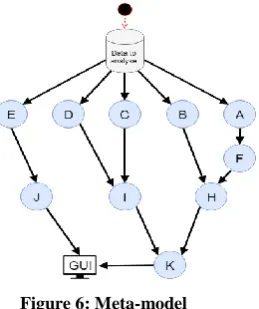
Our vision on how the model should look like is pretty clear at this point. We are now set to merge all puzzle pieces into one streamlined application. In order to complete this puzzle, we first need a clear overview of what pieces we have, in our case the steps that need to be taken. As the training dataset will have to be prepared only once, we don’t consider this as a task in our model. The training of this data is similar to the calculations we apply to the dataset to analyse. The final model is visually worked out in a meta-model (Figure 6) and in detail in Appendix 1.

3.4.1

Meta-model

Our model starts when a dataset to analyse is inserted. Then, the system will perform five parallel computations (A-F, B, C, D and E), all needed to get to the output variables we need (H, I and J). A-F computes the Tweet density, B is the computation of the cascades, C is the computation of the emotion profile, in D the user profile is generated and E groups the Tweets on source and sentiment for supportive information. Two output variables (H and I) are used for statistical tests and score calculation (K) and the other (J) is used for supportive purposes. In the score calculation the trained dataset is used to compare all found figures with. All of these tasks follow their own route to the Graphical User Interface, where the data is presented in an understandable way.

3.4.2

Example for the model

The full version of the model (Appendix 7.1) is filled with explanatory dummy data. The figures contained in the model are used for the explanation given for this example. It starts when the system is given the task to perform the analysis on the Tweet set on one similar news item. Then the five parallel tasks start. We will follow the different paths to the GUI.

Table 2: Tweet densities

One task is to sort all Tweets on date and split it up into parts (A). These intervals are used to plot a density over time graph (F). The Tweet symbols in 7.1A indicate approximately 1000 Tweets. The (example) figures that belong to the Tweet density computations are given in table 2 (and in the graph of 7.1F). This table shows the week number, the Tweet-density, the ratio of density-to-highest-peak and the accumulative percentages of the densities. We see that the highest density is 14.8 percent, this gives us a highest-peak-to-total ratio of 0.148. Week 8 and week 11 (made red) have a density-to-highest-peak ratio of less than

10 percent, giving us two gaps in the sample. Therefore, the story of this sample occurred three times (also seen in 7.1H). The second parallel task is computing the cascades in the way we explained in 3.2.1.1. From these computations we can count the number of cascades, the largest cascade size and the average cascade size. Tasks A-F and B result in a table of output variables (H).

The third and fourth task (C and D) are on the social scope of the analysis. These are fairly straightforward computations as

described in 3.2.2. The outcomes of these computations are stored in the output variables I.

The fifth task involves grouping the Tweets on source and sentiment. These outputs, stored in the output variables J, are used for the supportive tools of the model. These outputs won’t be scored or compared, but will give an overview to the user in the GUI.

The output variables of H and I will be used to score the credibility in the score calculation K. In appendix 7.2 and 7.3 we see the tables with all the dummy data we use in this example (table 3 and table 4). The figures we want to test to find a credibility score (i.e. the figures from 7.1H and 7.1I) are written down in the column “Found test value”. The other values in the “False” and “Real” classes are demo figures of the values the model would use to calculate the credibility-score. These values are approximations of what the numbers would be using a training set of data. These approximations are based on our findings in the literature, and some are based on a small set of Tweets we selected ourselves. This set of Tweets consists of 12 stories that are indicated as false by Snopes and 8 stories that are selected on credible news sites (e.g. BBCNews). The set contains in total 1807 Tweets on the false topics and 1038 Tweets on the true topics.

The scores are calculated using the formulas of section 3.3.1. In total, the numbers result in a diffusion pattern of 0.27, with 0 being peer-to-peer diffusion and 1 being broadcast dynamics, and in a social profile score of 0.38, with 0 being fake and 1 being real. If, for example, we found in further research a k value of 0.3, the model would return a final credibility score of (0.7*0.27)+(0.3*0.38)=0.30, indicating that the set of Tweets might concern fake news.

3.4.3

GUI

The GUI is the only thing that forms the bridge between the system and the user. The user interacts with the GUI, the GUI translates this to the system that performs calculations and returns an output, which then again is shown to the user. As we have quite a lot of information stored in the output variables, we can provide the user with a lot of information. Though, this is not desirable, since we specified that “[…] that the output made by the program is easily understandable by every user” (section 3). We should only give what all users can understand easily, which means the system shouldn’t overthrow the user with knowledge. The main information that should be provided is:

• Occurrence of Snopes (and if so, a link to the article)

• Opposing Tweets (sorted on most extreme value, descending)

• The credibility score

• Explanation of the diffusion pattern

Week Density % Acc

1 0.053 0.36 0.053

2 0.148 1.00 0.201

3 0.072 0.48 0.273

4 0.080 0.54 0.353

5 0.096 0.65 0.449

6 0.081 0.54 0.530

7 0.042 0.28 0.572

8 0.008 0.05 0.580

9 0.041 0.28 0.621

10 0.020 0.13 0.641

11 0.006 0.04 0.647

12 0.047 0.32 0.694

13 0.054 0.37 0.748

14 0.095 0.64 0.843

15 0.103 0.69 0.946

16 0.055 0.37 1.000

8

4.

CONCLUSION

After a journey through the universe of fake news, we can concretely answer our research questions. R1 asked how it is possible that fake news has this much success. In section 2.1 we addressed this problem. We found that humans are sensitive and reactive to stimuli and emotion. Add to this that many people falling for fake news lack the ability to think analytical, or at least refuse to do so out of carelessness, we see that people are quite naïve. Partisanship is also showed to be a root cause of the success of fake news, a factor that is gladly used by initiators. Stating in R2, we wanted to find out what would set fake news apart from real news. The focus before the literature research was mainly on fact-checking as a solution to fake news, however, we found a characteristic that completely changed the scope of the research. It seemed that diffusion is the most obvious part that sets fake news apart from real news, this also seemed very well explainable. Besides diffusion we found that some other characteristics were different for fake news, like the user profiles of the users involved in the spreading. All the factors we found in this paper, also shifted the focus from both an individual Tweet and the set of Tweets on the same subject, to just the large set of Tweets on the same subject. This is due to the most valuable information being taken from the ‘bigger picture’, and individual Tweets need more research still.

5.

FURTHER RESEARCH

I have found a few points of attention in further research. Vosoughi et al. found a few good points regarding cascades. However, it is thinkable that real news items that are not very popular will have less cascades, and therefore might be mistaken for fake news on this factor. On the other hand, popular news might have great virality, and therefore might also be mistaken. It could be a good to do some research on the relationship between the number of cascades and the size of the cascades. We mentioned an undefined variable 𝑘 in the model, research should be done on what the best fitting figure is, making the model as accurate as possible. Besides this weight, we did not apply any other weights to the scores, it would be good if these scores can be tweaked using weights as well, resulting in better calculations.

Finally, our model is just a design, it is not functional yet. If such a system would be programmed into a functional system, it enables more room to test it on accuracy, or on the effects on users. This testing also enables the ability to tweak the system by trial and error, making it better and better.

6.

REFERENCES

[1] Miriam J. Metzger and Andrew J. Flanagin. 2013. Credibility and trust of information in online environments: The use of cognitive heuristics. (September 2013). https://www.sciencedirect.com/science/article/pii/S0378216613 001768

[2] Hunt Allcott and Matthew Gentzkow. 2017. Social Media and Fake News in the 2016 Election. (2017). https://nyuscholars.nyu.edu/en/publications/social-media-andfake-news-in-the-2016-election

[3] Philip Fernbach, Todd Rogers, Craig Fox, and Steven Sloman. 2012. Political Extremism is Supported by an Illusion of

Understanding. PsycEXTRA Dataset(2012). DOI: http://dx.doi.org/10.1037/e519682015-069

[4] Gordon Pennycook, Tyrone D. Cannon, and David G. Rand. 2017. Prior Exposure Increases Perceived Accuracy of Fake News. SSRN Electronic Journal(2017). DOI: http://dx.doi.org/10.2139/ssrn.2958246

[5] Fons Wijnhoven and Michel Brinkhuis. 2014. Internet information triangulation: Design theory and prototype evaluation. Journal of the Association for Information Science and Technology 66, 4 (February 2014), 684–701. DOI: http://dx.doi.org/10.1002/asi.23203

[6] B.E. Weeks and R.K. Garrett. 2014. Electoral Consequences of Political Rumors: Motivated Reasoning, Candidate Rumors, and Vote Choice during the 2008 U.S. Presidential Election. International Journal of Public Opinion Research26, 4 (May 2014), 401–422. DOI: http://dx.doi.org/10.1093/ijpor/edu00 [7] S. Mo Jang et al.2018. A computational approach for examining the roots and spreading patterns of fake news: Evolution tree analysis. Computers in Human Behavior84

(2018), 103–113. DOI:

http://dx.doi.org/10.1016/j.chb.2018.02.032

[8] L. Itti and P. Baldi. 2009. Bayesian surprise attracts human attention. Vision res(2009), 1295–1306.

[9] A. Friggeri, L. Adamic, D. Eckles, and J. Cheng. 2014. Rumor cascades. Proceedings of the Eighth International AAAI Conference on Weblogs and Social Media(2014), 101–110. [10] Niall J. Conroy, Victoria L. Rubin, and Yimin Chen. 2015. Automatic deception detection: Methods for finding fake news. Proceedings of the Association for Information Science

and Technology52, 1 (2015), 1–4. DOI:

http://dx.doi.org/10.1002/pra2.2015.145052010082

[11] Dongsong Zhang, Lina Zhou, Juan Luo Kehoe, and Isil Yakut Kilic. 2016. What Online Reviewer Behaviors Really Matter? Effects of Verbal and Nonverbal Behaviors on Detection of Fake Online Reviews. Journal of Management Information

Systems33, 2 (February 2016), 456–481. DOI:

http://dx.doi.org/10.1080/07421222.2016.1205907

[12] S. Vosoughi, D. Roy, and S. Aral. 2018. The spread of true and false news online. Social Science359, 6380 (2018), 1146– 1151. DOI:http://dx.doi.org/10.1126/science.aap9559

[13] Yuko Tanaka, Yasuaki Sakamoto, and Hidehito Honda. 2014. The Impact of Posting URLs in Disaster-Related Tweets on Rumor Spreading Behavior. 2014 47th Hawaii International

Conference on System Sciences(2014). DOI:

http://dx.doi.org/10.1109/hicss.2014.72

9

7.

APPENDIX

10

7.2

Table 3: Output variables H (approximations based on theory) Variable Found

test value

Found training figures Score

Fake Real

CI-low 𝜇 CI-hi CI-low 𝜇 CI-hi

Highest-peak-to-total ratio

0.148 0.11 0.18 0.25 0.32 0.50 0.68 0.16

Total peaks 3 3.09 3.31 3.40 0.69 1.00 1.31 0.18

Number of

cascades

400 327 610 893 10415 51140 91865 0.22

Average cascade size

4.78 1.58 2.05 2.52 0.40 1.53 2.66 0.00

Greatest cascade 1512 4899 21503 38107 13 1217 2421 0.77

7.3

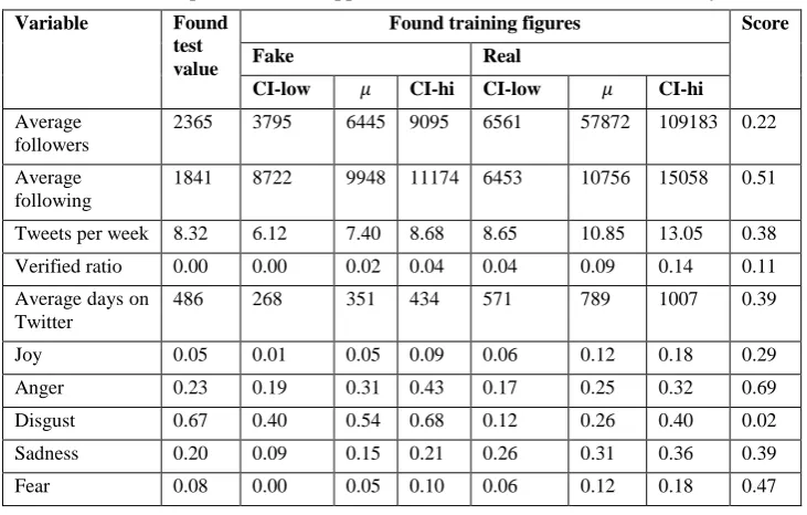
Table 4: Output variables I (approximations based on Tweet set and theory) Variable Found

test value

Found training figures Score

Fake Real

CI-low 𝜇 CI-hi CI-low 𝜇 CI-hi

Average followers

2365 3795 6445 9095 6561 57872 109183 0.22

Average following

1841 8722 9948 11174 6453 10756 15058 0.51

Tweets per week 8.32 6.12 7.40 8.68 8.65 10.85 13.05 0.38

Verified ratio 0.00 0.00 0.02 0.04 0.04 0.09 0.14 0.11

Average days on Twitter

486 268 351 434 571 789 1007 0.39

Joy 0.05 0.01 0.05 0.09 0.06 0.12 0.18 0.29

Anger 0.23 0.19 0.31 0.43 0.17 0.25 0.32 0.69

Disgust 0.67 0.40 0.54 0.68 0.12 0.26 0.40 0.02

Sadness 0.20 0.09 0.15 0.21 0.26 0.31 0.36 0.39