Activity classification through hidden Markov modeling

(1)

MASTER THESIS

Activity Classification through

Hidden Markov Modeling

Thijs Tromper March 1, 2016

Faculty of EEMCS

Department of Applied Mathematics Chair Applied Analysis

(2)

(3)

Abstract

The goal of this study is to improve upon an existing activity classifier software model called FusionAAC, previously developed at Roessingh Research and Development. FusionAAC applies a technique called Hidden Markov Modeling to automatically and independently classify human activities. It mainly uses kinematic motion sen-sor data as input, but other input data types are also possible. The FusionAAC software is based upon the Hidden Markov Toolkit 3.4, implemented in a Labview environment.

(4)

(5)

Preface

This report covers my combined internship and master’s research project, carried out towards receiving a master’s degree in Applied Mathematics at the University of Twente. The main body of work was done at Roessingh Research and Develop-ment (RRD) in Enschede. I would like to thank my daily supervisor Chris Baten for putting his trust in me and giving me the opportunity to put my theoretical knowledge to practical use. I would further like to thank Leonie for her invaluable input which greatly helped me translate our research questions into mathematics.

(6)

(7)

List of symbols

HMMs

Symbol Description

t Clock time

T Total number of clock times, 1≤t≤T

S State space of a Markov chain

N Total number of states in a Markov chain qi State iin a Markov chain, 1≤i≤N Xt State of a Markov chain at clock time t

X Markov chain state sequence X1· · ·XT π

ππ Initial state probability distribution of a Markov chain, see (2.3) A Transition probability matrix {aij}of a Markov chain, see (2.1)

V Space of observable signals

M Total number of distinct observable signals vk Discrete observable signal k, 1≤k≤M Ot Observable signal at clock time t

O Sequence of observations O1· · ·OT

Ot1:t2 _{Sequence of observations from time} _t1 _to_t2: _O

t1· · ·Ot2

B Vector of observable signal distributions {bj(·)}, see (2.2) λ Compact notation for a HMM, λ= (A,B, πππ)

αt(j) Forward variable, see (2.5) βt(j) Backward variable, see (2.6)

γt(j) Probability state qj at timet, see (2.8)

δt(j) Probability partial best path ending at stateqj at timet, see (2.11) Ψt(j) Most likely state qj at time tin partial best path, see (2.12)

ξt(i, j) Probability of state qi at timetand stateqj at time t+ 1, see (2.13)

HTK

Symbol Description S Substitution error

(12)

Acronyms Meaning

HMM Hidden Markov Model

MLE Maximum-Likelihood Estimation

DMD Duchenne Muscular Dystrophy

AT Assistive Technology

ADL Activities of Daily Life

HTK Hidden Markov model Toolkit

TV Total Variation

MAP Maximum A-posteriori Probability

Formulas Description and use

P(A|B) = P(A, B)

(13)

Chapter 1

Introduction

1.1 Background

Over the past two decades, inertial sensing technology has seen considerable improve-ment. Accelerometers and gyroscopes have not only become much more accurate, it is now also possible to build cheap, highly miniaturized sensors. These developments give rise to a wealth of new research fields where motion sensing can be applied.

One of these fields is rehabilitation technology. In rehabilitation, a therapist often needs some way to quantify function and progress of a patient. To this end, it is important for the therapist to be able to observe patients in a setting that comes as close to their natural environment as possible, while at the same time the observation is as objective and accurate as possible. For example, it is better to observe patients walking normally compared to them walking on a treadmill, but it might be easier to quantify motion on a treadmill. Some rehabilitation therapists might have access to a motion analysis laboratory, but this is still not ideal. The walking space in laboratories usually is no more than ten meters, which makes it difficult to measure more than two gait strides in their entirety. On top of this, the setting (artificial floor, pressure to perform) is far from optimal. In other words, to make it easier to provide the best possible care, it would be much better to be able to observe patients accurately and objectively during normal daily life.

This is where modern sensors come into play. The new generation of inertial sen-sors show great potential to measure patients during normal daily life. Lightweight, easy to position sensors, that are easily worn underneath clothing, are becoming the standard. Not only are these sensors not affecting the wearer’s ability to perform normal daily activities, the possibility to wear them underneath clothing greatly in-creases social acceptance. The challenge now is to achieve the same level of accuracy that is obtained in a laboratory setting.

(14)

being analyzed. Typically, existing automated activity recognizers are only able to distinguish a few general activities. In practice this means that any recorded data has to be manually annotated to make sure it is interpretable at a later time. These constraints make data acquisition enormously time-consuming. And so there arises huge potential for accurate automated activity classification.

1.2 Activity classifiers

What is needed is an activity classifier that can distinguish between a series of activities that are very specific to for example rehabilitation exercises of a patient, or the job of a worker being analyzed. Moreover, after some initial learning process, the classifier is able to do this independently and automatically.

The sensor solution that provides the data for the classifier needs to be as ’mini-mal’ as possible. That is, it needs to be lightweight so as to not affect the activities it tries to measure. It should consist of as few sensors as possible, positioned on the body in the least cumbersome locations, while at the same time it still provides enough data to capture the essence of any activities of interest.

1.2.1 Prior research

Over the past decade Roessingh Research and Development [26] (henceforth RRD) has been working on both ambulatory sensing solutions and activity classification. The work on ambulatory sensing resulted in the Fusion project (2009-2013) [2], where among other things the positioning and calibration of motion sensors on the human body was researched. The project culminated in the development of tools to accurately and objectively monitor motor function in physical and rehabilitation therapy, and sports. These tools were used to monitor the influence of fatigue on the coordination of subjects running a marathon, and to provide rowing coaches with comprehensive, accurate information about the movement, timing and behavior of competitive rowers.

(15)

1.2.2 Goals

After the initial groundwork done by RRD, some fundamental questions now have to be addressed. Maybe the most important part of designing an activity classifier is the training process. Without the right training, it will never be capable of high accuracy recognition. It is vital to assess whether a training set not only contains enough information, but also the right kind of data to effectively train the model. One of the main challenges addressed in this research will therefore be generalizing and optimizing the training effort. Some other aspects we will go into are:

• Data preprocessing: making sure that the amount of information in the data is maximized, while the amount of noise is minimized.

• The ability of the classifier to deal with classification (in)securities, e.g. dealing with classification doubt between multiple activities, most notably dealing with false positives.

• Minimizing the computational load.

1.3 Classifying arm and hand function in Duchenne

pa-tients

Duchenne muscular dystrophy (DMD) is a genetic disorder caused by a mutation in the dystrophin gene. This gene codes for the protein dystrophin, which strengthens muscle cells by attaching parts of the internal cytoskeleton to the cell membrane. Without it, the cell membrane becomes permeable, eventually causing cell burst due to excessive internal pressure. This results in a cycle wherein muscle fibers deteri-orate and regenerate until the repair capacity of the tissue is no longer sufficient. The degeneration of the fibers becomes irreversible and muscle cells are replaced by fat cells and connective tissue.

The dystrophin gene is located on the X chromosome. It is a recessive gene. This means that both sexes can carry the mutation, but mainly male children are affected by DMD. Worldwide, one in 3500 male children [12] suffers from the disease. Only one percent of people with DMD is female. It is the most common inherited muscle disease in children.

(16)

At present, there is no cure for DMD. Treatment is generally aimed at controlling the symptoms to maximize the quality of life. Maintaining upper extremity function is very important in daily life, so physical therapy is vital to help maintain strength and flexibility. Inactivity can worsen the disease. Orthopedic appliances, such as wheelchairs and leg braces, may improve mobility and independence. As the disease progresses, it becomes necessary to support respiratory function.

Over the last couple of decades, new and improved ways of treatment have led to DMD patients living much longer. The average life expectancy for people with DMD currently is 27 years, but because of the individual variation in the progression of the disease, this differs from patient to patient. Nowadays half of the patients live past the age of 30. Some even live into their 40s and 50s. However, quality of life has not increased accordingly.

1.3.1 Adapt project

Loss of upper limb function has a major impact on the quality of life of patients. Many patients (not only those suffering from DMD, but for example also multiple sclerosis patients, or people recovering from a stroke or spinal cord injury) depend on assistive technology (AT) to support them during activities of daily life (ADL) like eating and drinking, reading or working on a laptop. Better assistance for patients means an increased level of independence and social participation, which greatly improves the quality of life. An example of an assistive device could be a wheelchair mounted (dynamic) arm support, see for example [36].

Unfortunately, current AT is not yet sufficiently matched to the capabilities and preferences of patients. This is why many patients stop using the technology [5]. Reasons for this are that users have to change numerous settings to switch between different activities, assistive devices do not know whether a user intends to be active, and the performance of devices only tends to be partially helpful.

With this in mind, the goal of the Adapt project [23] (part of the Symbionics Program [22]) is to research and develop new models and methods for future gener-ations of AT. The project focuses on understanding the mutual interaction between patients and assistive devices. The goal is to provide an optimal physical support for the user and adjust the assistance according to the dynamics of the requirements set by task, user or environment. This personalized approach gives patients a central role in defining requirements and priorities in the development of assistive devices. Devices should continuously (co-)adapt to the user: according to a therapy plan (e.g. increased support when a patient gets tired), to compensate for user changes (e.g. in the case of disease progression), changing environments and changing tasks. Furthermore, the goal is to design assistive devices that completely fit underneath regular clothing, which is important for social acceptance.

(17)

robust sensing solution needs to be developed to monitor the interaction between user and assistive device during activities of daily life. Ultimately, this should lead to an assistive device that is able to recognize and predict in real time what spe-cific activity a user is performing. The device can use this information to optimally support the user.

1.3.2 Role of RRD

The real-time co-adaptive device as described in the previous section is still some-thing for the (hopefully nearby) future. The first step towards such a device is highly accurate activity recognition. RRD plays an important role in this part of the Adapt project. Not only can the existing knowledge on activity classification be applied, there is already some prior experience with the classification of activities of DMD patients (see again [44], part of the Fusion project).

With accurate activity classification it becomes possible to get an idea of the typical daily activities of DMD patients. This knowledge can be used to identify where DMD patients could benefit most from AT. Ultimately, as the activity classi-fier becomes more advanced, it could in theory also be used for real-time recognition and prediction. This last part is beyond the scope of this research.

1.4 Overview of this report

Before we can start describing the modeling process for the classification of human activities, first it is necessary to explain the basics of hidden Markov modeling. Chapter 2 consist of an introduction to the theory of hidden Markov models. Chapter 3 describes the acquisition and processing of the data that will serve as input to the activity classifier. It also describes the process of modeling human activities and the software implementation of the theory from chapter 2, resulting in a working activity classifier.

(18)

(19)

Chapter 2

Hidden Markov models

2.1 Introduction

Hidden Markov Models (henceforth HMMs) were first introduced and studied in the late 1960s and early 1970s by Leonard E. Baum and his coworkers. The technique is especially suitable for the modeling of processes that have a sequential quality, e.g. speech. Such processes typically produce time series with homogeneous zones, where the observed data within these zones are governed by similar distributions. In the case of speech, these zones can be phonemes that are characterized by a certain frequency. Starting from the mid-1970s, speech recognition was one of the first fields where HMMs were successfully applied [15] [24].

After the initial success realized in speech recognition, more research fields fol-lowed. Nowadays HMMs are widely known for their applications in describing or classifying a wide range of processes. Some examples closely related to speech recog-nition are handwriting [7] and sign language recogrecog-nition [32]. The technique has also proven useful in modeling biological processes such DNA sequence analysis [18], au-tomated musical accompaniment of human performers [20] and even computer virus detection [41].

To familiarize the reader with the modeling problem, this chapter will start with a toy example. In section 2.3 we will present a general hidden Markov model and discuss the various parameters of this model. Finally, section 2.4 describes how to estimate these model parameters.

2.2 Toy example

(20)

2.2.1 A hidden coin toss experiment

To understand the concept of HMMs, consider the following situation. Suppose you are in a room that is separated in two by a curtain. On the other side of the curtain, hidden from view, a coin tossing experiment is being performed. Because of the curtain, the exact nature of the experiment is unknown, but at regular time intervals the results are called out to you. A possible sequence of “observations” on your side of the curtain would look like

O=O1O2O3· · ·OT =T HH · · · T

whereH stands for “heads” andT stands for “tails”.

The question now is, how to build a model that best explains the observed sequence of heads and tails? The first problem is deciding which part of the real-world process you want to describe through the hidden Markov chain states, and how many of these states are needed. Secondly, the observable stochastic process needs to be defined.

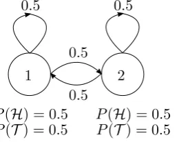
For the purpose of this discussion we will make things a little more interesting and skip the easiest explanation, namely that the person on the other side of the curtain is simply tossing a single coin and calling out the result to you. A simple model for explaining the sequence of coin tosses is given in figure 2.1. We will call it the “2 fair coins” model.

1 2

0.5 0.5

0.5 0.5 P(H) = 0.5 P(T) = 0.5

[image:20.595.239.368.407.510.2]

P(H) = 0.5 P(T) = 0.5 Figure 2.1: “2 fair coin” model

It consists of two states. Each state corresponds to a different coin being tossed. The observable signal in each state is the result of this coin toss, which makes the observable process stochastic. The state transitions between the different coins could in turn be described by another coin toss, independent of the first two. Each face of this third coin is associated with one of the coins corresponding to the states. Note that because of the fairness of all coins, the complete process is statistically no different from a single, completely observable, fair coin toss experiment.

(21)

still no different from a single, completely observable, fair coin toss experiment. The introduction of two different, biased coins does however present us with new possibilities to explain more complex statistical behavior of the observation sequence.

1 2

0.5 0.5

0.5 0.5 P(H) = 0.75 P(T) = 0.25

[image:21.595.214.345.161.260.2]

P(H) = 0.25 P(T) = 0.75 Figure 2.2: “2 biased coins” model

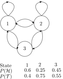
The third and final coin toss example we will present here is called the “3 biased coins” model (figure 2.3). It consists of three states, each corresponding to a different biased coin. The first coin is slightly biased towards “heads”, the second is strongly biased towards “tails”, and the third is slightly biased towards “tails”. In this model, the behavior of the observation sequence depends strongly on the state transition probabilities. Consider for example the cases where the probability of staying in the second state is very large (P22 > 0.95) or very small (P22 < 0.05). Very different long term statistics will arise from these two extremes.

1 2

P(H) P(T)

3

State 1 2 3

0.6 0.4

0.25 0.75

0.45 0.55 Figure 2.3: “3 biased coins” model

[image:21.595.224.357.419.587.2]

(22)

the model is, the more unknown parameters it has. If the observation sequence is too small compared to the number of unknown parameters, it becomes impossible to reliably estimate all these parameters, and any resulting HMMs of different sizes may not be statistically different.

2.2.2 A ball and urn model

To fix ideas, we will extend the ideas presented in the coin toss experiments to a slightly more complicated ball and urn model. Consider the following situation. A room contains a number of urns. Each urn contains a large amount of different colored balls. According to some unknown random process an urn is chosen at regular intervals. When an urn is selected, a ball from this urn is selected. The color of this ball is recorded as the observation and the ball is then replaced in its original urn. The process is repeated until some finite observation sequence of colors is generated.

We would like to model the observation sequence as the observable output of a HMM. A natural choice is to let the number of urns correspond to the states of the hidden Markov chain. The random process through which the urns are chosen is modeled as the transition probability matrix of the Markov chain. The distribution of the observed colors is modeled through a set of discrete observation distributions, one for each urn. The remaining problem then consists of estimating the parameters of both the transition probability matrix and the observation probability distribu-tions.

2.3 A general hidden Markov model

This section will describe the basic elements of a general HMM. All examples treated in the previous section contained a discrete observation process. First we formally define the model notation for such discrete observation HMMs. We will go into the structure of the underlying Markov chain and its implications for the model. Lastly, we will say something about the distribution of the observable signals and extend the model notation to the continuous case.

2.3.1 Definitions and notation

A basic, discrete HMM is characterized by five elements, namely

1. A finite number of unobservable states N. Each state can broadcast an ob-servable signal that possesses some measurable, distinctive properties. The individual states are elements of the state spaceS ={q1, q2, . . . , qN}, and the state at timetis denoted as Xt.

2. The state transition probability matrixA={aij}, where

(23)

That is, a transition to a new state only depends on the current state (the Markov property). Furthermore, the transition probabilities are independent of the time t(the process is stationary). If it is possible to go from one state to another in a single step, we have that aij > 0. Otherwise aij = 0. Note that the rows of the matrix should sum up to one:

N

X

j=1

aij = 1.

3. The number of distinct observable signals M. For the coin toss experiments these signals were simply “heads” and “tails”. For the ball and urn model,M is the total number of distinct colors. The individual signals are denoted as

V ={v1, v2, . . . , vM}, and the signal at time tis denoted as Ot.

4. The distribution of the observable signals in statej,B={bj(k)}, where bj(k) :=P(Ot=vk|Xt=qj), 1≤j≤N, 1≤k≤M. (2.2) Again we assume that the process is stationary, i.e. B is independent of the timet.

5. The initial state distributionπππ={πi}, where

πi :=P(X1 =qi), 1≤i≤N. (2.3) At each clock time 1 < t ≤ T, a new state is entered based upon the transition probability matrix A. This state then generates some observable signal. From the above model, a sequence of these observationsO=O1O2· · ·OT is generated in the following way:

1. Generate an initial stateX1=qi, using the initial state distributionπππ. 2. Sett= 1.

3. GenerateOt=vk, using the distribution of observable signals in stateqi,bi(k). 4. Transit to a new stateXt+1 =qj, using the transition probability matrixA. 5. Sett=t+ 1. If t≤T, return to step 3, otherwise terminate the procedure.

Summarizing, we note that a complete definition of a HMM requires specification of the three probability distributionsA,B andπππ (and implicitly the dimensionsM and N). For the sake of convenience, we will henceforth use the compact notation

(24)

2.3.2 The underlying Markov chain

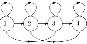
In section 2.2 we discussed some examples of simple HMMs. In all of the underlying Markov chains of these examples every state could be reached in a single step from any other state. A model of this type has the property that all elements of the transition probability matrix Aare strictly positive. These kinds of Markov chains are also called ergodic.

Other architectures are also possible. Here we would like to discuss one particular alternative in more detail, namely the left-to-right model. It is called a left-to-right model because as time increases, the state index does not decrease, i.e. the states proceed from left to right. Architectures like these impose a temporal order to a HMM, since states with a lower index number are linked to observations occurring prior to those that are linked to states with a higher index. For this reason, in speech recognition often left-to-right Markov chains are used [24] [10, p. 33] [6, p. 614].

The transition probability matrix of a left-to-right model has the property that aij = 0, j < i,

i.e. A has an upper triangular form. Furthermore, since the sequence must begin in state 1 the initial state distribution is of the form

πi =

(

1, i= 1 0, i6= 1

Additionally, you might want to place extra constraints on the state transitions to make sure that large jumps in the state index do not occur. Such a constraint might be of the form

aij = 0, j > i+ ∆.

So if for example ∆ has value 2, jumps of more than two states are not possible. See figure 2.4 for a schematic representation of this example.

[image:24.595.236.384.501.576.2]

1 2 3 4

Figure 2.4: Four state left-to-right Markov chain with ∆ = 2

(25)

some robustness to local stretching and compression of the time axis. In the case of speech recognition, this stretching and compression is associated with variations in the speed of the speech. A left-to-right model will to some extent be able to handle these distortions by inserting extra transitions from a state to itself.

2.3.3 Distribution of the observable signals

Earlier in this section, when we described a general HMM, we limited ourselves to a discrete distribution of the observable signals. However, in many applications the observation signals are continuous. This is also the case for our activity monitor, which makes use of continuous motion sensor data. Luckily, the extension to a continuous distribution is readily made.

In a continuous observation model, thebj(k) are replaced by a continuous density bj(x) (1 ≤ j ≤ N, one for every state in the Markov chain), where x is some observation vector that is being modeled. The most general probability density function, for which a re-estimation procedure has been formulated, is a finite mixture of the form

bj(x) := Mj

X

m=1

cjmN[x|µµµjm,Ujm]. (2.4)

Here cjm is the mixture coefficient for the mth mixture in state j. N is any log-concave or elliptically symmetric density (e.g. a Gaussian density), with mean vector µ

µµjmand covariance matrixUjm, for themth mixture in statej. The mixture weights satisfy

M

X

m=1

cjm= 1, 1≤j ≤N

cjm≥0, 1≤j ≤N, 1≤m≤M so that the probability density function is properly normalized, i.e.

Z ∞

−∞

bj(x)dx= 1, 1≤j≤N.

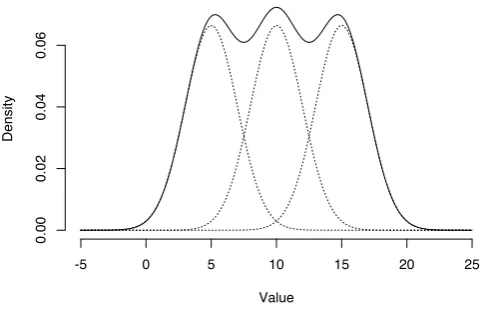
See figure 2.5 for an example of a (Gaussian) mixture distribution. A probability density function such as (2.4) can be used to approximate, arbitrarily close, any finite, continuous density function. This makes it suitable to be applied to a wide range of problems. The simplest example of a distribution like this, is a single component Gaussian distribution.

(26)

[image:26.595.185.433.106.262.2]

Figure 2.5: Density of a mixture of three normal distributions (µ = {5,10,15}, σ = 2) with equal weights. Each component is shown as a weighted density (each integrating to 1/3) [30]

described in the remainder of this chapter. For the proof, see Appendix A. The main reason that we mention mixture distributions, is that most of the literature on HMMs seems to omit this equivalence result. We will not use mixture distributions in this research.

2.4 Estimating the model parameters

Up to this point, we have described the most important elements that make up a general HMM. Before we can use the HMM in real world applications, three key problems have to be solved. These problems are the following.

Problem 1: Given an observation vector O = O1O2· · ·OT and a model λ = (A,B, πππ), how to efficiently compute the probability P(O|λ) that this observation vector was generated by the model?

This is the evaluation problem. It can also be viewed as the problem of scoring how well a given model matches a given observation. The solution allows you to choose the best match among competing models.

(27)

Problem 3: How to adjust the model parameters λ = (A,B, πππ) to maximize P(O|λ) for given data O?

[image:27.595.101.476.254.455.2]

This is the learning problem. It can be viewed as training a model to best fit the observed data. The observation sequence used to adjust (“train”) the model parameters is called a training sequence.

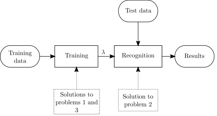
Figure 2.6 gives a schematic overview of why it is necessary to solve these prob-lems and how the solutions to these three probprob-lems are applied to the classification process.

Training data

Test data

Results λ

Solution to problem 2

Training Recognition

Solutions to problems 1 and

3

Figure 2.6: The training process alternates between applying the solutions to prob-lem 1 and 3; to score how well a model fits the training data, and to update the parameters until some level of optimality is reached. The fully trained model then uses the solution to problem 2 to classify independent test data.

2.4.1 Solution to problem 1

Letλ= (A,B, πππ) be a given model, letO=O1O2· · ·OT be an observation sequence, and letX =X1X2· · ·XT be a state sequence. By the definition of the distributions A,B andπππ, we have

(28)

We are interested in finding P(O|λ). A direct approach to compute this quantity would be to sum over all possible state sequencesX:

P(O|λ) =X

X

P(O,X |λ)

=X

X

P(O|X, λ)P(X |λ)

=X

X

πX1bX1(O1)aX1,X2bX2(O2)· · ·aXT−1,XTbXT(OT).

Here the first step makes use of conditional probability. However, since there areNT possible state sequences, this approach would require (2T−1)NT multiplications and NT−1 additions and is therefore computationally infeasible. Clearly a more efficient procedure is required. Such a procedure exists and is called the Forward-Backward algorithm [24].

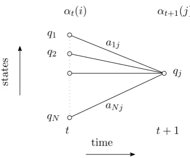
The Forward-Backward algorithm

LetO1:t_{= (O}

1, . . . , Ot) be the observation sequence until timet. For 1≤t≤T and 1≤j≤N, define the forward variable in the following way:

αt(j) :=P O1:t, Xt=qj|λ

. (2.5)

Now, omitting theλ’s for the sake of brevity, and using conditional probability: αt(j) =P O1:t−1, Ot, Xt=qj

= N

X

i=1

P O1:t−1, Xt−1=qi, Xt=qj, Ot

= N

X

i=1

P Xt=qj, Ot|O1:t−1, Xt−1 =qi

·P O1:t−1, Xt−1 =qi

= N

X

i=1

P Xt=qj, Ot|O1:t−1, Xt−1 =qi

αt−1(i)

= N

X

i=1

P(Xt=qj, Ot|Xt−1=qi)αt−1(i)

= N

X

i=1

aijbj(Ot)αt−1(i)

=

" _N X

i=1

αt−1(i)aij

#

bj(Ot)

(29)

states

time q1

q2

qN

qj

t t+ 1

αt(i) αt+1(j) a1j

[image:29.595.184.371.94.249.2]

aN j

Figure 2.7: To calculate the value of the forward variable at time t+ 1, you only need the values of the forward variables for all states at timet.

1. Initial step:

α1(j) =πjbj(O1), 1≤j ≤N

2. For 1≤t≤T−1, and 1≤j≤N

αt+1(j) =

" _N X

i=1

αt(i)aij

#

bj(Ot+1)

3. Termination. From the definition ofαj(t), we find

P(O|λ) = N

X

j=1 αT(j)

To calculate P(O|λ) we need N(N + 1)(T −1) +N ≈ N2_T _{multiplications and} N(N −1)(T −1) +N additions. In other words, using the forward algorithm has an enormous computational advantage over the direct approach as described above.

Let Ot+1:T _{= (O}

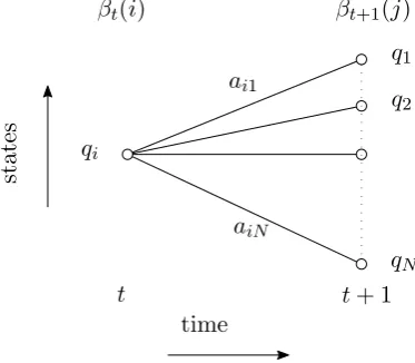
t+1, . . . , OT) be the observation sequence from time t+ 1 until timeT. Then in similar fashion, we can also define a backward variable:

βt(i) :=P Ot+1:T|Xt=qi, λ

(30)

Again omitting theλ’s and using conditional probability:

βt(i) = N

X

j=1

P Ot+1:T_|_X

t=qi, Xt+1 =qj

P(Xt+1 =qj|Xt=qi)

= N

X

j=1

P Ot+1:T|Xt+1=qj

aij = N X j=1

P(Ot+1|Xt+1=qj)·P Ot+2:T|Ot+1, Xt+1=qj

aij = N X j=1

bj(Ot+1)P Ot+2:T|Xt+1 =qj

aij = N X j=1

aijbj(Ot+1)βt+1(j)

See figure 2.8 for an illustration of the calculation of the backward variables.

states time q1 q2 qN qi

t t+ 1

ai1

aiN

[image:30.595.207.394.357.520.2]

βt(i) βt+1(j)

Figure 2.8: To calculate the value of the backward variable at timet, you only need the values of the forward variables for all states at timet+ 1.

So the βt(i) can then also be computed recursively: 1. Initial step:

βT(i) = 1, 1≤i≤N 2. Fort=T−1, T −2, . . . ,1, and 1≤j ≤N

βt(i) = N

X

j=1

(31)

3. Termination.

P(O|λ) = N

X

i=1

P(O|X1 =qi, λ)πi

= N

X

i=1

P(O1|X1 =qi, λ)P O2:T|O1, X1=qi, λ

πi = N X i=1

bi(O1)P O2:T|X1 =qi, λ

πi = N X i=1

bi(O1)β1(i)πi

The computational cost of using the backward algorithm is comparable to that of the forward algorithm.

It is possible to combine both these approaches: P(O, Xk =qj|λ) =P

O1:k_{, X}

k=qj|λ

POk+1:T_|O1:k_{, X}

k=qj, λ

=P

O1:k, Xk=qj|λ

P

Ok+1:T|Xk=qj, λ

=αk(j)βk(j) and hence

P(O|λ) = N

X

j=1

αk(j)βk(j). (2.7)

For the solution to problem 2, [28, p. 261–263] proved very helpful. Let O = O1O2· · ·OT be an observation sequence. Given this data we want to find the state sequence that best explains the observation. What exactly this best explanation is, depends on what we are trying to accomplish.

Individually most likely states

If the objective is to maximize the number of individually most likely states, we need to compute

arg max

j P(Xt=qj|O, λ), 1≤j≤N,

(32)

and 1≤j≤N, define

γt(j) : =P(Xt=qj|O, λ) (2.8) = P(Xt=qj,O|λ)

P(O|λ) = Pαt(j)βt(j)

iαt(i)βt(i) .

So, the optimal predictors at timet of the index of the statei∗_t and the most likely stateX_t∗ itself are then given by

i∗_t = arg max j γt(j) = arg max

j

αt(j)βt(j)

P

iαt(i)βt(i)

(2.9)

X_t∗ =qi∗t (2.10)

A downside of considering only the individually most likely states, is that the obtained optimal state sequence might allow for impossible state transitions ifaij = 0 for some individually optimal i, j. It simply provides us with the most likely state at each clock time without regard to network structure, neighboring states or the length of the observation sequence.

Viterbi algorithm

Alternatively, we can regard the sequence of states as a single entity. The objective is now, given some observation sequence, to choose the sequence of states (path) whose conditional probability as a whole is maximal. The algorithm that solves this problem is called the Viterbi algorithm. Let X1:t_{= (X}

1, . . . , Xt) be the vector representation of the first t states, and let O1:t _{= (O1, . . . , O}

t) be the observation sequence until time t. The problem of interest is to find the sequence of states X1, . . . , Xt that maximizesP X1:t|O1:t, λ

. Since

P X1:t|O1:t, λ= P X

1:t_,_O1:t_|_λ

P(O1:t_|_λ) and P O1:t_|_λ

only depends on the model parameters (see previous section), this maximization problem is equivalent to finding the sequence of statesX1, . . . , Xtthat maximizes P X1:t_,_O1:t_|_λ

. For the sake of brevity, we will omit the λ term when denoting these probabilities.

(33)

with the partial best path ending at stateqj at time t. Formally: δt(j) := max

X1:t−1

P X1:t−1, Xt=qj,O1:t

(2.11) For t = 1, the most probable path to a state does not sensibly exist; there are no preceding states. However, we can use the probability of being in that state given t= 1 and the observed signal O1:

δ1(j) =P(X1 =j, O1) =πjbj(O1)

Recall that the Markov property says that the probability of transitioning to the next state, given a sequence of the previous states, depends only on the current state. The probability of the most probable path to stateXtcan now be recursively calculated in the following way:

δt(j) = max

X1:t−1

P X1:t−1, Xt=qj,O1:t

= max i

max

X1:t−2P X

1:t−2_{, X}

t−1=qi, Xt=qj,O1:t−1, Ot

= max i max

X1:t−2P X

1:t−2_{, X}

t−1=qi,O1:t−1

·P Xt=qj, Ot|X1:t−2, Xt−1 =qi,O1:t−1

= max i max

X1:t−2P X

1:t−2_{, X}

t−1=qi,O1:t−1

·P(Xt=qj, Ot|Xt−1=qi)

= max i

P(Xt=qj, Ot|Xt−1=qi)· max

X1:t−2P X

1:t−2_{, X}

t−1 =qi,O1:t−1

= max

i [aijδt−1(i)]bj(Ot)

So, to calculateδt(·), we only needδt−1(i) for all states 1≤i≤N. Having calculated these probabilities, it is possible to record which preceding state was the one to generate δt(i), i.e. in which state the process must have been at time t−1 if it is to arrive optimally at stateqi at time t. To keep track of the states that maximize theδ’s, define

Ψt(j) = arg max

i [δt−1(i)aij]. (2.12) The Ψ’s answer the question “if I am here, by what path is it most likely I arrived?”. Summarizing, the complete Viterbi algorithm now looks like this:

1. Initialization:

(34)

2. Recursion:

δt(j) = max

1≤i≤N[δt−1(i)aij]bj(Ot), 2≤t≤T, 1≤j≤N Ψt(j) = arg max

1≤i≤N[δt−1(i)aij], 2≤t≤T, 1≤j≤N

3. Termination:

P∗ = max

1≤i≤N[δT(i)] i∗_T = arg max

1≤i≤N[δT(i)] X_T∗ =qi∗

T

4. Path backtracking:

i∗_t = Ψt+1(i∗t+1), t=T−1, T−2, . . . ,1 X_t∗ =qi∗t

Here P∗ is the total probability of the most likely path given some observation sequence O, i∗_t is the index of the most likely state at time t, and X_t∗ is the most likely state at timet of the most likely path.

The third problem is to adjust the parameters (A,B, πππ) of a HMM λto best fit an observation sequence O. Formally:

λ∗ = arg max

λ P(O|λ)

There is no known way to analytically solve for such a λ. In fact, given any finite observation sequence, there is no optimal way of estimating the model parameters [24]. However, it is possible to use an iterative procedure called the Baum-Welch re-estimation algorithm to find a local maximum forP(O|λ).

Given some model λ and an observation sequence O, define ξt(i, j) to be the probability of being in stateqi at time t, and state qj at timet+ 1:

(35)

backward variables:

ξt(i, j) =

P(Xt=qi, Xt+1=qj,O|λ) P(O|λ)

= P Xt=qi, Xt+1=qj,O

1:t_,_Ot+1:T_|_λ

P(O|λ) = P Xt+1 =qj,O

t+1:T_|_X

t=qi,O1:t, λ

·P Xt=qi,O1:t|λ

P(O|λ) = P Xt+1 =qj, Ot+1,O

t+2:T_|_X

t=qi,O1:t, λ

·P Xt=qi,Ot|λ

P(O|λ)

= 1

P(O|λ)

P Ot+2:T_|_X

t=qi, Xt+1 =qj,O1:t, Ot+1, λ

·P Xt+1=qj, Ot+1|Xt=qi,O1:t, λ

·P Xt=qi,O1:t|λ

= 1

P(O|λ)

P Ot+2:T|Xt+1=qj, λ

·P(Xt+1=qj, Ot+1|Xt=qi, λ)

·P Xt=qi,O1:t|λ

= αt(i)aijbj(Ot+1)βt+1(j) P(O|λ)

Here the forward variableαt(i) accounts for the firsttobservations, ending at state qi at time t. The term aijbj(Ot+1) accounts for the transition to state qj at time t+1 along with the observation of signalOt+1. Lastly, the backward variableβt+1(j) accounts for the remainder of the observation sequence.

Recall that in equation (2.8) we defined

γt(i) =P(Xt=qi|O, λ).

γt(i) can be related toξt(i, j) by summing overj:

γt(i) = N

X

j=1

ξt(i, j).

Define a counting variable

It:=

(

(36)

Then

E[# visits to stateqi] =E[# transitions from state qi] =E

"_T₋₁ X

t=1 It

#

= T−1

X

t=1

E[It]

= T−1

X

t=1 γt(i)

Similarly,

E[# transitions from state qi to stateqj] = T−1

X

t=1

ξt(i, j)

We now have the building blocks to write down the re-estimation formulas. The formula for the initial distribution is simply the probability of being in state qi at timet= 1:

ˆ

πi =γ1(i), 1≤i≤N. (2.14)

The re-estimation formula for aij is the expected number of transitions from qi to qj divided by the expected total number of transitions out ofqi:

ˆ aij =

PT−1

t=1 ξt(i, j)

PT−1

t=1 γt(i)

, 1≤i, j≤N. (2.15)

The re-estimation formula for a discrete signal distribution bj(k) is the expected number of visits to stateqj wherekis the observed signal, divided by the expected total number of visits to state qj:

ˆ bj(k) =

PT

t=1Itkγt(i)

PT

t=1γt(i)

, 1≤j≤N,1≤j ≤M (2.16)

where

I_tk:=

(

1, Ot=vk 0, otherwise.

(37)

If a HMM consists of just one state, the re-estimation would be easy. The estimators ofµ and Σ would just be the averages:

ˆ µ= 1

T T

X

t=1 Ot,

ˆ Σ = 1

T T

X

t=1

(Ot−µ)(Ot−µ)>.

In practice, there usually are multiple states and because the underlying state se-quence is unknown there is no direct assignment of observation vectors to individual states. The solution is to assign each observation to every state in proportion to the probability of the model being in a certain state at a certain time. Let γt(j) again denote the probability of being in statej at timet, the re-estimation formulas then become the following weighted averages:

ˆ µj =

Pt

t=1γt(j)Ot

Pt

t=1γt(j)

, (2.17)

ˆ Σj =

Pt

t=1γt(j)(Ot−µ)(Ot−µ)

>

Pt

t=1γt(j)

. (2.18)

One can check that all of the above estimators are the Maximum Likelihood Estimators (MLEs), see for example [6]. The complete iterative procedure is now as follows:

1. Initialization of the modelλ= (A,B, πππ).

2. Re-estimation. Compute ˆA, ˆB and ˆπππ and define an adjusted model ˆλ = ( ˆA,B,ˆ πππ).ˆ

(38)

(39)

Chapter 3

Modeling activities through

HMMs

3.1 Introduction

As mentioned earlier, HMMs were first successfully applied in the field of speech recognition. HMMs are a suitable modeling choice because they are able to incor-porate the sequential quality of speech. Typical daily human activities share this sequential quality. For example, in the same way words are divided into phonemes, activities can be separated into a number of distinct parts.

The first section of this chapter is about the experimental data set we perform our experiments on. Here we go into the details of the acquisition of kinematic data, which includes a description of the sensors, the locations where they are placed, how many are needed and the type of data that is recorded. This is followed by a section on the application of HMMs to physical activities and a discussion of the initialization of the HMM parameters and the training and testing processes of the classifier. The final section is about the software implementation of the algorithms described in the previous chapter.

3.2 Experimental data

(40)

3.2.1 Data acquisition and processing

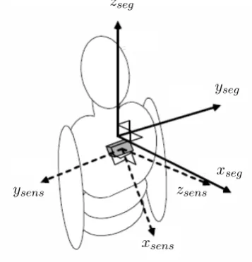
For the recording of data we use MTw motion tracking sensors [17], developed by the Enschede based company Xsens [8]. These sensors record three-dimensional an-gular velocity, acceleration and magnetic field data. A sensor cannot be placed in the exact same spot every time. Because of this, and to make the data comparable to data recorded by other sensors placed on the subject, some segment calibration measurements are performed. These calibration measurement are needed to deter-mine the orientation of each sensor worn by a subject, and are used to rotate the sensor coordinate systems to a universal coordinate system. See figure 3.1 for a schematic representation of this process.

zseg

yseg

xseg ysens

[image:40.595.212.391.264.450.2]

xsens zsens

Figure 3.1: The dashed arrows represent the sensor orientation on the subject, and the solid arrows represent the segment orientation in the universal coordinate system.

The sensors are wireless and weigh approximately 27 grams, so they can be worn easily and unobtrusively by any subject. We want the sensor configuration to be minimal for the subject: as few sensors as possible, positioned as unobtrusively as possible. In the previous RRD study with patients with DMD [44], sensors were placed on the trunk, the head, the lower and upper dominant arm and the dominant hand. For the subject it would be much better if we could lose the sensor positioned on the head.

The recorded data is cleaned up and low pass filtered. The cut off frequency of the low pass filter for the acceleration data is 7 Hz, the cut off frequency for the gyroscopic data is 5 Hz. The filtering is performed to obtain a more smooth signal in order to apply down sampling. The resulting signal has a frequency of 25 Hz. The reason to perform down sampling is human movement cannot exceed a frequency of

(41)

3.3 Application of HMMs

It is possible to observe human activities as a sequence of smaller, basic movements. For a specific activity, the order of these basic movements is always the same. For example, the activity ’picking up an object’ can be split into a sequence of five separate actions, namely (1) a downward acceleration; (2) a downward deceleration; (3) no movement; (4) an upward acceleration; and finally (5) an upward deceleration. To understand a typical human activity in terms of a HMM, we will start with the hidden Markov chain and what it should represent. As a starting point, and to impose a temporal order to the model, we choose for a left-to-right architecture, with delta equal to 1 (see also 2.3.2). We let each state in this representation correspond to one of the basic movements of an activity. For the activity ’picking up an object’ as described above, the number of states then will be five. Because of the chosen architecture each of these states must be visited, which also means that it is not possible to skip any of the basic movements of the activity. With this we have enough information to implicitly define the transition probability matrixA. It should be an upper triangular matrix with all elements equal to zero, except those on and directly above the diagonal.

The second model parameter, namely the initial state distribution, is easy for the chosen Markov chain architecture. Since we are only considering left-to-right models, all chains must start from the left-most state. This means that the initial distribution will be of the formπππ={1,0, . . . ,0}.

The third model parameter is the signal probability distribution in each state. We have assumed that a state corresponds to a small, basic movement, which is characterized by the data being stationary in some sense (e.g. downward acceleration or no movement at all). In the theoretical ideal case, where specific human activities are always performed in the exact same way, and any resulting recorded data is very ’clean’, it would be possible to observe these stationary parts across all parallel data channels. The resulting sequence of these stationary parts then makes up a complete activity.

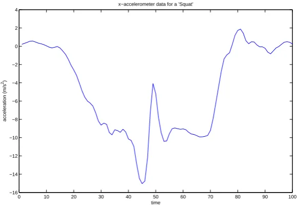
To some extent it is indeed possible to observe these stationary parts in real life measurements. See for example figure 3.2. To account for noise in the signal and variation between different examples of the same activity, we model each state by a normal distribution with meanµand covariance matrix Σ. Data points can then be probabilistically matched to whatever state was most likely to have generated them. We now have covered all parameters λ= (A,B, πππ) that make up a HMM. For each activity that needs to be classified, a separate HMM needs to be defined. The total of these activities make up our dictionary.

3.3.1 Initialization

(42)

0 10 20 30 40 50 60 70 80 90 100 −16

−14 −12 −10 −8 −6 −4 −2 0 2 4

x−accelerometer data for a ’Squat’

time

acceleration (m/s

[image:42.595.163.454.108.313.2]

2)

Figure 3.2: An example of an accelerometer data channel of a subject performing a ’squat’. The sensor was positioned on the spine. It is possible to observe stationary parts within the time series.

is important is that all illegal state transitions have probability zero. The nonzero elements can be given any positive value between zero and one, the only constraint is that each row of the matrix should sum up to one.

For the initialization of the signal probability distribution the values of µ and Σ need to be specified. In contrast to the matrix A, here the initial values play a more important role because they determine the initial location of the hidden Markov chain states within the state space. Since the Baum-Welch algorithm is a local optimizer, and since it is as of yet unknown to us how ’mountainous’ the space is where Baum-Welch operates, a smart choice of the initial values ofµand Σ seems essential.

However, for our preliminary testing, we will provide all HMMs with a ’flat’ start. Allµj and Σj will be given the value of the mean and variance of the complete training dataset. We will return to this question in chapter 5 and address it in more detail.

3.3.2 Training and testing

To train the HMMs, we need to provide a set of training data. This training set consists of a sequence of manually labeled examples of each of the activities from the dictionary. The activities are recorded in a random order, to make sure the classifier is not trained to recognize them in a certain order.

(43)

through application of the iterative Baum-Welch algorithm (see section 2.4.3). An open question is how often to iterate it. If a HMM goes through too many iterations, it may adjust to very specific random features of the training data, that have little or nothing to do with the target activity. When the model overfits the data, the performance on the training examples may still increases while at the same time the performance on unseen data becomes worse. For the case of speech recognition, the HTK manual [43] suggests that five iterations should be sufficient. Compared to speech, our data is of a higher dimension, so maybe a few more iterations will be needed.

The trained models can now be provided with an independent test data set. The test data set again consists of a sequence of randomly ordered activities. The Viterbi algorithm (see section 2.4.2) is applied to transcribe the data.

3.4 Software implementation

All the above algorithms and functionalities are implemented using the Hidden Markov Toolkit software package (HTK 3.4), which was developed at the Machine Intelligence Laboratory of the Cambridge University Engineering Department [1]. The toolkit is designed to run with a traditional command-line style interface. At RRD a shell was built around the HTK tools in a Labview environment. This was done to increase the user-friendliness of the software and make it possible to run large automated batches of train-and-test sessions with varying parameters.

An important aspect of the implementation that needs to be addressed here is the handling of probabilities. Both the Baum-Welch algorithm (through the Forward-Backward calculations) and the Viterbi algorithm need to calculate long products of probabilities. These products tend to zero exponentially fast, so there is the risk of numerical underflow. To avoid this problem, we use the logarithm of the probabilities instead. This means that all products of probabilities are transformed into sums.

3.4.1 HERest training tool

The training procedure is carried out by the HTK tool called HERest, which applies the Baum-Welch algorithm. HERest requires a transcripted sequence of continuous activities as its input. It concatenates all the HMMs corresponding to the training sequence to construct a single composite HMM. The training examples of the various activities are processed to re-estimate all parameters of each individual HMM within the composite HMM. In this process, the transcriptions are only used to identify the sequence of activities; it is not necessary to include the start and end times of individual activities.

(44)

is determined by the number of input data channels, and hence we consider the values of the global mean and variance per data channel. The flat start procedure implies that during the first re-estimation cycle, each training example of an activity will be uniformly segmented. The hope then is that enough hidden Markov states align with their actual realizations (i.e. the smaller basic movements that make up activities), so that after the subsequent training iterations the HMMs align to the training data as intended. Prior studies suggest that this is indeed what happens.

3.4.2 HVite recognition tool

The classification process is handled by the HTK tool HVite. The recognition of a single activity can be achieved through straightforward application of the Viterbi al-gorithm as described in the chapter on HMMs. In theory this would work as follows. Recall again that for each activity a separate HMM is defined. For each of these HMMs the total probability that some observed data sequence was generated by one of these HMMs can be calculated through application of the Viterbi algorithm. The most likely HMM then must have been the one to have generated the observation and the classification is complete.

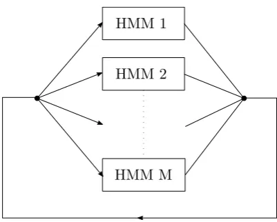
In practice however, test data will consist of a sequence of unknown activities, the start and end times of which are also unknown. HVite extends the Viterbi algorithm in the following way to handle sequential activity recognition [42]. All separate activity HMMs are connected in a looped composite model (see figure 3.3). It is again possible to apply the Viterbi algorithm to this model to calculate the most likely sequence of states through the composite network. The difference is that it now also operates on a macro (whole activities) level instead of just on a micro (hidden Markov state) level. The output of the HVite function is the most likely sequence of activities, including activity boundary information and the total log probability for each recognized activity.

Another internal HTK parameter that influences the recognition, is the word insertion penalty p. This parameter p influences the number of expected activities within an activity sequence by adding an offset to the log probability of a possible classified activity. A larger value of p means that you expect a smaller number of activities, which will result in less false positives, i.e. recognizing something where there is nothing to recognize. At the same time, a larger penalty also means that the number of false negatives, i.e. missing an activity, will increase. Within the Labview environment, some automated testing is performed to find the optimal value of the word insertion penalty. Optimal here means that the total number of errors is as small as possible.

3.4.3 HResults evaluation tool

(45)

HMM 1

HMM 2

[image:45.595.185.386.96.257.2]

HMM M

Figure 3.3: Given an unknown sequence of activity data, HVite connects all the HMMs in the dictionary in a looped composite model and calculates the path through the network that is most likely to have generated the data.

mistakes. It could recognize the wrong activity, which we will call a substitution errorS. Also, it could miss an activity, which we will call a false negative or deletion error D. Lastly, it could recognize an activity where there is nothing to classify, which we will call a false positive or insertion errorI.

The last error type is usually the worst. If the software classifies some activity, you want to be as certain as possible that there actually was something to classify. If the number of insertion errors becomes too large, it can make you doubt all your results. In case of a substitution error, at least you are certain that there is an actual activity to classify. In case of deletion error, you are missing an activity but the accuracy of the other results does not decrease. This is why we think avoiding insertion errors is the most important.

HResults uses the following output statistics: Correctness = N −D−S

N ·100% Accuracy = N −D−S−I

N ·100%,

WhereN is the total number of activities in the test data set. Note that theoretically the Accuracy could become negative, but in some cases this number might be a more representative measure of the performance of the recognizer than the correctness.

3.4.4 HTK flowchart

(46)

Training data

Test data

HResults

Determine optimalp

[image:46.595.123.496.278.475.2]

HERest HVite

(47)

Chapter 4

Data preprocessing

4.1 Introduction

To make the training process more efficient and to improve the classification results of the HMM-based classifier, we apply preprocessing to optimize the data that go into the model. Optimizing data means maximizing the amount of information and minimizing the amount of redundant data (noise) they contain. A previous study [31] also looked into this problem and considered several preprocessing techniques. The most promising of these techniques is Principal Components Analysis (henceforth PCA).

Other studies also combined HMMs with PCA. See for example [27] on face recognition or [37] on handwriting recognition. More relevant to our problem are for example [3] and [9], who applied PCA on motion data before training the HMMs. In this chapter we will explain the theory of principal components analysis, discuss its limitations and investigate its applicability to our problem.

4.2 Goals of data optimization

First we need to define what maximizing the amount of information and minimizing the amount of redundancy and noise exactly means. When constructing a HMM to optimally describe a certain activity, it is difficult to know beforehand which elements of that activity best capture its essence and need to be represented in the HMM. In this discussion, we will consider processed data that leads to better classification results to be more optimal data.

(48)

An important aspect of data optimization is dimensionality reduction. Not all of the recorded channels will contain the same amount of information. Dimensionality reduction is the process of reducing the number of variables under consideration, while preserving as much essential information as possible.

4.3 Theory of PCA

Principal Components Analysis (henceforth PCA) combines all of the aspects de-scribed in the previous paragraph. The idea of PCA is as follows. Imagine recording in three dimensions the motion of a ball hanging from a spring (example inspired by [29]). Most likely, the largest part of the variation in the recorded data will be in the direction of the spring (the verticalz-axis). Any movement of the ball in the direction of the x and y axes can be regarded as noisy perturbations around the z-axis.

Now imagine a more general experiment where it is not so clear beforehand how to choose the direction of the axes you are recording and how many dimensions you should take into consideration. PCA looks for a translation and rotation of the recorded axes to a new coordinate system where the amount of information in each dimension is optimized. This way, it becomes easier to discover underlying structure in the data. In case of the ball-on-a-string experiment, where you recorded three-dimensional data but did not know the best way to choose the axes along which to record, the underlying structure revealed by PCA will tell you the direction that contains most variation (or information) and hence the most likely direction of the spring.

In a more general sense, PCA transforms the data from the original space to a new space of the same dimension. Through this transformation, PCA may make it easier to see that the data are in fact grouped around a manifold of much lower dimension than the original space where the data were recorded. This could be helpful when you are trying to reduce the dimensionality of the data. Dimensions that contain little variation, and hence also little information, may be discarded before feeding the data set to the classifier.

(49)

4.3.1 Maximum variance formulation

Consider a set ofD-dimensional, observation vectors {xn},n= 1, . . . , N. The aim is to project the data onto a lower dimensional subspace having dimensionM ≤D, while maximizing the variance of the projected data.

For simplicity, let us first consider projecting the data onto a one-dimensional space. We can describe this new space using aD-dimensional vectoru1 with length 1 (i.e. ku1k= 1). Each observation vector xn is projected onto a scalaruT1xn. The mean of the projected data is then given byuT

1x, where

x= 1 N

N

X

n=1

xn, (4.1)

the variance of the projected data is given by 1

N N

X

n=1

{uT₁xn−u1Tx}2=uT1Su1, (4.2)

whereS is the covariance matrix defined by

S= 1 N

N

X

n=1

(xn−x)(xn−x)T. (4.3)

To find the direction for which the projected variance is maximal, we maximize equation (4.2) with respect to the vectoru1. Note that the fact that we have chosen

ku1k= 1 makes this a constrained optimization and we have arrived at the following optimization problem:

(

maxuT₁Su1,

s.t.ku1k= 1. (4.4)

To find u1, introduce a Lagrange multiplier λ1 and solve the unconstrained maxi-mization problem

max u1

uT₁Su1+λ1(1− ku1k). (4.5) Calculating the derivative with respect to u1 and setting the result equal to zero, gives

Su1 =λ1u1. (4.6)

This means that u1 must be an eigenvector of the covariance matrix S. Left-multiplying this equation by uT₁ and using thatku1k= 1,

(50)

we see that the variance of the projected data is equal to the eigenvalue λ1. This means that the variance is maximal for the eigenvectoru1associated with the largest eigenvalue λ1 of the covariance matrix S. We call this eigenvector u1 the first principal component.

Since the covariance matrix is a symmetric matrix, all its eigenvectors are orthog-onal. This means that we can define the additional principal componentsu2, . . . ,uM in an incremental fashion by choosing them to be the eigenvectors associated with the remaining M −1 largest eigenvalues λ2, . . . , λM. The amount of variation ex-plained by componenti is given by

λi

PM

j=1λj

. (4.8)

Using the eigenvectors, we can define a transformation matrixP = [u1· · ·uM]. The original dataX= [x1· · ·xN] can now be expressed in the new principal component space Y through the following transformation:

Y =PTX. (4.9)

4.3.2 Limitations of PCA and application to motion data

PCA can only be meaningfully applied to a data set if a number of assumptions is satisfied [29]. The most important motivation of applying PCA is to decorrelate a data set. For this to work, it must be true that the original data is arranged along orthogonal axes. Further, decorrelation also removes any second or higher order dependencies within the data, so applying PCA to data that do contain higher order dependencies leads to loss of information.

Do these assumptions hold when considering the motion data in our lifting exper-iment? The recorded data consist of accelerometer and gyroscope data. Naturally, anyx-,y- andz-accelerometer and gyroscope data channels are orthogonal. Further, there are no second or higher order dependencies between any of these channels; since we consider freely moving subjects, any value of the acceleration could be combined with any angular velocity.

The third assumption is that we consider a component with low variance to have low information. In other words, if a component has a low variance, we say it must represent noise. This last assumption has an important consequence. Our data consist of different channels. Some of these channels will be of a greater order of magnitude than others. For example, z-accelerometer channels are influenced by gravitation, so on average the measured values will be greater than those of the x- and y-accelerometer channels. Of course this does not necessarily mean that thez-channel contains more information. Simple normalization does not solve this problem, because then the ratio between the channels is not preserved and information might be lost.

(51)

we divide by the standard deviation per signal type. This means that we calculate the standard deviation of all accelerometer channels combined and use it instead for the normalization procedure of a single accelerometer channel. For example, for any x-accelerometer channel, this works as follows:

xacc_norm= x

acc₋_x_¯acc σacc

total

(52)

(53)

Chapter 5

Improving the training process

5.1 Overview of this chapter

In the previous chapters, we have described the full process of describing activities through hidden Markov models. In this chapter we will look at several aspects of the training process that can be improved. Firstly, we will discuss how to choose the number of Markov states that best describes a certain activity. Secondly, we will present a detailed discussion of how HTK applies the Baum-Welch algorithm to train a HMM, and discuss how to improve the results of the training. In the final section we will go into choosing the best possible initial values of those hidden states.

5.2 Optimizing the number of Markov states

When using HTK to train a HMM, the number of hidden states in the model needs to be specified. This number remains fixed throughout the training process. We say that for a certain activity i the number of states N, N > 0, is optimal if it maximizes the accuracy of the recognition results on an independent test data set:

N_optimalacti := max

N {Accuracy(N)} (5.1)

In practice, what will typically happen is that as the number of states increases fromN = 1, the accuracy improves. At some point the number of states is sufficient to capture the essence of the activity you are trying to describe. Additional states will be redundant, since there are no more elements of the activity that are not already described by the existing states. The extra states only give meaning to noise, something which is highly undesirable since it will lead to deterioration of the recognition accuracy.