Proceedings of NAACL-HLT 2018, pages 397–407
Scene Graph Parsing as Dependency Parsing
Yu-Siang WangNational Taiwan University
Chenxi Liu( )
Johns Hopkins University
Xiaohui Zeng
Hong Kong University of Science and Technology
Alan Yuille
Johns Hopkins University
Abstract
In this paper, we study the problem of parsing structured knowledge graphs from textual de-scriptions. In particular, we consider the scene graph representation (Johnson et al., 2015) that considers objects together with their at-tributes and relations: this representation has been proved useful across a variety of vision and language applications. We begin by in-troducing an alternative but equivalent edge-centric view of scene graphs that connect to dependency parses. Together with a careful redesign of label and action space, we com-bine the two-stage pipeline used in prior work (generic dependency parsing followed by sim-ple post-processing) into one, enabling end-to-end training. The scene graphs generated by our learned neural dependency parser achieve an F-score similarity of 49.67% to ground truth graphs on our evaluation set, surpassing best previous approaches by 5%. We further demonstrate the effectiveness of our learned parser on image retrieval applications.1 1 Introduction
Recent years have witnessed the rise of interest in many tasks at the intersection of computer vision and natural language processing, including seman-tic image retrieval (Johnson et al.,2015;Vendrov et al.,2015), image captioning (Mao et al.,2014; Karpathy and Li,2015;Donahue et al.,2015;Liu et al., 2017b), visual question answering (Antol et al.,2015;Zhu et al.,2016;Andreas et al.,2016), and referring expressions (Hu et al., 2016; Mao et al., 2016; Liu et al., 2017a). The pursuit for these tasks is in line with people’s desire for high level understanding of visual content, in particu-lar, using textual descriptions or questions to help understand or express images and scenes.
1Code is available at https://github.com/
Yusics/bist-parser/tree/sgparser
What is shared among all these tasks is the need for acommon representationto establish connec-tion between the two different modalities. The ma-jority of recent works handle the vision side with convolutional neural networks, and the language side with recurrent neural networks (Hochreiter and Schmidhuber,1997;Cho et al.,2014) or word embeddings (Mikolov et al., 2013; Pennington et al.,2014). In either case, neural networks map original sources into a semantically meaningful (Donahue et al.,2014;Mikolov et al.,2013) vector representation that can be aligned through end-to-end training (Frome et al., 2013). This suggests that the vector embedding space is an appropriate choice as the common representation connecting different modalities (see e.g.Kaiser et al.(2017)). While the dense vector representation yields impressive performance, it has an unfortunate lim-itation of being less intuitive and hard to interpret. Scene graphs (Johnson et al.,2015), on the other hand, proposed a type of directed graph to encode information in terms of objects, attributes of ob-jects, and relationships between objects (see Fig-ure1for visualization). This is a more structured and explainable way of expressing the knowledge from either modality, and is able to serve as an al-ternative form of common representation. In fact, the value of scene graph representation has already been proven in a wide range of visual tasks, in-cluding semantic image retrieval (Johnson et al., 2015), caption quality evaluation (Anderson et al., 2016), etc. In this paper, we focus on scene graph generation from textual descriptions.
Previous attempts at this problem (Schuster et al.,2015;Anderson et al.,2016) follow the same spirit. They first use a dependency parser to obtain the dependency relationship for all words in a sen-tence, and then use either a rule-based or a learned classifier as post-processing to generate the scene graph. However, the rule-based classifier cannot
a young boy in front of a soccer goal a soccer ball in the air
a man standing with hands behind back a woman wearing a purple shirt a young boy wearing a black uniform the roof is brown
the ball is white
a soccer ball on the ground a man wearing a red and white shirt people behind the net
goal keeper watching the ball a white ball on the ground goal keeper is wearing gloves a kid is sitting on the ground the man is standing the uniform is black
a red and black backpack sitting on the ground trees outside the fence
blue and white soccer ball
young boy
wear
uniform black
backpack
sit on
ground black
[image:2.595.81.288.62.347.2]red
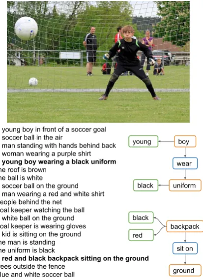
Figure 1: Each image in the Visual Genome (Krishna et al.,2017) dataset contains tens of region descriptions and the region scene graphs associated with them. In this paper, we study how to generate high quality scene graphs (two such examples are shown in the figure) from textual descriptions, without using image infor-mation.
learn from data, and the learned classifier is rather simple with hand-engineered features. In addition, the dependency parser was trained on linguistics data to produce complete dependency trees, some parts of which may be redundant and hence con-fuse the scene graph generation process.
Therefore, our model abandons the two-stage pipeline, and uses a single, customized depen-dency parser instead. The customization is neces-sary for two reasons. First is the difference in la-bel space. Standard dependency parsing has tens of edge labels to represent rich relationships be-tween words in a sentence, but in scene graphs we are only interested in three types, namely objects, attributes, and relations. Second is whether every word needs a head. In some sense, the scene graph represents the “skeleton” of the sentence, which suggests that empty words are unlikely to be in-cluded in the scene graph. We argue that in scene graph generation, it is unnecessary to require a parent word for every single word.
We build our model on top of a neural
depen-dency parser implementation (Kiperwasser and Goldberg, 2016) that is among the state-of-the-art. We show that our carefully customized de-pendency parser is able to generate high quality scene graphs by learning from data. Specifically, we use the Visual Genome dataset (Krishna et al., 2017), which provides rich amounts of region de-scription - region graph pairs. We first align nodes in region graphs with words in the region descrip-tions using simple rules, and then use this align-ment to train our customized dependency parser. We evaluate our parser by computing the F-score between the parsed scene graphs and ground truth scene graphs. We also apply our approach to im-age retrieval to show its effectiveness.
2 Related Works 2.1 Scene Graphs
The scene graph representation was proposed in Johnson et al.(2015) as a way to represent the rich, structured knowledge within an image. The nodes in a scene graph represent either an object, an at-tribute for an object, or a relationship between two objects. The edges depict the connection and as-sociation between two nodes. This representation is later adopted in the Visual Genome dataset ( Kr-ishna et al.,2017), where a large number of scene graphs are annotated through crowd-sourcing.
The scene graph representation has been proved useful in various problems including semantic im-age retrieval (Johnson et al.,2015), visual question answering (Teney et al., 2016), 3D scene synthe-sis (Chang et al.,2014), and visual relationship de-tection (Lu et al.,2016). ExcludingJohnson et al. (2015) which used ground truth, scene graphs are obtained either from images (Dai et al.,2017;Xu et al., 2017; Li et al., 2017) or from textual de-scriptions (Schuster et al., 2015;Anderson et al., 2016). In this paper we focus on the latter.
In particular, parsed scene graphs are used in Schuster et al.(2015) for image retrieval. We show that with our more accurate scene graph parser, performance on this task can be further improved.
2.2 Parsing to Graph Representations
words without introducing extra nonterminals. In fact, all previous work (Schuster et al.,2015; An-derson et al.,2016) on scene graph generation run dependency parsing on the textual description as a first step, followed by either heuristic rules or simple classifiers. Instead of running two separate stages, our work proposed to use a single depen-dency parser that is end-to-end. In other words, our customized dependency parser generates the scene graph in an online fashion as it reads the tex-tual description once from left to right.
In recent years, dependency parsing with neu-ral network features (Chen and Manning, 2014; Dyer et al.,2015;Cross and Huang,2016; Kiper-wasser and Goldberg,2016;Dozat and Manning, 2016;Shi et al.,2017) has shown impressive per-formance. In particular, Kiperwasser and Gold-berg(2016) used bidirectional LSTMs to generate features for individual words, which are then used to predict parsing actions. We base our model on Kiperwasser and Goldberg(2016) for both its sim-plicity and good performance.
Apart from dependency parsing, Abstract Meaning Representation (AMR) parsing ( Flani-gan et al.,2014;Werling et al.,2015;Wang et al., 2015;Konstas et al.,2017) may also benefit scene graph generation. However, as first pointed out inAnderson et al.(2016), the use of dependency trees still appears to be a common theme in the literature, and we leave the exploration of AMR parsing for scene graph generation as future work. More broadly, our task also relates to entity and relation extraction, e.g. Katiyar and Cardie (2017), but there object attributes are not han-dled. Neural module networks (Andreas et al., 2016) also use dependency parses, but they trans-late questions into a series of actions, whereas we parse descriptions into their graph form. Fi-nally,Krishnamurthy and Kollar(2013) connected parsing and grounding by training the parser in a weakly supervised fashion.
3 Task Description
In this section, we begin by reviewing the scene graph representation, and show how its nodes and edges relate to the words and arcs in dependency parsing. We then describe simple yet reliable rules to align nodes in scene graphs with words in textual descriptions, such that customized depen-dency parsing, described in the next section, may be trained and applied.
3.1 Scene Graph Definition
There are three types of nodes in a scene graph: object, attribute, and relation. LetObe the set of
object classes,Abe the set of attribute types, and Rbe the set of relation types. Given a sentence
s, our goal in this paper is to parsesinto a scene
graph:
G(s) =hO(s), A(s), R(s)i (1)
whereO(s) = {o1(s), . . . , om(s)}, oi(s) ∈ Ois
the set of object instances mentioned ins,A(s)⊆
O(s)× Ais the set of attributes associated with object instances, andR(s)⊆O(s)× R ×O(s)is the set of relations between object instances.
G(s) is a graph because we can first create an object node for every element inO(s); then for ev-ery(o, a)pair inA(s), we create an attribute node
and add an unlabeled edgeo→a; finally for every
(o1, r, o2)triplet inR(s), we create a relation node and add two unlabeled edgeso1 → randr →o2. The resulting directed graph exactly encodes in-formation inG(s). We call this thenode-centric
graph representation of a scene graph.
We realize that a scene graph can be equiva-lently represented by no longer distinguishing be-tween the three types of nodes, yet assigning la-bels to the edges instead. Concretely, this means there is now only one type of node, but we assign aATTRlabel for everyo→aedge, aSUBJlabel for everyo1→redge, and aOBJTlabel for every
r →o2edge. We call this theedge-centricgraph representation of a scene graph.
We can now establish a connection between scene graphs and dependency trees. Here we only consider scene graphs that are acyclic2. The
edge-centric view of a scene graph is very similar to a dependency tree: they are both directed acyclic graphs where the edges/arcs have labels. The dif-ference is that in a scene graph, the nodes are the objects/attributes/relations and the edges have la-bel space{ATTR,SUBJ,OBJT}, whereas in a de-pendency tree, the nodes are individual words in a sentence and the edges have a much larger label space.
3.2 Sentence-Graph Alignment
graphs and words in the textual description, scene graph generation and dependency parsing be-comes equivalent: we can construct the gener-ated scene graph from the set of labeled edges re-turned by the dependency parser. Unfortunately, such alignment is not provided between the re-gion graphs and rere-gion descriptions in the Visual Genome (Krishna et al.,2017) dataset. Here we describe how we use simple yet reliable rules to do sentence-graph (word-node) alignment.
There are two strategies that we could use in deciding whether to align a scene graph node
d (whose label space is O ∪ A ∪ R) with a word/phrasewin the sentence:
• Word-by-word match (WBW):d ↔ wonly
whend’s label andwmatch word-for-word.
• Synonym match (SYN)3: d ↔ w when the
wordnet synonyms ofd’s label containw.
Obviously WBW is a more conservative strategy than SYN.
We propose to use two cycles and each cy-cle further consists of three steps, where we try to align objects, attributes, relations in that or-der. The pseudocode for the first cycle is in Al-gorithm 1. The second cycle repeats line 4-15 immediately afterwards, except that in line 6 we also allow SYN. Intuitively, in the first cycle we use a conservative strategy to find “safe” objects, and then scan for their attributes and relations. In the second cycle we relax and allow synonyms in aligning object nodes, also followed by the align-ment of attribute and relation nodes.
The ablation study of the alignment procedure is reported in the experimental section.
4 Customized Dependency Parsing In the previous section, we have established the connection between scene graph generation and dependency parsing, which assigns a parent word for every word in a sentence, as well as a label for this directed arc. We start by describing our base dependency parsing model, which is neural net-work based and performs among the state-of-the-art. We then show why and how we do customiza-tion, such that scene graph generation is achieved with a single, end-to-end model.
3This strategy is also used in (Denkowski and Lavie, 2014) and (Anderson et al.,2016).
Algorithm 1:First cycle of the alignment pro-cedure.
1 Input: Sentences; Scene graphG(s) 2 Initialize aligned nodesN as empty set
3 Initialize aligned wordsW as empty set 4 foroin object nodes ofG(s)\N do
5 forwins\W do
6 ifo↔waccording to WBWthen 7 Add(o, w);N =N ∪ {o};
W =W ∪ {w}
8 forain attribute nodes ofG(s)\N do
9 forwins\W do
10 ifa↔waccording to WBW or SYN anda’s object node is inN then
11 Add(a, w);N =N ∪ {a};
W =W ∪ {w}
12 forrin relation nodes ofG(s)\N do
13 forwins\W do
14 ifr↔waccording to WBW or SYN
andr’s subject and object nodes are
both inN then
15 Add(r, w);N =N ∪ {r};
W =W ∪ {w}
4.1 Neural Dependency Parsing Base Model
We base our model on the transition-based parser ofKiperwasser and Goldberg(2016). Here we de-scribe its key components: the arc-hybrid system that defines the transition actions, the neural archi-tecture for feature extractor and scoring function, and the loss function.
The Arc-Hybrid System In the arc-hybrid sys-tem, a configuration consists of a stackσ, a buffer β, and a set T of dependency arcs. Given a
sen-tence s = w1, . . . , wn, the system is initialized
with an empty stack σ, an empty arc setT, and β = 1, . . . , n,ROOT, whereROOTis a special in-dex. The system terminates whenσis empty andβ
contains onlyROOT. The dependency tree is given by the arc setT upon termination.
The arc-hybrid system allows three transition actions, SHIFT, LEFTl, RIGHTl, described in
Ta-ble 1. The SHIFT transition moves the first el-ement of the buffer to the stack. The LEFT(l)
Stackσt Bufferβt Arc setTt Action Stackσt+1 Bufferβt+1 Arc setTt+1
σ b0|β T SHIFT σ|b0 β T
σ|s1|s0 b0|β T LEFT(l) σ|s1 b0|β T ∪ {(b0, s0, l)}
σ|s1|s0 β T RIGHT(l) σ|s1 β T ∪ {(s1, s0, l)}
σ|s0 β T REDUCE σ β T
Table 1: Transition actions under the arc-hybrid system. The first three actions are from dependency parsing; the last one is introduced for scene graph parsing.
RIGHT(l) transition yields an arc from the second
top element of the stack to the top element of the stack, and then also removes the top element from the stack.
The following paragraphs describe how to se-lect the correct transition action (and label l) in
each step in order to generate a correct dependency tree.
BiLSTM Feature Extractor Let the word em-beddings of a sentence s be w1, . . . ,wn. An
LSTM cell is a parameterized function that takes as inputwt, and updates its hidden states:
LSTM cell: (wt,ht−1)→ht (2)
As a result, an LSTM network, which simply ap-plies the LSTM cell t times, is a parameterized
function mapping a sequence of input vectorsw1:t
to a sequence of output vectorsh1:t. In our
nota-tion, we drop the intermediate vectorsh1:t−1 and let LSTM(w1:t)representht.
A bidirectional LSTM, or BiLSTM for short, consists of two LSTMs: LSTMF which reads the
input sequence in the original order, and LSTMB
which reads it in reverse. Then
BILSTM(w1:n, i) =
LSTMF(w1:i)◦LSTMB(wn:i) (3)
where ◦ denotes concatenation. Intuitively, the forward LSTM encodes information from the left side of thei-th word and the backward LSTM
en-codes information to its right, such that the vector
vi = BILSTM(w1:n, i) has the full sentence as
context.
When predicting the transition action, the fea-ture function φ(c) that summarizes the current configurationc= (σ, β, T)is simply the concate-nated BiLSTM vectors of the top three elements in the stack and the first element in the buffer:
φ(c) =vs2◦vs1 ◦vs0 ◦vb0 (4)
MLP Scoring Function The score of transition actionyunder the current configurationcis deter-mined by a multi-layer perceptron with one hidden layer:
f(c, y) =M LP(φ(c))[y] (5)
where
M LP(x) =W2·tanh(W1·x+b1) +b2 (6)
Hinge Loss Function The training objective is to raise the scores of correct transitions above scores of incorrect ones. Therefore, at each step, we use a hinge loss defined as:
L= max(0,1− max
y+∈Y+f(c, y
+)
+ max
y−∈Y\Y+f(c, y
−)) (7)
whereY is the set of possible transitions and Y+
is the set of correct transitions at the current step. In each training step, the parser scores all possible transitions using Eqn.5, incurs a loss using Eqn.7, selects a following transition, and updates the con-figuration. Losses at individual steps are summed throughout the parsing of a sentence, and then pa-rameters are updated using backpropagation.
In test time, we simply choose the transition ac-tion that yields the highest score at each step.
4.2 Customization
Redesigning Edge Labels We define a total of five edge labels, so as to faithfully bridge the edge-centric view of scene graphs with dependency parsing models:
• CONT: This label is created for nodes whose label is a phrase. For example, the phrase “in front of” is a single relation node in the scene graph. By introducing the CONT label, we expect the parsing result to be either
in−−−→CONT front−−−→CONT of (8)
or
in←−−−CONT front←−−−CONT of (9)
where the direction of the arcs (left or right) is predefined by hand.
The leftmost word under the right arc rule or the rightmost word under the left arc rule is called theheadof the phrase. A single-word node does not need thisCONTlabel, and the head is itself.
• ATTR: The arc label from the head of an ob-ject node to the head of an attribute node.
• SUBJ: The arc label from the head of an ob-ject node (subob-ject) to the head of a relation node.
• OBJT: The arc label from the head of a rela-tion node to the head of an object node (ob-ject).
• BEGN: The arc label from theROOTindex to all heads of object nodes without a parent.
Expanding Transition Actions With the three transition actions SHIFT, LEFT(l), RIGHT(l), we only drop an element (from the top of the stack) af-ter it has already been associated with an arc. This design ensures that an arc is associated with ev-ery word. However, in our setting for scene graph generation, there may be no arc for some of the words, especially empty words.
Our solution is to augment the action set with a REDUCE action, that pops the stack without adding to the arc set (see Table 1). This ac-tion is often used in other transiac-tion-based de-pendency parsing systems (e.g. arc-eager (Nivre, 2004)). More recently,Hershcovich et al.(2017) andBuys and Blunsom(2017) also included this action when parsing sentences to graph structures.
Parser F-score
Stanford (Schuster et al.,2015) 0.3549 SPICE (Anderson et al.,2016) 0.4469 Ours (left arc rule) 0.4967
Ours (right arc rule) 0.4952 Ours (all SYN) 0.4877 Ours (no SYN) 0.4538
[image:6.595.317.515.63.195.2]Oracle 0.6985
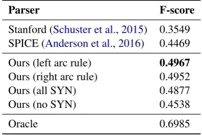
Table 2: The F-scores (i.e. SPICE metric) between scene graphs parsed from region descriptions and ground truth region graphs on the intersection of Vi-sual Genome (Krishna et al.,2017) and MS COCO (Lin et al.,2014) validation set.
We still minimize the loss function defined in Eqn. 7, except that now|Y|increases from 3 to
4. During training, we impose the oracle to select the REDUCEaction when it is inY+. In terms of
loss function, we increment by 1 the loss incurred by the other 3 transition actions if REDUCEincurs zero loss.
5 Experiments
5.1 Implementation Details
We train and evaluate our scene graph parsing model on (a subset of) the Visual Genome ( Kr-ishna et al., 2017) dataset. Each image in Vi-sual Genome contains a number of regions, and each region is annotated with both a region de-scription and a region scene graph. Our training set is the intersection of Visual Genome and MS COCO (Lin et al.,2014) train2014 set, which con-tains a total of 34027 images/ 1070145 regions. We evaluate on the intersection of Visual Genome and MS COCO val2014 set, which contains a total of 17471 images/ 547795 regions.
In our experiments, the number of hidden units in BiLSTM is 256; the number of layers in BiL-STM is 2; the word embedding dimension is 200; the number of hidden units in MLP is 100. We use fixed learning rate 0.001 and Adam optimizer (Kingma and Ba,2014) with epsilon 0.01. Train-ing usually converges within 4 epochs.
We will release our code and trained model upon acceptance.
5.2 Quality of Parsed Scene Graphs
black barrier in front of person Ground truth (node-centric)
black barrier in front SPICE (node-centric): F-score 0.6
of person
node-centric Ours: F-score 1.0
edge-centric
black barrier in front of the person ROOT BEGN
OBJT SUBJ
ATTR CONT CONT
[image:7.595.83.524.64.231.2]black barrier in front of person
Figure 2: Scene graph parsing result of the sentence “black barrier in front of the person”. In the node-centric graphs, orange represents object node, green represents attribute node, blue represents relation node.
Stack Buffer Action
0 black barrier in front of the personROOT SHIFT 1 black barrier in front of the personROOT LEFT(ATTR) 2 barrier in front of the personROOT SHIFT 3 barrier in front of the personROOT SHIFT 4 barrier in front of the personROOT LEFT(CONT) 5 barrier front of the personROOT SHIFT 6 barrier front of the personROOT LEFT(CONT) 7 barrier of the personROOT SHIFT 8 barrier of the personROOT SHIFT 9 barrier of the personROOT REDUCE
10 barrier of personROOT SHIFT
11 barrier of person ROOT RIGHT(OBJT)
12 barrier of ROOT RIGHT(SUBJ)
13 barrier ROOT LEFT(BEGN)
[image:7.595.116.485.284.513.2]14 ROOT
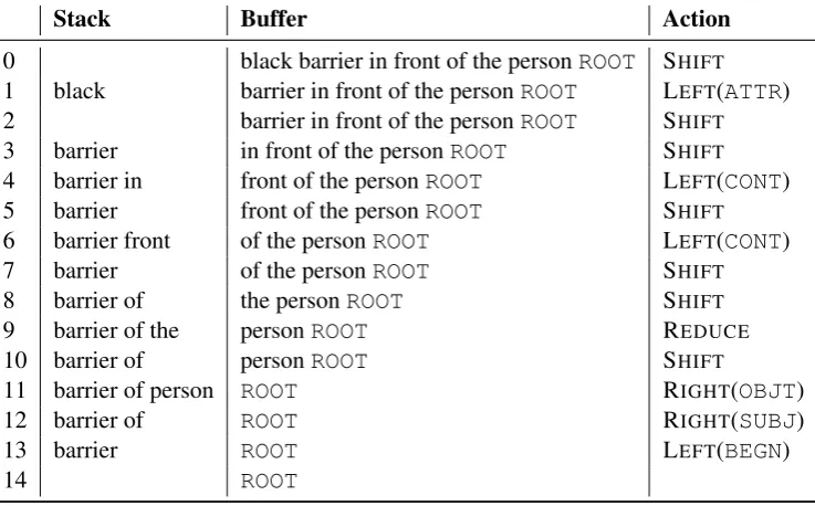
Figure 3: Intermediate actions taken by the trained dependency parser when parsing the sentence “black barrier in front of the person”.
scene graph parsing. Specifically, for every region, we parse its description using a parser (e.g. the one used in SPICE or our customized dependency parser), and then calculate the F-score between the parsed graph and the ground truth region graph (see Section 3.2 ofAnderson et al.(2016) for more details). Note that when SPICE calculates the F-score, a node in one graph could be matched to several nodes in the other, which is problematic. We fix this and enforce one-to-one matching when calculating the F-score. Finally, we report the av-erage F-score across all regions.
Table2summarizes our results. We see that our customized dependency parsing model achieves
an average F-score of 49.67%, which significantly outperforms the parser used in SPICE by 5 per-cent. This result shows that our customized de-pendency parser is very effective at learning from data, and generates more accurate scene graphs than the best previous approach.
Development set Test set
R@5 R@10 Med. rank R@5 R@10 Med. rank
(Schuster et al.,2015) 33.82% 45.58% 6 34.96% 45.68% 5
[image:8.595.88.511.63.134.2]Ours 36.69% 49.41% 4 36.70% 49.37% 5
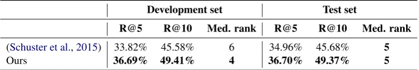
Table 3: Image retrieval results. We follow the same experiment setup asSchuster et al.(2015), except using a different scoring function when ranking images. Our parser consistently outperforms the Stanford Scene Graph Parser across evaluation metrics.
F-score drops in both cases, hence supporting the procedure that we chose.
Second, we study whether changing the direc-tion of CONT arcs from pointing left to point-ing right will make much difference. Table 2 shows that the two choices give very similar per-formance, suggesting that our dependency parser is robust to this design choice.
Finally, we report the oracle score, which is the similarity between the aligned graphs that we use during training and the ground truth graphs. The F-score is relatively high at 69.85%. This shows that improving the parser (about 20% mar-gin) and improving the sentence-graph alignment (about 30% margin) are both promising directions for future research.
Qualitative Examples We provide one parsing example in Figure2 and Figure3. This is a sen-tence that is relatively simple, and the underly-ing scene graph includes two object nodes, one attribute node, and one compound word relation node. In parsing this sentence, all four actions listed in Table 1 are used (see Figure 3) to pro-duce the edge-centric scene graph (bottom left of Figure 2), which is then trivially converted to the node-centric scene graph (bottom right of Fig-ure2).
5.3 Application in Image Retrieval
We test if the advantage of our parser can be propagated to computer vision tasks, such as im-age retrieval. We directly compare our parser with the Stanford Scene Graph Parser (Schuster et al.,2015) on the development set and test set of the image retrieval dataset used inSchuster et al. (2015) (not Visual Genome).
For every region in an image, there is a human-annotated region description and region scene graph. The queries are the region descriptions. If the region graph corresponding to the query is a subgraph of the complete graph of another image,
then that image is added to the ground truth set for this query. All these are strictly following Schus-ter et al. (2015). However, since we did not ob-tain nor reproduce the CRF model used in John-son et al. (2015) and Schuster et al. (2015), we used F-score similarity instead of the likelihood of the maximum a posteriori CRF solution when ranking the images based on the region descrip-tions. Therefore the numbers we report in Table3 are not directly comparable with those reported in Schuster et al.(2015).
Our parser delivers better retrieval performance across all three evaluation metrics: recall@5, re-call@10, and median rank. We also notice that the numbers in our retrieval setting are higher than those (even with oracle) in Schuster et al. (2015)’s retrieval setting. This strongly suggests that generating accurate scene graphs from ages is a very promising research direction in im-age retrieval, and grounding parsed scene graphs to bounding box proposals without considering vi-sual attributes/relationships (Johnson et al.,2015) is suboptimal.
6 Conclusion
The quality of our trained parser is validated in terms of both SPICE similarity to the ground truth graphs and recall rate/median rank when perform-ing image retrieval.
We hope our paper can lead to more thoughts on the creative uses and extensions of existing NLP tools to tasks and datasets in other domains. In the future, we plan to tackle more computer vision tasks with this improved scene graph parsing tech-nique in hand, such as image region grounding. We also plan to investigate parsing scene graph with cyclic structures, as well as whether/how the image information can help boost parsing quality.
Acknowledgments
The majority of this work was done when YSW and XZ were visiting Johns Hopkins University. We thank Peter Anderson, Sebastian Schuster, Ranjay Krishna, Tsung-Yi Lin for comments and help regarding the experiments. We also thank Tianze Shi, Dingquan Wang, Chu-Cheng Lin for discussion and feedback on the draft. This work was sponsored by the National Science Founda-tion Center for Brains, Minds, and Machines NSF CCF-1231216. CL also acknowledges an award from Snap Inc.
References
Peter Anderson, Basura Fernando, Mark Johnson, and Stephen Gould. 2016. SPICE: semantic proposi-tional image caption evaluation. InECCV. Springer, volume 9909 ofLecture Notes in Computer Science, pages 382–398.
Jacob Andreas, Marcus Rohrbach, Trevor Darrell, and Dan Klein. 2016. Neural module networks. In
CVPR. IEEE Computer Society, pages 39–48.
Stanislaw Antol, Aishwarya Agrawal, Jiasen Lu, Mar-garet Mitchell, Dhruv Batra, C. Lawrence Zitnick, and Devi Parikh. 2015. VQA: visual question an-swering. InICCV. IEEE Computer Society, pages 2425–2433.
Jan Buys and Phil Blunsom. 2017. Robust incremental neural semantic graph parsing. InACL. Association for Computational Linguistics, pages 1215–1226.
Angel X. Chang, Manolis Savva, and Christopher D. Manning. 2014. Learning spatial knowledge for text to 3d scene generation. In EMNLP. ACL, pages 2028–2038.
Danqi Chen and Christopher D. Manning. 2014. A fast and accurate dependency parser using neural net-works. InEMNLP. ACL, pages 740–750.
Kyunghyun Cho, Bart van Merrienboer, C¸aglar G¨ulc¸ehre, Dzmitry Bahdanau, Fethi Bougares, Hol-ger Schwenk, and Yoshua Bengio. 2014. Learning phrase representations using RNN encoder-decoder for statistical machine translation. InEMNLP. ACL, pages 1724–1734.
James Cross and Liang Huang. 2016. Incremental parsing with minimal features using bi-directional LSTM. InACL (2). The Association for Computer Linguistics.
Bo Dai, Yuqi Zhang, and Dahua Lin. 2017. Detecting visual relationships with deep relational networks. In CVPR. IEEE Computer Society, pages 3298– 3308.
Michael J. Denkowski and Alon Lavie. 2014. Meteor universal: Language specific translation evaluation for any target language. InWMT@ACL. The Asso-ciation for Computer Linguistics, pages 376–380.
Jeff Donahue, Lisa Anne Hendricks, Sergio Guadar-rama, Marcus Rohrbach, Subhashini Venugopalan, Trevor Darrell, and Kate Saenko. 2015. Long-term recurrent convolutional networks for visual recog-nition and description. In CVPR. IEEE Computer Society, pages 2625–2634.
Jeff Donahue, Yangqing Jia, Oriol Vinyals, Judy Hoff-man, Ning Zhang, Eric Tzeng, and Trevor Dar-rell. 2014. Decaf: A deep convolutional activation feature for generic visual recognition. In ICML. JMLR.org, volume 32 ofJMLR Workshop and Con-ference Proceedings, pages 647–655.
Timothy Dozat and Christopher D. Manning. 2016. Deep biaffine attention for neural dependency pars-ing.CoRRabs/1611.01734.
Chris Dyer, Miguel Ballesteros, Wang Ling, Austin Matthews, and Noah A. Smith. 2015. Transition-based dependency parsing with stack long short-term memory. In ACL (1). The Association for Computer Linguistics, pages 334–343.
Jeffrey Flanigan, Sam Thomson, Jaime G. Carbonell, Chris Dyer, and Noah A. Smith. 2014. A discrimi-native graph-based parser for the abstract meaning representation. In ACL (1). The Association for Computer Linguistics, pages 1426–1436.
Andrea Frome, Gregory S. Corrado, Jonathon Shlens, Samy Bengio, Jeffrey Dean, Marc’Aurelio Ranzato, and Tomas Mikolov. 2013. Devise: A deep visual-semantic embedding model. InNIPS. pages 2121– 2129.
Daniel Hershcovich, Omri Abend, and Ari Rappoport. 2017. A transition-based directed acyclic graph parser for UCCA. In ACL. Association for Com-putational Linguistics, pages 1127–1138.
Sepp Hochreiter and J¨urgen Schmidhuber. 1997. Long short-term memory. Neural Computation
Ronghang Hu, Huazhe Xu, Marcus Rohrbach, Jiashi Feng, Kate Saenko, and Trevor Darrell. 2016. Natu-ral language object retrieval. InCVPR. IEEE Com-puter Society, pages 4555–4564.
Justin Johnson, Ranjay Krishna, Michael Stark, Li-Jia Li, David A. Shamma, Michael S. Bernstein, and Fei-Fei Li. 2015. Image retrieval using scene graphs. In CVPR. IEEE Computer Society, pages 3668–3678.
Lukasz Kaiser, Aidan N. Gomez, Noam Shazeer, Ashish Vaswani, Niki Parmar, Llion Jones, and Jakob Uszkoreit. 2017. One model to learn them all.CoRRabs/1706.05137.
Andrej Karpathy and Fei-Fei Li. 2015. Deep visual-semantic alignments for generating image descrip-tions. In CVPR. IEEE Computer Society, pages 3128–3137.
Arzoo Katiyar and Claire Cardie. 2017. Going out on a limb: Joint extraction of entity mentions and re-lations without dependency trees. InACL. Associa-tion for ComputaAssocia-tional Linguistics, pages 917–928.
Diederik P. Kingma and Jimmy Ba. 2014. Adam: A method for stochastic optimization. CoRR
abs/1412.6980.
Eliyahu Kiperwasser and Yoav Goldberg. 2016. Sim-ple and accurate dependency parsing using bidirec-tional LSTM feature representations. TACL4:313– 327.
Ioannis Konstas, Srinivasan Iyer, Mark Yatskar, Yejin Choi, and Luke Zettlemoyer. 2017. Neural AMR: sequence-to-sequence models for parsing and gen-eration. InACL (1). Association for Computational Linguistics, pages 146–157.
Ranjay Krishna, Yuke Zhu, Oliver Groth, Justin John-son, Kenji Hata, Joshua Kravitz, Stephanie Chen, Yannis Kalantidis, Li-Jia Li, David A. Shamma, Michael S. Bernstein, and Li Fei-Fei. 2017. Vi-sual genome: Connecting language and vision us-ing crowdsourced dense image annotations. Inter-national Journal of Computer Vision123(1):32–73.
Jayant Krishnamurthy and Thomas Kollar. 2013. Jointly learning to parse and perceive: Connect-ing natural language to the physical world. TACL
1:193–206.
Sandra K¨ubler, Ryan T. McDonald, and Joakim Nivre. 2009. Dependency Parsing. Synthesis Lectures on Human Language Technologies. Morgan & Clay-pool Publishers.
Yikang Li, Wanli Ouyang, Bolei Zhou, Kun Wang, and Xiaogang Wang. 2017. Scene graph generation from objects, phrases and caption regions. CoRR
abs/1707.09700.
Tsung-Yi Lin, Michael Maire, Serge J. Belongie, James Hays, Pietro Perona, Deva Ramanan, Piotr Doll´ar, and C. Lawrence Zitnick. 2014. Microsoft COCO: common objects in context. InECCV. Springer, vol-ume 8693 of Lecture Notes in Computer Science, pages 740–755.
Chenxi Liu, Zhe Lin, Xiaohui Shen, Jimei Yang, Xin Lu, and Alan L. Yuille. 2017a. Recurrent multi-modal interaction for referring image segmentation. In ICCV. IEEE Computer Society, pages 1280– 1289.
Chenxi Liu, Junhua Mao, Fei Sha, and Alan L. Yuille. 2017b. Attention correctness in neural image cap-tioning. InAAAI. AAAI Press, pages 4176–4182.
Cewu Lu, Ranjay Krishna, Michael S. Bernstein, and Fei-Fei Li. 2016. Visual relationship detection with language priors. InECCV. Springer, volume 9905 of Lecture Notes in Computer Science, pages 852– 869.
Junhua Mao, Jonathan Huang, Alexander Toshev, Oana Camburu, Alan L. Yuille, and Kevin Murphy. 2016. Generation and comprehension of unambiguous ob-ject descriptions. InCVPR. IEEE Computer Society, pages 11–20.
Junhua Mao, Wei Xu, Yi Yang, Jiang Wang, and Alan L. Yuille. 2014. Deep captioning with mul-timodal recurrent neural networks (m-rnn). CoRR
abs/1412.6632.
Mitchell P. Marcus, Beatrice Santorini, and Mary Ann Marcinkiewicz. 1993. Building a large annotated corpus of english: The penn treebank. Computa-tional Linguistics19(2):313–330.
Tomas Mikolov, Kai Chen, Greg Corrado, and Jeffrey Dean. 2013. Efficient estimation of word represen-tations in vector space.CoRRabs/1301.3781. Joakim Nivre. 2004. Incrementality in deterministic
dependency parsing. InProceedings of the Work-shop on Incremental Parsing: Bringing Engineering and Cognition Together. Association for Computa-tional Linguistics, pages 50–57.
Jeffrey Pennington, Richard Socher, and Christo-pher D. Manning. 2014. Glove: Global vectors for word representation. InEMNLP. ACL, pages 1532– 1543.
Sebastian Schuster, Ranjay Krishna, Angel Chang, Li Fei-Fei, and Christopher D Manning. 2015. Gen-erating semantically precise scene graphs from tex-tual descriptions for improved image retrieval. In
Proceedings of the fourth workshop on vision and language. volume 2.
Damien Teney, Lingqiao Liu, and Anton van den Hen-gel. 2016. Graph-structured representations for vi-sual question answering. CoRRabs/1609.05600.
Ivan Vendrov, Ryan Kiros, Sanja Fidler, and Raquel Urtasun. 2015. Order-embeddings of images and language.CoRRabs/1511.06361.
Chuan Wang, Nianwen Xue, and Sameer Pradhan. 2015. A transition-based algorithm for AMR pars-ing. InHLT-NAACL. The Association for Computa-tional Linguistics, pages 366–375.
Keenon Werling, Gabor Angeli, and Christopher D. Manning. 2015. Robust subgraph generation im-proves abstract meaning representation parsing. In
ACL (1). The Association for Computer Linguistics, pages 982–991.
Danfei Xu, Yuke Zhu, Christopher B. Choy, and Li Fei-Fei. 2017. Scene graph generation by iterative mes-sage passing. In CVPR. IEEE Computer Society, pages 3097–3106.