YNU HPCC at SemEval 2019 Task 6: Identifying and Categorising Offensive Language on Twitter

812

YNU-HPCC at SemEval-2019 Task 6: Identifying and Categorising

Offensive Language on Twitter

Chengjin Zhou, Jin Wang and Xuejie Zhang School of Information Science and Engineering

Yunnan University Kunming, P.R. China

Contact: [email protected]

Abstract

This document describes the submission of team YNU-HPCC to SemEval-2019 for three Sub-tasks of Task 6: Sub-task A, Sub-task B, and Sub-task C. We have submitted four sys-tems to identify and categorise offensive lan-guage. The first subsystem is an attention-based 2-layer bidirectional long short-term memory (BiLSTM). The second subsystem is a voting ensemble of four different deep learn-ing architectures. The third subsystem is a s-tacking ensemble of four different deep learn-ing architectures. Finally, the fourth subsys-tem is a bidirectional encoder representation-s from tranrepresentation-sformerrepresentation-s (BERT) model. Among our models, in Sub-task A, our first subsys-tem performed the best, ranking 16th among 103 teams; in Sub-task B, the second subsys-tem performed the best, ranking 12th among 75 teams; in Sub-task C, the fourth subsystem performed best, ranking 4th among 65 teams.

1 Introduction

Identifying offensive language (Zampieri et al.,

2019b) on Twitter is a particularly challenging task because of the informal and creative writing style, with the improper use of grammar, figu-rative language, misspellings and slang, etc. In previous attempts of the task, OffensEval was generally tackled using hand-crafted features and/or sentiment lexicons by feeding them to classifiers such as Support Vector Machines (SVM). These approaches require a laborious feature-engineering process, which may also need domain-specific knowledge, usually resulting in both redundant and missing features. However, in recent years, artificial neural networks for feature learning have achieved good results in this field (Christos Baziotis,2017).

SemEval-2019 Task 6 consists of three Sub-tasks (Symeon Symeonidis,2017):

• Sub-task A: Offensive language identifica-tion;

• Sub-task B: Automatic categorisation of of-fense types;

• Sub-task C: Offense target identification.

In this document, we present four systems that competed at SemEval-2019 Task 6 (Zampieri et al., 2019b). The first model is a 2-layer BiLSTM, equipped with an attention mechanism. The second is voting scheme that combines a 2-layer BiLSTM, Capsule Network, 2-layer bidirectional gated recurrent unit (BiGRU), and the first model. The third model is a stacking scheme that combines a 2-layer BiLSTM, Capsule Network, 2-layer bidirectional gated recurrent unit (BiGRU), and the first model. In addition, the above three models, for the word representation, we have used the glove vector. The fourth model is BERT-BASE (Jacob Devlin,2018), which was released last year by Google AI Language.

The remainder of this document is organised as follows. The related work is described in Section 2. Section 3 reports our methodology and data. Section 4 reports our result. The conclusions are summarised in Section 5.

2 Related Work

Aggression can be divided into three categories: overt aggression, covert aggression, and non-aggression (Kumar et al., 2018). Last year, in a shared task, several participants used deep neural networks and traditional machine learning meth-ods for aggression identification. The best per-forming systems in this competition used deep-learning approaches based on convolutional neural networks (CNN), BiLSTM, and long short-term memory (LSTM). Offensive Language is com-monly defined as hurtful, derogatory or obscene comments made from one person to another. Cur-rently, there is an increasing amount of such lan-guage online. Manually monitoring these posts would incur significant costs (Mathur et al.,2018). Therefore, the automatic identification of suspi-cious posts has emerges as a trend. In recent years, many researchers have studied the use of deep-learning and traditional machine deep-learning method-s for thimethod-s purpomethod-se. Their remethod-sultmethod-s indicate that, al-though several deep-learning approaches produce good scores, traditional supervised classifiers can produce similar scores. Word embeddings, char-acter n-grams and lexicons of offensive words are popular features, but all three components are not necessary for a robust system. Ensemble meth-ods mostly help (Wiegand et al., 2018). Many previous studies still tend to equate offensive lan-guage and hate speech. However, through this method, we may erroneously classify many peo-ple as hate speakers by failing to differentiate be-tween commonplace offensive language and gen-uine hate speech (Davidson et al., 2017; Fortuna and Nunes, 2018). In recent years, the recogni-tion of hate speech has mainly focused on deep-learning methods, such as CNNs (Gamb¨ack and Sikdar,2017) and Convolution-GRU (Zhang et al.,

2018).

3 Methodology and Data

3.1 Data

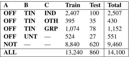
The datasets contain data from Twitter and were provided by the organisers. For Sub-task A, Sub-task B, and Sub-task C, the available datasets (Zampieri et al.,2019a) comprised all the training and testing data. In addition, because the organ-isers did not provide development, we decided to split 0.2 from the training as development. Table 1 shows the data provided by the organisers.

As shown in Table 1, there the data of the three

Sub-tasks shows a significant imbalance.

A B C Train Test Total

OFF TIN IND 2,407 100 2,507

OFF TIN OTH 395 35 430

OFF TIN GRP 1,074 78 1,152

OFF UNT — 524 27 551

NOT — — 8,840 620 9,460

ALL 13,240 860 14,100

Table 1: Distribution of label combinations in the data

3.2 Preprocessing

Initially, we received the training and testing data that had been preprocessed by the organisers. Sub-sequently, on this basis, we preprocessed the train-ing and testtrain-ing data again and finally applied it to a neural network. For preprocessing, we removed and replaced strings from the tweets that did not show any sentiments, irregularities, or abbrevia-tions. We also removed duplicates and Unicode strings. These were implemented as follows:

• Removing consecutive duplicates while re-taining one item: we found that some in-stances of text were duplicates, e.g. ”????”

→”?”.

• Replacing the emojis on Twitter with the cor-responding English definition and replacing abbreviations: There were several emojis in the data conveying different emotions. In ad-dition, the abbreviations in the data also re-strict the corresponding emotional categories, e.g. ”don’t”→”do not”.

• Replacing irregular words: we found that there were many irregular words in the data, e.g. ”bro”→”brother”.

• Removing some punctuation: preliminary experiments showed better results when we removed some punctuation; however, we de-tected emotive punctuation signs such as ”!” and ”?” and retained them.

• Converting lowercase: the final tweets were converted to lowercase (after detecting word-s that had all of their character capitaliword-sed, which were retained).

and Stanford toolkits, we finally decided to use the Stanford toolkit, because of its better performance.

3.3 System

For SemEval-2019 Task 6, we used five basic models:

• BiLSTM: BiLSTM is a combination of for-ward LSTM (LSTM is an artificial recurrent neural network (RNN) architecture; a com-mon LSTM unit comprises a cell, an input gate, an output gate, and a forget gate.) and backward LSTM. Because BiLSTM can bet-ter represent bidirectional semantic depen-dencies, it is often used to model contextual information in natural language processing. In the three Sub-tasks, after several trial com-parisons and time factors, we finally selected a 2-layer BiLSTM. In addition, the parame-ters of our model were chosen to maximise development performance: in Sub-task A, we initialised the hidden dimension, recurrent dropout, and batch size as 120, 0.25, and 128, respectively; in Sub-task B, we initialised the hidden dimension, recurrent dropout, and batch size as 120, 0.25, and 100, respectively; and in Sub-task C, we initialised the hidden dimension, recurrent dropout, and batch size as 140, 0.35, and 64, respectively.

• BiGRU: similarly, BiGRU is a combination of forward GRU (GRU, a variant of LST-M, has a simpler structure than LSTM and works well; there are only two gates in the GRU model, namely the update gate and the reset gate) and backward GRU. For the three Sub-tasks, we used a 2-layer BiGRU. The parameters of our model were chosen to maximise development performance: in Sub-tasks A and B, we initialised the hidden di-mension, recurrent dropout, and batch size as 120, 0.25, and 100, respectively; in Sub-task C, we initialised the hidden dimension, recur-rent dropout, and batch size as 120, 0.25, and 128, respectively.

• BiLSTM with attention: For this, an at-tention layer was added to the 2-layer BiL-STM. In BiLSTM, we used the output vec-tor of the last time sequence as the feature vector and then performed softmax classifi-cation. The attention layer is used to first

calculate the weight of each time sequence, then take the weighted sum of all the time sequence vectors as feature vectors, and fi-nally perform softmax classification. Sim-ilar to the previous models, the parameters of our model were as follows: in Sub-tasks A and B, we initialised the hidden dimen-sion, recurrent dropout, and batch size as 120, 0.25, and 256, respectively; in Sub-task C, we initialised the hidden dimension, recur-rent dropout, and batch size as 180, 0.3, and 128, respectively.

• Capsule Network: In the deep-learning model, the spatial patterns are summarised at the lower level, thus helping represent the concept of higher layers. For example, when a CNN models spatial information, it need-s to copy the feature detector, which reduceneed-s the efficiency of the model. However, spa-tially insensitive methods are inevitably lim-ited by rich text structures (such as the p-reservation of word location information, se-mantic information, and grammatical struc-ture), which are difficult to encode effectively and lack text expression ability. Hinton et al. (Sara Sabour,2017) proposed a Capsule Net-work, which replaces a single neuron node of a traditional neural network with a neu-ron vector and trains this new neural network through dynamic routing, effectively improv-ing the shortcomimprov-ings of the above two meth-ods. The parameters of our model were as follows: in Sub-tasks A and B, we initialised the hidden dimension, batch size, and routing as 64, 120, and 15, respectively; in Sub-task C, we initialised the hidden dimension, batch size, and routing as 64, 140, and 15, respec-tively.

down-stream task model. In other words, it is still utilised when performing downstream tasks, and text classification tasks are natural-ly supported. The model does not need to be modified when performing text classification tasks. The BERT model has two versions on the English datasets, namely Base and Large, and we used the Base version. The param-eters of our model were as follows: trans-former blocks (L) was set as 12, hidden size (H) as 768, number of self-attention head-s (A) ahead-s 12, total parameterhead-s ahead-s 110M, train batch size as 32, predict batch size as 8, and learning rate as 0.00002.

For the four models of BiLSTM, BiGRU, BiL-STM with attention, and Capsule Network, first, the processed Twitter text was converted into a word vector matrix. Then the word vector ma-trix was processed by the embedded layer. Sub-sequently, the word vector matrix was converted to a computable vector matrix. Finally, the four models could utilise the vector matrix for training and prediction.

3.4 K-Fold Cross-Validation

We know from Section 3.1 that data imbalance exists in the public datasets published by the or-ganisers. This would lead to unstable or inaccu-rate experimental results. To manage this problem, we used k-fold (k = 5) cross-validation: the train-ing sample was randomly partitioned into 5 equal sized subsamples. Of the 5 subsamples, a single subsample was retained as validation data to test the model, and the remaining 4 subsamples were used as training data.

4 Results

4.1 Task A

Sub-task A includes 13240 training instances and 860 testing instances, as well as OFF and NOT la-bels. We used four models for predictions on the testing sets. These four models were BERT (sytem ID: 528280), voting (sys(sytem ID: 528117), s-tacking (system ID: 528015), and BiLSTM with attention (system ID: 528232). In the voting mod-el, we performed soft voting ensemble on four ba-sic models: BiLSTM, BiGRU, BiLSTM with at-tention, and Capsule Network. In the stacking model, we performed stacking ensemble on four basic models: BiLSTM, BiGRU, BiLSTM with

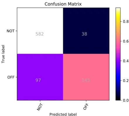
attention, and Capsule Network. Our team results according to those provided by the task organiser-s are organiser-shown in Table 2. Among the reorganiser-sultorganiser-s of the four models submitted by our team, the BiLSTM with attention model performed the best, and its F1 (macro) was 0.7877. The accuracy was 0.843, ranking 16th among all participants. In addition, from the confusion matrix in Figure 1, it is ob-served that when the classifier predicts two classes of labels, namely NOT and OFF, it is more specif-ic to the NOT label, and the precision for the NOT label is higher than that for the OFF label.

System ID F1 (macro) Accuracy

All NOT baseline 0.4189 0.7209 All OFF baseline 0.2182 0.2790 528015 0.7258 0.7872 528117 0.7817 0.836 528280 0.7667 0.8174 528232 0.7877 0.843

Table 2: Results for Sub-task A

NOT OFF

Predicted label NOT

OFF

True label

582

38

97

143

Confusion Matrix

0.0 0.2 0.4 0.6 0.8

Figure 1: Sub-task A, YNU-HPCC CodaLab 528232

4.2 Task B

by our team, the voting model performed best; its F1 (macro) was 0.6811, its accuracy was 0.8625, and it ranked 12th among all participants. Similar to the previous Sub-task, the confusion matrix in Figure 2 indicates that, for the TIN and UNT la-bels, the classifier is more sensitive to TIN labels. In terms of precision, the value for the TIN label is also higher than that for the UNT label.

System ID F1 (macro) Accuracy

All TIN baseline 0.4702 0.8875 All UNT baseline 0.1011 0.1125 533291 0.6811 0.8625 533311 0.6248 0.7833 533313 0.6530 0.8375

Table 3: Results for Sub-task B

TIN _UNT

Predicted label TIN

UNT

True label

194

19

14

13

Confusion Matrix

0.0 0.2 0.4 0.6 0.8

Figure 2: Sub-task B, YNU-HPCC CodaLab 533291

4.3 Task C

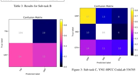
Sub-task C continues on the TIN label of Sub-task B. It includes 3876 training instances and 213 testing instances, as well as IND, OTH, and GRP labels. We used BERT (system ID: 536705) and voting (system ID: 537472) for predictions on the testing sets. The results of our team according to those provided by the task organisers are shown in Table 4. Among the results of the two models submitted by our team, the BERT model performed the best; its F1 (macro) was 0.6212, its accuracy was 0.7089, and it ranked 4th among all participants. Additionally, as shown in Figure 3, among the IND, OTH, and GRP labels, the highest recall and precision are for the IND labels,

and the lowest are for the OTH labels.

For the three Sub-tasks, misclassifications of the classifier are likely due to data imbalance.

System ID F1 (macro) Accuracy

All GRP baseline 0.1787 0.3662 All IND baseline 0.2130 0.4695 All OTH baseline 0.0941 0.1643 536705 0.6212 0.7089 537472 0.5377 0.6667

Table 4: Results for Sub-task C

GRP IND OTH

Predicted label GRP

IND

OTH

True label

57

13

8

10

84

6

14

11

10

Confusion Matrix

0.0 0.1 0.2 0.3 0.4 0.5 0.6 0.7 0.8

Figure 3: Sub-task C, YNU-HPCC CodaLab 536705

5 Conclusion

Acknowledgments

This work was supported by the National Nat-ural Science Foundation of China (NSFC) un-der Grants No.61702443 and No.61762091, and in part by Educational Commission of Yunnan Province of China under Grant No.2017ZZX030. The authors would like to thank the anonymous reviewers and the area chairs for their constructive comments.

References

Christos Doulkeridis Christos Baziotis, Nikos Pelekis. 2017. DataStories at SemEval-2017 Task 4:Deep L-STM with Attention for Message-level and Topic-based Sentiment Analysis. In Proceedings of the 11th International Workshop on Semantic Evalua-tions (SemEval-2017), pages 747–754, Vancouver, Canada.

Thomas Davidson, Dana Warmsley, Michael Macy, and Ingmar Weber. 2017. Automated Hate Speech Detection and the Problem of Offensive Language. InProceedings of ICWSM.

Paula Fortuna and S´ergio Nunes. 2018. A Survey on Automatic Detection of Hate Speech in Text. ACM Computing Surveys (CSUR), 51(4):85.

Bj¨orn Gamb¨ack and Utpal Kumar Sikdar. 2017. Using Convolutional Neural Networks to Classify Hate-speech. In Proceedings of the First Workshop on Abusive Language Online, pages 85–90.

Kenton Lee Kristina Toutanova Jacob Devlin, Ming-Wei Chang. 2018. BERT: Pre-training of Deep Bidi-rectional Transformers for Language Understand-ing. arXiv:1810.04805 [cs.CL].

Tim Salimans Karthik Narasimhan, Alec Radford and Ilya Sutskever. 2018. Improving Language Under-standing by Generative Pre-Training. OpenAI.

Ritesh Kumar, Atul Kr. Ojha, Shervin Malmasi, and Marcos Zampieri. 2018. Benchmarking Aggression Identification in Social Media. InProceedings of the First Workshop on Trolling, Aggression and Cyber-bulling (TRAC), Santa Fe, USA.

Puneet Mathur, Rajiv Shah, Ramit Sawhney, and De-banjan Mahata. 2018. Detecting offensive tweets in hindi-english code-switched language. In Proceed-ings of the 6th International Workshop on Natural Language Processing for Social Media, pages 18– 26.

Matthew E. Peters, Mark Neumann, Mohit Iyyer, Matt Gardner, Christopher Clark, Kenton Lee, and Luke Zettlemoyer. 2018. Deep contextualized word rep-resentations. InProc. of NAACL.

Geoffrey E Hinton Sara Sabour, Nicholas Frosst. 2017. Dynamic Routing Between Capsules. arX-iv:1710.09829 [cs.CV].

John Kordonis Avi Arampatzis Symeon Symeonidis, Dimitrios Effrosynidis. 2017. DUTH at SemEval-2017 Task 4: A Voting Classification Approach for Twitter Sentiment Analysis. InProceedings of the 11th International Workshop on Semantic Evalua-tions (SemEval-2017), pages 704–708, Vancouver, Canada.

Michael Wiegand, Melanie Siegel, and Josef Rup-penhofer. 2018. Overview of the GermEval 2018 Shared Task on the Identification of Offensive Lan-guage. InProceedings of GermEval.

Marcos Zampieri, Shervin Malmasi, Preslav Nakov, Sara Rosenthal, Noura Farra, and Ritesh Kumar. 2019a. Predicting the Type and Target of Offensive Posts in Social Media. InProceedings of NAACL.

Marcos Zampieri, Shervin Malmasi, Preslav Nakov, Sara Rosenthal, Noura Farra, and Ritesh Kumar. 2019b. SemEval-2019 Task 6: Identifying and Cat-egorizing Offensive Language in Social Media (Of-fensEval). InProceedings of The 13th International Workshop on Semantic Evaluation (SemEval).

Ziqi Zhang, David Robinson, and Jonathan Tepper. 2018. Detecting Hate Speech on Twitter Using a Convolution-GRU Based Deep Neural Network. In