Feature Rich Part of Speech Tagging with a Cyclic Dependency Network

Feature-Rich Part-of-Speech Tagging with a Cyclic Dependency Network

Kristina Toutanova

Dan Klein

Computer Science Dept. Computer Science Dept.

Stanford University Stanford University

Stanford, CA 94305-9040 Stanford, CA 94305-9040

[email protected] [email protected]

Christopher D. Manning

Yoram Singer

Computer Science Dept. School of Computer Science

Stanford University The Hebrew University

Stanford, CA 94305-9040 Jerusalem 91904, Israel

[email protected] [email protected]

Abstract

We present a new part-of-speech tagger that demonstrates the following ideas: (i) explicit use of both preceding and following tag con-texts via a dependency network representa-tion, (ii) broad use of lexical features, includ-ing jointly conditioninclud-ing on multiple consecu-tive words, (iii) effecconsecu-tive use of priors in con-ditional loglinear models, and (iv) fine-grained modeling of unknown word features. Using these ideas together, the resulting tagger gives a 97.24% accuracy on the Penn Treebank WSJ, an error reduction of 4.4% on the best previous single automatically learned tagging result.

1

Introduction

Almost all approaches to sequence problems such as part-of-speech tagging take a unidirectional approach to con-ditioning inference along the sequence. Regardless of whether one is using HMMs, maximum entropy condi-tional sequence models, or other techniques like decision trees, most systems work in one direction through the sequence (normally left to right, but occasionally right to left, e.g., Church (1988)). There are a few excep-tions, such as Brill’s transformation-based learning (Brill, 1995), but most of the best known and most successful approaches of recent years have been unidirectional.

Most sequence models can be seen as chaining to-gether the scores or decisions from successive local mod-els to form a global model for an entire sequence. Clearly the identity of a tag is correlated with both past and future tags’ identities. However, in the unidirectional (causal) case, only one direction of influence is explicitly consid-ered at each local point. For example, in a left-to-right

first-order HMM, the current tag t0is predicted based on the previous tag t−1(and the current word).1 The back-ward interaction between t0and the next tag t+1 shows up implicitly later, when t+1is generated in turn. While unidirectional models are therefore able to capture both directions of influence, there are good reasons for sus-pecting that it would be advantageous to make informa-tion from both direcinforma-tions explicitly available for condi-tioning at each local point in the model: (i) because of smoothing and interactions with other modeled features, terms like P(t0|t+1, . . .)might give a sharp estimate of t0 even when terms like P(t+1|t0, . . .)do not, and (ii) jointly considering the left and right context together might be especially revealing. In this paper we exploit this idea, using dependency networks, with a series of local con-ditional loglinear (aka maximum entropy or multiclass logistic regression) models as one way of providing ef-ficient bidirectional inference.

Secondly, while all taggers use lexical information, and, indeed, it is well-known that lexical probabilities are much more revealing than tag sequence probabilities (Charniak et al., 1993), most taggers make quite limited use of lexical probabilities (compared with, for example, the bilexical probabilities commonly used in current sta-tistical parsers). While modern taggers may be more prin-cipled than the classic CLAWS tagger (Marshall, 1987), they are in some respects inferior in their use of lexical information: CLAWS, through its IDIOMTAG module, categorically captured many important, correct taggings of frequent idiomatic word sequences. In this work, we incorporate appropriate multiword feature templates so that such facts can be learned and used automatically by

1_{Rather than subscripting all variables with a position index,}

we use a hopefully clearer relative notation, where t0denotes

the current position and t−nand t+nare left and right context

tags, and similarly for words.

w1 w2 w3 . . . . wn

t1 t2 t3 tn

(a) Left-to-Right CMM

w1 w2 w3 . . . . wn

t1 t2 t3 tn

(b) Right-to-Left CMM

w1 w2 w3 . . . . wn

t1 t2 t3 tn

(c) Bidirectional Dependency Network

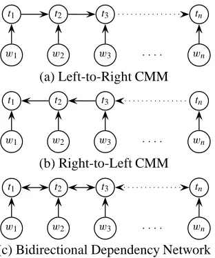
Figure 1: Dependency networks: (a) the (standard) left-to-right first-order CMM, (b) the (reversed) right-to-left CMM, and (c) the bidirectional dependency network.

the model.

Having expressive templates leads to a large number of features, but we show that by suitable use of a prior (i.e., regularization) in the conditional loglinear model – something not used by previous maximum entropy tag-gers – many such features can be added with an overall positive effect on the model. Indeed, as for the voted per-ceptron of Collins (2002), we can get performance gains by reducing the support threshold for features to be in-cluded in the model. Combining all these ideas, together with a few additional handcrafted unknown word fea-tures, gives us a part-of-speech tagger with a per-position tag accuracy of 97.24%, and a whole-sentence correct rate of 56.34% on Penn Treebank WSJ data. This is the best automatically learned part-of-speech tagging result known to us, representing an error reduction of 4.4% on the model presented in Collins (2002), using the same data splits, and a larger error reduction of 12.1% from the more similar best previous loglinear model in Toutanova and Manning (2000).

2

Bidirectional Dependency Networks

When building probabilistic models for tag sequences, we often decompose the global probability of sequences using a directed graphical model (e.g., an HMM (Brants, 2000) or a conditional Markov model (CMM) (Ratna-parkhi, 1996)). In such models, the probability assigned to a tagged sequence of words x = ht, wiis the product of a sequence of local portions of the graphical model, one from each time slice. For example, in the left-to-right CMM shown in figure 1(a),

P(t, w)=Y

iP(ti|ti−1, wi)

That is, the replicated structure is a local model

P(t0|t−1, w0).2 Of course, if there are too many con-ditioned quantities, these local models may have to be estimated in some sophisticated way; it is typical in tag-ging to populate these models with little maximum en-tropy models. For example, we might populate a model for P(t0|t−1, w0)with a maxent model of the form:

Pλ(t0|t−1, w0)=

exp(λht0,t−1i+λht0,w0i) P

t0

0exp(λht

0

0,t−1i+λht00,w0i)

In this case, thew0and t−1can have joint effects on t0, but there are not joint features involving all three variables (though there could have been such features). We say that this model uses the feature templatesht0,t−1i(previous tag features) andht0, w0i(current word features).

Clearly, both the preceding tag t−1 and following tag t+1carry useful information about a current tag t0. Unidi-rectional models do not ignore this influence; in the case of a left-to-right CMM, the influence of t−1 on t0 is ex-plicit in the P(t0|t−1, w0)local model, while the influ-ence of t+1on t0is implicit in the local model at the next position (via P(t+1|t0, w+1)). The situation is reversed

for the right-to-left CMM in figure 1(b).

From a seat-of-the-pants machine learning perspective, when building a classifier to label the tag at a certain posi-tion, the obvious thing to do is to explicitly include in the local model all predictive features, no matter on which side of the target position they lie. There are two good formal reasons to expect that a model explicitly condi-tioning on both sides at each position, like figure 1(c) could be advantageous. First, because of smoothing effects and interaction with other conditioning features (like the words), left-to-right factors like P(t0|t−1, w0) do not always suffice when t0is implicitly needed to de-termine t−1. For example, consider a case of observation bias (Klein and Manning, 2002) for a first-order left-to-right CMM. The word to has only one tag (TO) in the PTB tag set. TheTOtag is often preceded by nouns, but rarely by modals (MD). In a sequence will to fight, that trend indicates that will should be a noun rather than a modal verb. However, that effect is completely lost in a CMM like (a): P(twill|will,hstar ti)prefers the modal tagging, and P(TO|to,twill)is roughly 1 regardless of twill. While the model has an arrow between the two tag positions, that path of influence is severed.3 The same problem ex-ists in the other direction. If we use the symmetric

right-2_{Throughout this paper we assume that enough boundary}

symbols always exist that we can ignore the differences which would otherwise exist at the initial and final few positions.

3_{Despite use of names like “label bias” (Lafferty et al., 2001)}

A B A B A B

(a) (b) (c)

Figure 2: Simple dependency nets: (a) the Bayes’ net for

P(A)P(B|A), (b) the Bayes’ net for P(A|B)P(B), (c) a bidi-rectional net with models of P(A|B)and P(B|A), which is not a Bayes’ net.

to-left model, fight will receive its more common noun tagging by symmetric reasoning. However, the bidirec-tional model (c) discussed in the next section makes both directions available for conditioning at all locations, us-ing replicated models of P(t0|t−1,t+1, w0), and will be able to get this example correct.4

2.1 Semantics of Dependency Networks

While the structures in figure 1(a) and (b) are well-understood graphical models with well-known semantics, figure 1(c) is not a standard Bayes’ net, precisely because the graph has cycles. Rather, it is a more general

de-pendency network (Heckerman et al., 2000). Each node

represents a random variable along with a local condi-tional probability model of that variable, conditioned on the source variables of all incoming arcs. In this sense, the semantics are the same as for standard Bayes’ nets. However, because the graph is cyclic, the net does not correspond to a proper factorization of a large joint prob-ability estimate into local conditional factors. Consider the two-node cases shown in figure 2. Formally, for the net in (a), we can write P(a,b)= P(a)P(b|a). For (b) we write P(a,b) = P(b)P(a|b). However, in (c), the nodes A and B carry the information P(a|b)and P(b|a) respectively. The chain rule doesn’t allow us to recon-struct P(a,b)by multiplying these two quantities. Un-der appropriate conditions, we could reconstruct P(a,b) from these quantities using Gibbs sampling, and, in gen-eral, that is the best we can do. However, while recon-structing the joint probabilities from these local condi-tional probabilities may be difficult, estimating the local probabilities themselves is no harder than it is for acyclic models: we take observations of the local environments and use any maximum likelihood estimation method we desire. In our experiments, we used local maxent models, but if the event space allowed, (smoothed) relative counts would do.

4_{The effect of indirect influence being weaker than direct}

in-fluence is more pronounced for conditionally structured models, but is potentially an issue even with a simple HMM. The prob-abilistic models for basic left-to-right and right-to-left HMMs with emissions on their states can be shown to be equivalent us-ing Bayes’ rule on the transitions, provided start and end sym-bols are modeled. However, this equivalence is violated in prac-tice by the addition of smoothing.

function bestScore()

return bestScoreSub(n+2,hend,end,endi);

function bestScoreSub(i+1,hti−1,ti,ti+1i)

% memoization

if (cached(i+1,hti−1,ti,ti+1i))

return cache(i+1,hti−1,ti,ti+1i);

% left boundary case if (i= −1)

if (hti−1,ti,ti+1i == hst ar t,st ar t,st ar ti)

return 1; else

return 0; % recursive case

return maxti−2 bestScoreSub(i,hti−2,ti−1,tii)× P(ti|ti−1,ti+1, wi);

Figure 3: Pseudocode for polynomial inference for the first-order bidirectional CMM (memoized version).

2.2 Inference for Linear Dependency Networks

Cyclic or not, we can view the product of local probabil-ities from a dependency network as a score:

scor e(x)=Y

iP(xi|Pa(xi))

where Pa(xi)are the nodes with arcs to the node xi. In the case of an acyclic model, this score will be the joint prob-ability of the event x , P(x). In the general case, it will not be. However, we can still ask for the event, in this case the tag sequence, with the highest score. For dependency net-works like those in figure 1, an adaptation of the Viterbi algorithm can be used to find the maximizing sequence in polynomial time. Figure 3 gives pseudocode for the concrete case of the network in figure 1(d); the general case is similar, and is in fact just a max-plus version of standard inference algorithms for Bayes’ nets (Cowell et al., 1999, 97). In essence, there is no difference between inference on this network and a second-order left-to-right CMM or HMM. The only difference is that, when the Markov window is at a position i , rather than receiving the score for P(ti|ti−1,ti−2, wi), one receives the score for P(ti−1|ti,ti−2, wi−1).

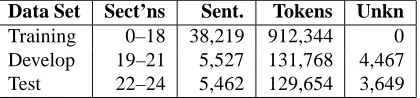
Data Set Sect’ns Sent. Tokens Unkn

Training 0–18 38,219 912,344 0

Develop 19–21 5,527 131,768 4,467

Test 22–24 5,462 129,654 3,649

Table 1: Data set splits used.

above. Consider the following training set, for the same network, with each entire data point considered as a label:

h11,22i. The relative-frequency model assigns loss 0 to both training examples, but cannot do better than 50% error in regenerating the training data labels. These is-sues are further discussed in Heckerman et al. (2000). Preliminary work of ours suggests that practical use of dependency networks is not in general immune to these theoretical concerns: a dependency network can choose a sequence model that is bidirectionally very consistent but does not match the data very well. However, this problem does not appear to have prevented the networks from per-forming well on the tagging problem, probably because features linking tags and observations are generally much sharper discriminators than tag sequence features.

It is useful to contrast this framework with the con-ditional random fields of Lafferty et al. (2001). The CRF approach uses similar local features, but rather than chaining together local models, they construct a sin-gle, globally normalized model. The principal tage of the dependency network approach is that advan-tageous bidirectional effects can be obtained without the extremely expensive global training required for CRFs.

To summarize, we draw a dependency network in which each node has as neighbors all the other nodes that we would like to have influence it directly. Each node’s neighborhood is then considered in isolation and a local model is trained to maximize the conditional like-lihood over the training data of that node. At test time, the sequence with the highest product of local conditional scores is calculated and returned. We can always find the exact maximizing sequence, but only in the case of an acyclic net is it guaranteed to be the maximum likelihood sequence.

3

Experiments

The part of speech tagged data used in our experiments is the Wall Street Journal data from Penn Treebank III (Mar-cus et al., 1994). We extracted tagged sentences from the parse trees.5We split the data into training, development, and test sets as in (Collins, 2002). Table 1 lists

character-5_{Note that these tags (and sentences) are not identical to}

those obtained from thetagged/posdirectories of the same disk: hundreds of tags in the RB/RP/IN set were changed to be more consistent in theparsed/mrgversion. Maybe we were the last to discover this, but we’ve never seen it in print.

istics of the three splits.6 Except where indicated for the modelBEST, all results are on the development set.

One innovation in our reporting of results is that we present whole-sentence accuracy numbers as well as the traditional per-tag accuracy measure (over all tokens, even unambiguous ones). This is the quantity that most sequence models attempt to maximize (and has been mo-tivated over doing per-state optimization as being more useful for subsequent linguistic processing: one wants to find a coherent sentence interpretation). Further, while some tag errors matter much more than others, to a first cut getting a single tag wrong in many of the more com-mon ways (e.g., proper noun vs. comcom-mon noun; noun vs. verb) would lead to errors in a subsequent processor such as an information extraction system or a parser that would greatly degrade results for the entire sentence. Finally, the fact that the measure has much more dynamic range has some appeal when reporting tagging results.

The per-state models in this paper are log-linear mod-els, building upon the models in (Ratnaparkhi, 1996) and (Toutanova and Manning, 2000), though some models are in fact strictly simpler. The features in the models are defined using templates; there are different templates for rare words aimed at learning the correct tags for unknown words.7We present the results of three classes of experi-ments: experiments with directionality, experiments with lexicalization, and experiments with smoothing.

3.1 Experiments with Directionality

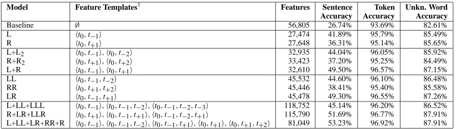
In this section, we report experiments using log-linear CMMs to populate nets with various structures, exploring the relative value of neighboring words’ tags. Table 2 lists the discussed networks. All networks have the same ver-tical feature templates:ht0, w0ifeatures for known words and variousht0, σ (w1n)iword signature features for all words, known or not, including spelling and capitaliza-tion features (see seccapitaliza-tion 3.3).

Just this vertical conditioning gives an accuracy of 93.69% (denoted as “Baseline” in table 2).8

Condition-6_{Tagger results are only comparable when tested not only on}

the same data and tag set, but with the same amount of training data. Brants (2000) illustrates very clearly how tagging perfor-mance increases as training set size grows, largely because the percentage of unknown words decreases while system perfor-mance on them increases (they become increasingly restricted as to word class).

7_{Except where otherwise stated, a count cutoff of 2 was used}

for common word features and 35 for rare word features (tem-plates need a support set strictly greater in size than the cutoff before they are included in the model).

8_{Charniak et al. (1993) noted that such a simple model got}

base-Model Feature Templates† Features Sentence Token Unkn. Word

Accuracy Accuracy Accuracy

Baseline ∅ 56,805 26.74% 93.69% 82.61%

L ht0,t−1i 27,474 41.89% 95.79% 85.49%

R ht0,t+1i 27,648 36.31% 95.14% 85.65%

L+L2 ht0,t−1i,ht0,t−2i 32,935 44.04% 96.05% 85.92% R+R2 ht0,t+1i,ht0,t+2i 33,423 37.20% 95.25% 84.49% L+R ht0,t−1i,ht0,t+1i 32,610 49.50% 96.57% 87.15%

LL ht0,t−1,t−2i 45,532 44.60% 96.10% 86.48%

RR ht0,t+1,t+2i 45,446 38.41% 95.40% 85.58%

LR ht0,t−1,t+1i 45,478 49.30% 96.55% 87.26%

L+LL+LLL ht0,t−1i,ht0,t−1,t−2i,ht0,t−1,t−2,t−3i 118,752 45.14% 96.20% 86.52% R+LR+LLR ht0,t+1i,ht0,t−1,t+1i,ht0,t−1,t−2,t+1i 115,790 51.69% 96.77% 87.91% L+LL+LR+RR+R ht0,t−1i,ht0,t−1,t−2i,ht0,t−1,t+1i,ht0,t+1i,ht0,t+1,t+2i 81,049 53.23% 96.92% 87.91%

Table 2: Tagging accuracy on the development set with different sequence feature templates. †All models include the same vertical word-tag features (ht0, w0iand variousht0, σ (w1n)i), though the baseline uses a lower cutoff for these features.

Model Feature Templates Support Features Sentence Token Unknown

Cutoff Accuracy Accuracy Accuracy

BASELINE ht₀, w0i 2 6,501 1.63% 60.16% 82.98%

ht₀, w0i 0 56,805 26.74% 93.69% 82.61%

3W ht0, w0i,ht0, w−1i,ht0, w+1i 2 239,767 48.27% 96.57% 86.78%

3W+TAGS tag sequences,ht0, w0i,ht0, w−1i,ht0, w+1i 2 263,160 53.83% 97.02% 88.05%

BEST see text 2 460,552 55.31% 97.15% 88.61%

Table 3: Tagging accuracy with different lexical feature templates on the development set.

Model Feature Templates Support Features Sentence Token Unknown

Cutoff Accuracy Accuracy Accuracy

BEST see text 2 460,552 56.34% 97.24% 89.04%

Table 4: Final tagging accuracy for the best model on the test set.

ing on the previous tag as well (model L,ht0,t−1i fea-tures) gives 95.79%. The reverse, model R, using the next tag instead, is slightly inferior at 95.14%. Model L+R, using both tags simultaneously (but with only the individual-direction features) gives a much better accu-racy of 96.57%. Since this model has roughly twice as many tag-tag features, the fact that it outperforms the uni-directional models is not by itself compelling evidence for using bidirectional networks. However, it also out-performs model L+L2 which adds the ht0,t−2i second-previous word features instead of next word features, which gives only 96.05% (and R+R2gives 95.25%). We conclude that, if one wishes to condition on two neigh-boring nodes (using two sets of 2-tag features), the sym-metric bidirectional model is superior.

High-performance taggers typically also include joint three-tag counts in some way, either as tag trigrams (Brants, 2000) or tag-triple features (Ratnaparkhi, 1996, Toutanova and Manning, 2000). Models LL, RR, and CR use only the vertical features and a single set of tag-triple features: the left tags (t−2, t−1and t0), right tags (t0, t+1, t+2), or centered tags (t−1, t0, t+1) respectively. Again, with roughly equivalent feature sets, the left context is better than the right, and the centered context is better than either unidirectional context.

line for this task high, while substantial annotator noise creates an unknown upper bound on the task.

3.2 Lexicalization

Lexicalization has been a key factor in the advance of statistical parsing models, but has been less exploited for tagging. Words surrounding the current word have been occasionally used in taggers, such as (Ratnaparkhi, 1996), Brill’s transformation based tagger (Brill, 1995), and the HMM model of Lee et al. (2000), but neverthe-less, the only lexicalization consistently included in tag-ging models is the dependence of the part of speech tag of a word on the word itself.

In maximum entropy models, joint features which look at surrounding words and their tags, as well as joint fea-tures of the current word and surrounding words are in principle straightforward additions, but have not been in-corporated into previous models. We have found these features to be very useful. We explore here lexicaliza-tion both alone and in combinalexicaliza-tion with preceding and following tag histories.

The third row shows a model where a tag is de-cided solely by the three words centered at the tag po-sition (3W). As far as we are aware, models of this sort have not been explored previously, but its accu-racy is surprisingly high: despite having no sequence model at all, it is more accurate than a model which uses standard tag fourgram HMM features (ht0, w0i,ht0,t−1i, ht0,t−1,t−2i,ht0,t−1,t−2,t−3i, shown in Table 2, model L+LL+LLL).

The fourth and fifth rows show models with bi-directional tagging features. The fourth model (3W+TAGS) uses the same tag sequence features as the last model in Table 2 (ht0,t−1i,ht0,t−1,t−2i, ht0,t−1,t+1i,ht0,t+1i,ht0,t+1,t+2i) and current, previ-ous, and next word. The last model has in ad-dition the feature templates ht0, w0,t−1i,ht0, w0,t+1i, ht0, w−1, w0i, and ht0, w0, w+1i, and includes the im-provements in unknown word modeling discussed in sec-tion 3.3.9 We call this model BEST. BEST has a to-ken accuracy on the final test set of 97.24% and a sen-tence accuracy of 56.34% (see Table 4). A 95% confi-dence interval for the accuracy (using a binomial model) is(97.15%,97.33%).

In order to understand the gains from using right con-text tags and more lexicalization, let us look at an exam-ple of an error that the enriched models learn not to make. An interesting example of a common tagging error of the simpler models which could be corrected by a determinis-tic fixup rule of the kind used in the IDIOMTAG module of (Marshall, 1987) is the expression as X as (often, as

far as). This should be tagged as/RB X/{RB,JJ}as/IN in

the Penn Treebank. A model using only current word and two left tags (model L+L2in Table 2), made 87 errors on this expression, tagging it as/IN X as/IN – since the tag sequence probabilities do not give strong reasons to dis-prefer the most common tagging of as (it is tagged as IN over 80% of the time). However, the model 3W+TAGS, which uses two right tags and the two surrounding words in addition, made only 8 errors of this kind, and model BESTmade only 6 errors.

3.3 Unknown word features

Most of the models presented here use a set of un-known word features basically inherited from (Ratna-parkhi, 1996), which include using character n-gram pre-fixes and sufpre-fixes (for n up to 4), and detectors for a few other prominent features of words, such as capitaliza-tion, hyphens, and numbers. Doing error analysis on un-known words on a simple tagging model (withht0,t−1i, ht0,t−1,t−2i, andhw0,t0ifeatures) suggested several ad-ditional specialized features that can usefully improve

9_{Thede and Harper (1999) use ht}

−1,t0, w0itemplates in

their “full-second order” HMM, achieving an accuracy of 96.86%. Here we can add the opposite tiling and other features.

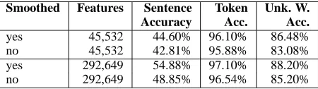
Smoothed Features Sentence Token Unk. W.

Accuracy Acc. Acc.

yes 45,532 44.60% 96.10% 86.48% no 45,532 42.81% 95.88% 83.08% yes 292,649 54.88% 97.10% 88.20% no 292,649 48.85% 96.54% 85.20%

Table 5: Accuracy with and without quadratic regularization.

performance. By far the most significant is a crude com-pany name detector which marks capitalized words fol-lowed within 3 words by a company name suffix like Co. or Inc. This suggests that further gains could be made by incorporating a good named entity recognizer as a prepro-cessor to the tagger (reversing the most common order of processing in pipelined systems!), and is a good example of something that can only be done when using a condi-tional model. Minor gains come from a few addicondi-tional features: an allcaps feature, and a conjunction feature of words that are capitalized and have a digit and a dash in them (such words are normally common nouns, such as

CFC-12 or F/A-18). We also found it advantageous to

use prefixes and suffixes of length up to 10. Together with the larger templates, these features contribute to our unknown word accuracies being higher than those of pre-viously reported taggers.

3.4 Smoothing

With so many features in the model, overtraining is a dis-tinct possibility when using pure maximum likelihood es-timation. We avoid this by using a Gaussian prior (aka quadratic regularization or quadratic penalization) which resists high feature weights unless they produce great score gain. The regularized objective F is:

F(λ₎=X

ilog(Pλ(ti|w,t))+

Xn

j=1 λ2_j

2σ2

Since we use a conjugate-gradient procedure to maximize the data likelihood, the addition of a penalty term is eas-ily incorporated. Both the total size of the penalty and the partial derivatives with repsect to each λj are triv-ial to compute; these are added to the log-likelihood and log-likelihood derivatives, and the penalized optimization procedes without further modification.

We have not extensively experimented with the value ofσ2– which can even be set differently for different pa-rameters or parameter classes. All the results in this paper use a constantσ2= 0.5, so that the denominator disap-pears in the above expression. Experiments on a simple model withσmade an order of magnitude higher or lower both resulted in worse performance than withσ2=0.5.

Tagger Support cutoff Accuracy Collins (2002) 0 96.60% 5 96.72% Model 3W+TAGSvariant 1 96.97% 5 96.93%

Table 6: Effect of changing common word feature cutoffs (fea-tures with support≤cutoff are excluded from the model).

number of features used in our complex models – in the several hundreds of thousands, is extremely high in com-parison with the data set size and the number of features used in other machine learning domains. We describe two sets of experiments aimed at comparing models with and without regularization. One is for a simple model with a relatively small number of features, and the other is for a model with a large number of features.

The usefulness of priors in maximum entropy models is not new to this work: Gaussian prior smoothing is ad-vocated in Chen and Rosenfeld (2000), and used in all the stochastic LFG work (Johnson et al., 1999). How-ever, until recently, its role and importance have not been widely understood. For example, Zhang and Oles (2001) attribute the perceived limited success of logistic regres-sion for text categorization to a lack of use of regular-ization. At any rate, regularized conditional loglinear models have not previously been applied to the prob-lem of producing a high quality part-of-speech tagger: Ratnaparkhi (1996), Toutanova and Manning (2000), and Collins (2002) all present unregularized models. Indeed, the result of Collins (2002) that including low support features helps a voted perceptron model but harms a max-imum entropy model is undone once the weights of the maximum entropy model are regularized.

Table 5 shows results on the development set from two pairs of experiments. The first pair of models use com-mon word templatesht0, w0i,ht0,t−1,t−2iand the same rare word templates as used in the models in table 2. The second pair of models use the same features as model BEST with a higher frequency cutoff of 5 for common word features.

For the first pair of models, the error reduction from smoothing is 5.3% overall and 20.1% on unknown words. For the second pair of models, the error reduction is even bigger: 16.2% overall after convergence and 5.8% if looking at the best accuracy achieved by the unsmoothed model (by stopping training after 75 iterations; see be-low). The especially large reduction in unknown word er-ror reflects the fact that, because penalties are effectively stronger for rare features than frequent ones, the presence of penalties increases the degree to which more general cross-word signature features (which apply to unknown words) are used, relative to word-specific sparse features (which do not apply to unknown words).

Secondly, use of regularization allows us to incorporate features with low support into the model while improving

96,3 96,4 96,5 96,6 96,7 96,8 96,9 97 97,1 97,2

0 100 200 300 400

Training Iterations

Accuracy

No Smoothing Smoothing

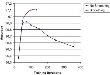
Figure 4: Accuracy by training iterations, with and without quadratic regularization.

performance. Whereas Ratnaparkhi (1996) used feature support cutoffs and early stopping to stop overfitting of the model, and Collins (2002) contends that including low support features harms a maximum entropy model, our results show that low support features are useful in a regularized maximum entropy model. Table 6 contrasts our results with those from Collins (2002). Since the models are not the same, the exact numbers are incompa-rable, but the difference in direction is important: in the regularized model, performance improves with the inclu-sion of low support features.

Finally, in addition to being significantly more accu-rate, smoothed models train much faster than unsmoothed ones, and do not benefit from early stopping. For ex-ample, the first smoothed model in Table 5 required 80 conjugate gradient iterations to converge (somewhat ar-bitrarily defined as a maximum difference of 10−4in fea-ture weights between iterations), while its corresponding unsmoothed model required 335 iterations, thus training was roughly 4 times slower.10The second pair of models required 134 and 370 iterations respectively. As might be expected, unsmoothed models reach their highest gen-eralization capacity long before convergence and accu-racy on an unseen test set drops considerably with fur-ther iterations. This is not the case for smoothed mod-els, as their test set accuracy increases almost monoton-ically with training iterations.11 Figure 4 shows a graph of training iterations versus accuracy for the second pair of models on the development set.

4

Conclusion

We have shown how broad feature use, when combined with appropriate model regularization, produces a supe-rior level of tagger performance. While experience

sug-10_{On a 2GHz PC, this is still an important difference: our}

largest models require about 25 minutes per iteration to train.

11_{In practice one notices some wiggling in the curve, but}

gests that the final accuracy number presented here could be slightly improved upon by classifier combination, it is worth noting that not only is this tagger better than any previous single tagger, but it also appears to outperform Brill and Wu (1998), the best-known combination tagger (they report an accuracy of 97.16% over the same WSJ data, but using a larger training set, which should favor them).

While part-of-speech tagging is now a fairly well-worn road, and our ability to win performance increases in this domain is starting to be limited by the rate of er-rors and inconsistencies in the Penn Treebank training data, this work also has broader implications. Across the many NLP problems which involve sequence mod-els over sparse multinomial distributions, it suggests that feature-rich models with extensive lexicalization, bidirec-tional inference, and effective regularization will be key elements in producing state-of-the-art results.

Acknowledgements

This work was supported in part by the Advanced Re-search and Development Activity (ARDA)’s Advanced Question Answering for Intelligence (AQUAINT) Pro-gram, by the National Science Foundation under Grant No. IIS-0085896, and by an IBM Faculty Partnership Award.

References

Steven Abney, Robert E. Schapire, and Yoram Singer. 1999. Boosting applied to tagging and PP attachment. In

EMNLP/VLC 1999, pages 38–45.

Thorsten Brants. 2000. TnT – a statistical part-of-speech tagger. In ANLP 6, pages 224–231.

Eric Brill and Jun Wu. 1998. Classifier combination for improved lexical disambiguation. In ACL 36/COLING 17, pages 191–195.

Eric Brill. 1995. Transformation-based error-driven learning and natural language processing: A case study in part-of-speech tagging. Computational Linguistics, 21(4):543–565. Eugene Charniak, Curtis Hendrickson, Neil Jacobson, and Mike

Perkowitz. 1993. Equations for part-of-speech tagging. In

AAAI 11, pages 784–789.

Stanley F. Chen and Ronald Rosenfeld. 2000. A survey of smoothing techniques for maximum entropy models. IEEE

Transactions on Speech and Audio Processing, 8(1):37–50.

Kenneth W. Church. 1988. A stochastic parts program and noun phrase parser for unrestricted text. In ANLP 2, pages 136–143.

Michael Collins. 2002. Discriminative training methods for Hidden Markov Models: Theory and experiments with per-ceptron algorithms. In EMNLP 2002.

Robert G. Cowell, A. Philip Dawid, Steffen L. Lauritzen, and David J. Spiegelhalter. 1999. Probabilistic Networks and

Expert Systems. Springer-Verlag, New York.

David Heckerman, David Maxwell Chickering, Christopher Meek, Robert Rounthwaite, and Carl Myers Kadie. 2000. Dependency networks for inference, collaborative filtering and data visualization. Journal of Machine Learning

Re-search, 1(1):49–75.

Mark Johnson, Stuart Geman, Stephen Canon, Zhiyi Chi, and Stefan Riezler. 1999. Estimators for stochastic “unification-based” grammars. In ACL 37, pages 535–541.

Dan Klein and Christopher D. Manning. 2002. Conditional structure versus conditional estimation in NLP models. In

EMNLP 2002, pages 9–16.

John Lafferty, Andrew McCallum, and Fernando Pereira. 2001. Conditional random fields: Probabilistic models for seg-menting and labeling sequence data. In ICML-2001, pages 282–289.

Sang-Zoo Lee, Jun ichi Tsujii, and Hae-Chang Rim. 2000. Part-of-speech tagging based on Hidden Markov Model assuming joint independence. In ACL 38, pages 263–169.

Mitchell P. Marcus, Beatrice Santorini, and Mary A. Marcinkie-wicz. 1994. Building a large annotated corpus of English: The Penn Treebank. Computational Linguistics, 19:313–

330.

Ian Marshall. 1987. Tag selection using probabilistic methods. In Roger Garside, Geoffrey Sampson, and Geoffrey Leech, editors, The Computational analysis of English: a

corpus-based approach, pages 42–65. Longman, London.

Adwait Ratnaparkhi. 1996. A maximum entropy model for part-of-speech tagging. In EMNLP 1, pages 133–142. Scott M. Thede and Mary P. Harper. 1999. Second-order hidden

Markov model for part-of-speech tagging. In ACL 37, pages 175–182.

Kristina Toutanova and Christopher Manning. 2000. Enriching the knowledge sources used in a maximum entropy part-of-speech tagger. In EMNLP/VLC 1999, pages 63–71. Tong Zhang and Frank J. Oles. 2001. Text categorization based

on regularized linear classification methods. Information