Words are Vectors, Dependencies are Matrices: Learning Word
Embeddings from Dependency Graphs
Paula Czarnowska, Guy Emerson and Ann Copestake Department of Computer Science and Technology
University of Cambridge
{pjc211, gete2, aac10}@cam.ac.uk
Abstract
Distributional Semantic Models (DSMs) construct vector representations of word meanings based on their contexts. Typically, the contexts of a word are defined as its closest neighbours, but they can also be retrieved from its syntactic dependency relations. In this work, we propose a new dependency-based DSM. The novelty of our model lies in associating an independent meaning representation, a matrix, with each dependency-label. This allows it to capture specifics of the relations between words and contexts, leading to good performance on both intrinsic and extrinsic evaluation tasks. In addi-tion to that, our model has an inherent ability to represent dependency chains as products of matrices which provides a straightforward way of handling further contexts of a word.
1
Introduction
Within computational linguistics, most research on word-meaning has been focusing on developing Dis-tributional Semantic Models (DSMs), based on the hypothesis that a word’s sense can be inferred from the contexts it appears in (Harris, 1954). DSMs associate each word with a vector (a.k.a.word embed-ding) that encodes information about its co-occurrence with other words in the vocabulary. In recent work, the most popular DSMs learn the embeddings using neural-network architectures. In particular, the Skip-gram model of Mikolov et al. (2013) has gained a lot of traction due to its efficiency and high quality representations. Skip-gram embeddings are trained with an objective that forces them to be sim-ilar to the vectors of their words’ contexts. The latter, context-word vectors, are a separate parameter of the model jointly learned along with the maintarget-wordvectors. Like most DSMs, Mikolov et al. (2013)’s model derives contexts of a word from a pre-defined window of words that surround it.
An alternative way of defining contexts in Skip-gram was explored by Levy and Goldberg (2014), who altered the model to accept contexts coming from a different vocabulary to that of the target-words. The contexts were retrieved from targets’ syntactic dependency relations and were a concatenation of the word linked to the target and the dependency-label. Each context type was associated with an indepen-dent vector representation. In contrast to Skip-gram, which captures relatedness1, Levy and Goldberg (2014)’s embeddings exhibited a more intuitive notion of similarity. For example, the former regards the vector forabba, a popular Swedish pop group, as close to that foragnetha– a name of the group’s mem-ber, while the latter considers it close to the vectors for other pop group names. But Levy and Goldberg (2014)’s method of constructing contexts prevented their model from directly capturing how dependency types affect relations between target and context-words, as the labels were not associated with indepen-dent representations. At the same time it intensifies the problems associated with data sparsity due to the large and fine-grained context-vocabulary.
In this work, we address the shortcomings of Levy and Goldberg (2014)’s approach by introducing thedependency-matrix model– a DSM which associates meaning with each type of dependency. Instead
1Turney (2012) refers to relatedness as
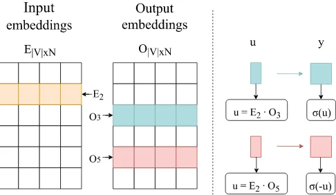
Figure 1: A graphical representation of Skip-gram displaying its parameters (left) and how P(C = 1|V2, V3)and1−P(C = 1|V2, V5)are calculated for the real and a negative context, respectively. N is
the embedding dimensionality.
of simply appending the labels to context-words, they are promoted to a separate parameter of the model. They become matrices, acting as linear maps on the context-word vectors and trained alongside the em-beddings. We hypothesised that this approach will lead to higher-quality representations, as it allows the model to capture important interactions between all three: labels, contexts and targets, while diminishing the data sparsity problem at the same time.
2
Background
2.1 The Skip-gram Model
We now give a short formal overview of the Skip-gram model, since we will build on this to specify our dependency-matrix model in Section 3.
Skip-gram was based on the feed-forward neural probabilistic language model of Bengio et al. (2003). It is trained to predict the context-words of a given target-word, where the contexts are the immediate neighbours of the latter and are retrieved using a window of an arbitrary sizen(by capturing nwords to the left of the target andnwords to its right). During training the model is exposed to vast amounts of training data pairs (Vt,Vc), whereV is the vocabulary andt, c ∈ {1, ...,|V|}are indices of a target-word and one of its contexts. The objective of negative-sampling Skip-gram, as introduced by Mikolov et al. (2013), is to differentiate between the correct training examples retrieved from the corpus and the incorrect, randomly generated pairs. For each correct example the model drawsmnegative ones, withm being a hyperparameter. These incorrect samples hold the sameVtas the original, while their Vc is drawn from an arbitrary noise distribution. Mikolov et al. (2013) recommend setting the noise distribution to the unigram distribution raised to the power0.75and we used this setting in this work.
Following Goldberg and Levy (2014), let Dbe the set of all correct pairs, D0 denote a set of all negatively sampled|D| ×m pairs andP(C = 1|Vt, Vc) be the probability of (Vt, Vc) being a correct pair, originating from the corpus. The last is calculated using the sigmoid function:
σ(u) = 1
1 +e−u (1)
where u=Et·Oc
Here,E ∈ R|V|×N stands for aninput-embeddingmatrix, holding representations of target-words and O ∈ R|V|×N stands for the output-embeddingmatrix, holding context representations (see Figure 1).
Given this setting, the negative-sampling objective is defined as maximising
X
(Vt,Vc)∈D
log σ(u) + X
(Vt,Vc)∈D0
The model is trained using stochastic gradient ascent, with the learning rate changing throughout the training process and being proportional to the number of remaining training examples.
2.2 Dependency-based Embeddings
Since word meaning is closely related to syntactic behaviour, a feasible alternative to the window-method is to extract the contexts from the word’s syntactic relations. This can be achieved by constructing the context vocabulary VC through pairing all word types with labels of relations they can participate in. For instance, among the contexts composed fromdogwould bedog/nsubjanddog/dobj. Alternatively, one can keep the vocabulary unchanged and adjust the context selection method to disregard the labels and only pick words in relation with the target. The first approach was taken in some of the earliest works incorporating syntactic information into the count-based DSMs. Grefenstette (1994) used VC that consists of tokens such as subject-of-talkand his vectors held binary values denoting whether the target-word has co-occurred with the contexts inVC. This approach was later extended by Lin (1998) who replaced the binary values with frequency counts. Even more methods for incorporating syntactic information were introduced in the general frameworks of Pad´o and Lapata (2007)’s and Baroni and Lenci (2010). Baroni and Lenci (2010) represented corpus-extracted frequencies of (word, link, word) tuples as a third order tensor and, through its matricisation, generated various matrix-arrangements of the data. In particular, as an alternative to the standardword by (link, word)matrix, the framework allows the focus to be placed on links (which can be dependencies) and represent them in terms of the words they connect through alink by (word, word)matrix.
More recently, Levy and Goldberg (2014) modified Skip-gram to use contexts of the form context-word’s form/label. The context-word can be either the head or a modifier of the target, with the first role causing the dependency to be marked asinverse. For example, if we take the sentence‘I like rain’:
I like rain.
nsubj dobj
forrainwe obtainlike/dobj−1context, marked with−1to reflect the relation’s inverse nature.
One weaker side of this model is that it does not directly capture how the dependency type affects the relation between the head and the dependent. For instance, during training it does not recognise that thensubjdependency in both sentences
Harry danced. Kate laughed.
nsubj nsubj
is in fact a relation of the very same type and cannot make use of the available subjecthood information – a good indicator of words’ agentivity or animacy. In fact, it does not provide any mechanisms for indicating that the contextsdanced/nsubj−1 andlaughed/nsubj−1 have anything in common, apart from the fact that they will likely be contexts of similar words. Naturally, the latter is strongly informative in its own right, but associating meaning with specific types of dependencies could further improve the model’s performance. One benefit of such a solution is the increased informativeness of rare context-words in cases when they appear in common relations.
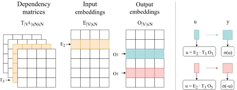
Figure 2: A representation of our model displaying its parameters (left) and howP(C = 1|V2, V3, V3L)
and1−P(C = 1|V2, V5, V3L)are calculated for real and negative contexts, respectively.
3
Dependency-matrix model
In the dependency-matrix (DM) model each type of dependency is associated with its own meaning representation – a matrix, which embodies the characteristics of words it typically links. The target and context-words are as in the original Skip-gram, drawn from the same vocabulary and represented as vectors of equal dimensions. The difference lies in how we defineufrom Eq. 1. It is no longer the dot product of target and context-word vectors, but the dot product of the target-word vector and the context-vector, with the latter being the result of multiplying thecontext dependency-matrixby thecontext-word vector, where the dependency-matrix is a representation of the relation linking the target to its context. An important feature of the model is its inherent ability to represent chains of dependency relations – it can be easily extended to handle contexts coming from further dependencies of the target by multiplying the context-word vector by a number of matrices, as further explained in Section 4.2.
The dependency-matrices modify meanings captured in the context-word vectors. In this behaviour, they are similar to representations of relational words, such as verbs or adjectives, in Compositional Se-mantic Models based on tensor products. For instance, Baroni and Zamparelli (2010) represent adjectives as matrices that enhance information encoded in the noun vectors with adjective-specific characteristics. Another example is the model of Paperno et al. (2014) in which each relational word is associated with a vector encoding its core meaning and a number of matrices – one for each argument the word takes. The matrices act as linear maps on the corresponding arguments’ vectors, altering those depending on the role they play with respect to the predicate. At its core, this role corresponds to the type of depen-dency linking these words. This is closely aligned with the approach taken in this work, with the main difference lying in the granularity of representations.
3.1 Training
The model’s training objective closely resembles that of Skip-gram (Eq. 2).
X
(Vt,Vc,VdL)∈D
log σ(u) + X
(Vt,Vc,VdL)∈D0
log σ(−u) (3)
As before,Dis a set of all positive training examples andD0consists of those negatively sampled. The model is trained on triples (Vt,Vc,VdL), whereVLis the label vocabulary anddis an index to the label of the relation betweenVtandVc. Given that in the DM model the final context representations are products of two independent components: word-form vectors and dependency-matrices, we redefineuas
whereT ∈R|VL|×N×N is a third order tensor holding the matrices, whileEandO, as before, hold the input and output-embeddings (see Figure 2).2
The following table gives an example of training triples obtained for the sentence‘I like rain’. Note that, as in Levy and Goldberg (2014), we create two training examples for each dependency relation.
target (Vt) context-word (Vc) label (VdL)
I like nsubj−1
like I nsubj
like rain dobj
rain like dobj−1
It is important to note here that the incorporation ofVdLdoes not influence the negative-sampling proce-dure. For each positive example the system samples mtriples, which all share the sameVtandVdLas the original – the labels are not sampled.
4
Evaluation
We compared the performance of our model to that of Skip-gram (SG), Levy and Goldberg (2014)’s model (LG) and Skip-gram for which the contexts are retrieved from the target’s syntactic relations but the labels are disregarded (SGdep). Our primary evaluation involved a number of standard word similar-ity datasets, as well as the RELPRON dataset (Rimell et al., 2016). In addition, we tested our model’s performance on the task of differentiating between similarity and relatedness relations and evaluated it qualitatively, by manually inspecting the types of captured similarities. We also conduct experiments on three extrinsic tasks: dependency-parsing, chunking and part-of-speech tagging. Previous findings have shown the dependency embeddings are well suited for these tasks (Bansal et al., 2014; Melamud et al., 2016) so our primary objective here was to compare the performance of DM to that of LG.
All models were trained on the WikiWoods corpus (Flickinger et al., 2010), which contains a 2008 Wikipedia snapshot, counting approximately 1.3M articles. Throughout this work we used Universal Dependencies (Nivre et al., 2016; Schuster and Manning, 2016) with all training examples for the depen-dency models generated from WikiWoods parsed with the Stanford Neural Network Dependepen-dency parser (Chen and Manning, 2014). Because words typically participate in only a few relations, the number of training data instances obtained from the parses was a third of the number obtained for Skip-gram.
We tuned the embedding dimensionality for all tasks and the number of negative samples for REL-PRON and word similarity. For the extrinsic tasks we experimented with dimensions 50, 100 and 200, while for RELPRON and word similarity we experimented with settingmto 5, 10 and 15, and consid-ered dimensions of 50, 100, 200 and 300. In the case of word similarity we based the hyperparameter choice on the SimLex-999 results, as the similarity datasets do not provide standard development sets. In all training conditions we removed all tokens in the target and context vocabularies with frequencies less than 100. For Skip-gram, we used the dynamic window of sizen= 5.
Following the original word2vec tool3, we sampled the initial values of the input-embeddings from a uniform distribution over the range (-0.5, 0.5) and divided them by the embedding dimensionality. We initialised the output-embeddings with zeros and dependency-matrices as identity matrices. The models were trained in an online fashion using stochastic gradient updates, with the learning rate initially set to
0.025and linearly decreased during training, based on the number of remaining training examples. All of the models shared the same code-base, to ensure reliable comparison.
2
One can also viewTdas a bilinear map combining the elements of the input and the output-embedding vector spaces.
DM LG SG SGdep
SimLex-999 0.423 0.414 0.398 0.411
RW 0.361 0.324 0.285 0.323
SimVerb-3500 0.301 0.257 0.242 0.259
WS353 (sim) 0.751 0.730 0.732 0.742
WS353 (rel) 0.457 0.441 0.532 0.46
[image:6.595.145.453.68.187.2]MEN 0.679 0.613 0.728 0.688
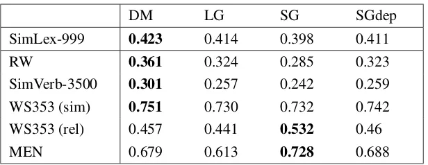
Table 1: Word similarity evaluation results, the values are Spearman’s correlation coefficients.
4.1 Word Similarity Datasets
Word similarity evaluation is one of the most common methods of testing vector space semantic models. The similarity datasets consist of word-pairs associated with human-assigned similarity scores. The task is to measure how well the model’s scores, obtained using the learned embeddings, correlate with the gold-standard. After the scores are computed for each pair, typically using the cosine similarity measure, the pairs are ranked by these values. This ranking is then compared to the gold-standard ranking using Spearman’s rank correlation coefficient.
The datasets used for this evaluation included Agirre et al. (2009)’s relatedness and similarity splits of WordSim353 (WS353) (Finkelstein et al., 2001), MEN (Bruni et al., 2014) which consists of 3000 similar and related pairs, the Rare Word (RW) collection (Luong et al., 2013), incorporating 2034 pairs of infrequent and morphologically complex words, SimLex-999 (Hill et al., 2016) consisting of 999 similar word pairs and SimVerb-3500 (Gerz et al., 2016) which includes 3500 similar verb-only pairs.
The models performed best using 300 dimensional embeddings and 20 negative samples (apart from SG, which performed best with 15 samples). As reported in Table 1, DM outperformed LG on all benchmarks and SGdep on allsimilaritydatasets. The latter demonstrates that the labels are a valuable information source and our model’s superiority over LG should not be attributed solely to decreasing data sparsity. Despite being trained on three times less training examples than SG, DM and SGdep managed to beat SG on all datasets but MEN and WS353 (rel). Importantly, both of these datasets measure relatedness rather than similarity.
4.2 RELPRON
RELPRON was introduced by Rimell et al. (2016) as an evaluation dataset for semantic composition. It consists of term-property pairs, with each term matched to up to ten properties. Each property takes the form of a hypernym of the term, modified by a simple relative clause. For example, the termdoghas the property mammal that people walk. The full dataset consists of 1087 properties and 138 terms, with a test set of 569 properties and 73 terms and a development set of 518 properties and 65 terms. The task is to determine matching properties for all terms. This is framed as an information retrieval task – for each term the properties are ranked according to their similarity to that term and the matching properties should have the highest ranks. The correctness of the rankings is assessed using Mean Average Precision (MAP). An alternative task is to determine the correct term for each property. Here, the evaluation measure becomes Mean Reciprocal Rank (MRR), as each property has only one matching term.
In RELPRON evaluation we sought to investigate the utility of the dependency context representa-tions for semantic composition. Since each property contains the term’s hypernym, it is easy to determine the relations between the term and the words in the property. For both MAP and MRR rankings, we con-structed a vector for each property, and then used cosine similarity between term vectors and property vectors. We experimented with two approaches to constructing property vectors, both based on weighted vector addition, which Rimell et al. (2016) showed to perform well as a composition method, despite its simplicity. The first, simple-sum (SS), is the sum of the words’ input-embeddings. The second,
DM LG SG SGdep
Development set
MAP (SS) 0.390 0.354 0.451 0.418
MAP (ES) 0.472 0.426 0.485 0.497
MRR (SS) 0.525 0.489 0.567 0.523
MRR (ES) 0.612 0.592 0.614 0.587
Test set
MAP (SS) 0.324 0.292 0.436 0.371
MAP (ES) 0.400 0.315 0.475 0.439
MRR (SS) 0.465 0.444 0.549 0.501
[image:7.595.144.449.69.254.2]MRR (ES) 0.557 0.509 0.574 0.543
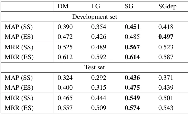
Table 2: Results of MAP and MRR evaluation on the test and development sets of RELPRON.
Simple-sum composition
Simple-sum composes a property representation by summing the input-embeddings of the agenta, verbv and patientpin a phrase4. The final similarity metric is the cosine between the resulting vector and the term’s input-embedding:
cos(Et, Ea+Ev+Ep)
Enhanced-sum composition
The motivation behind the enhanced-sum formula is to compose semantic representations of phrases based on a dependency graph, with a focus on one specific word – in this case, the head noun, which is the term’s hypernym.
There are two ways that we can view the head noun: as a target word, or as a context. Viewing the head noun as a target word, the verb acts as a context, and the other noun acts as afurther context. To represent the phrase, we therefore want to sum the head noun’s input embedding, the verb’s context embedding, and the other noun’s further context embedding. This composed vector should be close to the term’s input embedding.
Viewing the head noun as a context, the verb acts as the target word, and the other noun also acts as a context. To represent the phrase, we therefore want to sum the head noun’s context embedding, the verb’s input embedding, and the other noun’s context embedding. This composed vector should be close to the term’s context embedding.
Because of these two ways that we can view the head noun, in all of the following formulae, there are two cosines. The exact formulae differ across the models, as each model represents contexts differently. For the dependency models, the formulae also depend on the semantic role of the head noun (agent or patient), as it determines which dependency-matrices are used. Below, we present the formulae for the case where the hypernym is the agent, as in fuel: material that supplies energy. The case where the hypernym is the patient is analogous, but with different labels for the dependencies.
material (fuel) supplies energy.
nsubj
dobj
4We ignore the relative pronoun in the property representation as its contribution to semantics in RELPRON is indicating
For Skip-gram and SGdep, the dependency labels are not used. There is no way to represent a further context (a path of multiple dependencies) except as a normal context, so the enhanced-sum uses the following (noteOpfor the further contextp):
cos(Et, Ea+Ov+Op)
+cos(Ot, Oa+Ev+Op)
For LG, the context word and dependency are combined. There is no way to represent a further context. Unlike for Skip-gram, it would be problematic to use Op/dobj, because the head noun would never have been observed with adobjcontext during training. We instead use the input embeddingEp:
cos(Et, Ea+Ov/nsubj−1+Ep)
+cos(Ot/nsubj, Oa/nsubj+Ev+Op/dobj)
For DM, we have a principled way to represent the further context, through the multiplication of two dependency matrices. The input embedding Ep is mapped by TdobjT −1 to the output embedding space,
and then mapped byTnsubj−1 to the input embedding space.5 This composition method (multiplying
dependency matrices, and summing over words) can be applied to any possible dependency graph:
cos(Et, Ea+Tnsubj−1Ov+Tnsubj−1TdobjT −1Ep)
+cos(TnsubjOt, TnsubjOa+Ev+TdobjOp)
For RELPRON evaluation, DM and SGdep performed best using 300 dimensional embeddings and
m, the number of negative samples, set to 20. SG used 300 dimensions and m=15, while LG 200 dimensions and m=5. The results in Table 2 demonstrate that the DM model is once again superior to LG, outperforming the latter on both MAP and MRR evaluation. Overall, Skip-gram is the best performing model. As discussed by Emerson and Copestake (2017), models capturing relatedness can perform well on RELPRON, as they directly recognise the association between the term and the other argument of the verb (fuelandenergyfrom the previous example).
All models benefit from ES, which proves our proposed composition method is viable. Notably, the enriched similarity metric is particularly beneficial for DM, which experiences the highest performance increase: on the development set DM’s MAP (ES) and MRR (ES) scores are competitive to that of SG. This demonstrates the information encoded in DM’s dependency-enhanced contexts is valuable for this task and the proposed representations of further contexts work well. Training the model on longer dependency paths could further increase its performance, but we leave this for future work.
The general performance drop on the test set, also observed by Emerson and Copestake (2017) and Rimell et al. (2016), could be attributed to a number of factors, including the test set being∼10% larger than the development set and containing moregeneric properties, ranked highly by many terms. For example, in DM evaluation it contained 26 properties which appeared in the top 15 ranking of 7 or more terms (out of 73). In comparison, the development set had only 9 such properties.
4.3 Similarity vs Relatedness
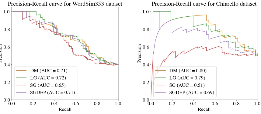
To test the model’s ability to distinguish between similarity andrelatedness relations we evaluated it on the task of ranking similar word-pairs above related ones. For this evaluation, following Levy and Goldberg (2014), we incorporated WS353 and Chiarello et al. (1990)’s dataset that Turney (2012) used for differentiating between functional and domain similarities. For both datasets we plotted precision-recall curves based on the rankings and calculated the AUC values. In the case of WS353, we disregarded the pairs that appear in both similarity and relatedness splits, which constituted the majority of pairs with scores equal or lower than 5 (out of 10). Figure 3 demonstrates that all dependency models are superior to SG on this task and there is not much difference in their performance.
5
More precisely, the model is trained to maximiseEp·Tdobj−1Ov, so we expectTdobjT −1Epto be close toOv. The model
is also trained to maximiseEa·Tnsubj−1Ov, so we expectTnsubj−1Ovto be close toEa. Combining these two results, we
Figure 3: Precision-recall curves showing the results on ranking similar pairs above the related ones.
DM LG SG SGdep
dolphin whale, shark, sailfish, porpoise
porpoise, giraffe, seahorse, orca
bottlenose, tursiops, stenella, delphis
whale, seahorse, shark, porpoise voldemort hordak, soth,
sidious, ganondorf
saruman, darkseid, hordak, melkor
dumbledore, horcrux, hagrid, dementors
melkor, xykon, hordak, ganondorf abba sizzla, tvxq,
mecano, cascada
roxette, a-ha, t.a.t.u., n.w.a.
agnetha, f¨altskog, lyngstad, eban
roxette, a-ha, n.w.a, tider cycling swimming, skiing,
speedskating, motorcycling
bicycling, biking, yachting, wakeboarding
bicycling, cyclo-cross, bicycle, biking
[image:9.595.72.528.305.420.2]biking, motorcycling, luge, snowboarding
Table 3: Examples of word similarities learned by the models.
4.4 Qualitative Evaluation
To inspect the types of similarities captured by the models we made a selection of four words from the vocabulary and analysed their closest neighbours according to each model. The examples presented in Table 3 confirm Levy and Goldberg (2014)’s findings, with SG capturing both similarity and related-ness and the dependency models demonstrating a bias towards similarity. Good examples of that are the neighbours of abbaor voldemort. For the first SG selected words such as agnethaor lyngstad – the names of members of the Swedish pop group ABBA. The dependency models, on the other hand, associatedabbawith other music bands, such as A-ha, Roxette or Sizzla. Forvoldemort, a villain from the Harry Potter series, the dependency models considered other fictional villains as most similar, while SG returned mostly names of characters from the books.
4.5 Dependency Parsing
In this experiment we used the input-embeddings of DM, LG and SG to initialise word representations of the Stanford Neural Network Dependency parser (Chen and Manning, 2014). The parser was trained and tested on the English Penn Treebank; sections 2–21 of WSJ were used for training, section 22 for development, while section 23 was reserved for testing. We trained the model for 20000 iterations using the default hyperparameters6. The embeddings were fine-tuned to the task during training. In addition to initialising the parser with input-embeddings, for the DM model using 50 dimensions we experimented with concatenations of the input and output-embeddings. We refer to this setting as DMio. Note that this could not be done for LG, as it only provides a single representation for each word.
DM and SG performed best with 100 dimensions, while LG used 50. Table 4 presents the results
6
DM LG SG DMio Dependency Parsing
UAS 91.49 91.40 91.33 92.01
LAS 90.02 89.99 89.82 90.66
POS Tagging (accuracy)
tuned 95.58 95.69 95.53 95.69
fixed 95.25 95.28 94.30 94.71
Chunking (accuracy)
tuned 92.66 93.11 92.68 92.84
[image:10.595.160.437.70.222.2]fixed 92.45 92.06 92.28 92.57
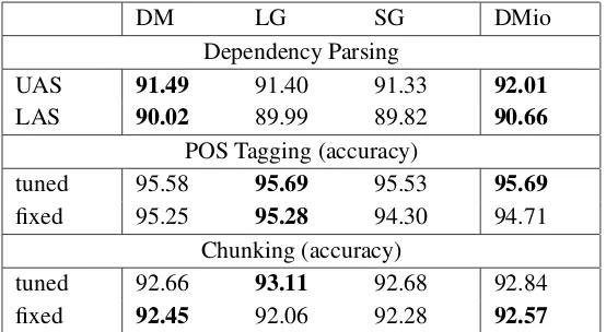
Table 4: Results of the dependency parsing, part-of-speech tagging and chunking evaluation.
achieved by the models measured with the unlabeled (UAS) and labeled attachment scores (LAS). Al-though all models performed well on this task, DM proved to be the best input-embedding initialisation. DMio performed overall best, demonstrating that utilising information encoded in the output-embeddings can be more beneficial than simply increasing the dimensionality of the embeddings.
4.6 Part-of-speech Tagging
For the POS tagging we made use of the publicly available word embedding evaluation framework,
VecEval(Nayak et al., 2016). VecEval’s word-labelling model resembles the one introduced by Collobert et al. (2011). First, it constructs the representation of the token’s context by concatenating embeddings of the surrounding words and then passes it through two neural network layers, followed by a softmax classifier. We trained and tested this model using the same WSJ splits used for the dependency parsing task. We initialised the model with the embeddings of DM, LG and SG and experimented with two settings: one that allows fine-tuning the embeddings to the task through backpropagation (tuned) and one that keeps the embeddings fixed (fixed). For POS tagging DM and SG performed best with the same embedding dimensions as for the dependency parsing, while best LG model used 100 dimensions. Table 4 demonstrates that in thetuned setting all models achieve comparable performance, while in thefixed
setting, both dependency models outperform SG, with LG reaching overall best performance.
4.7 Chunking
We evaluated SG, DM and LG on the chunking CoNLL’00 shared task (Tjong Kim Sang and Buchholz, 2000), which uses WSJ sections 15–18 for training and section 20 for testing. Similar to POS tagging, we employed theVecEval’s model based on that of Collobert et al. (2011) and experimented withfixed
andtuned settings. The best performing models followed the same hyperparameter setting as for POS tagging. The results presented in Table 4 show that in the tuned setting LG reaches the best perfor-mance, while in thefixed setting, which allows us to investigate information inherently present in the embeddings, DM outperforms the other models.
5
Conclusion
References
Agirre, E., E. Alfonseca, K. Hall, J. Kravalova, M. Pas, and A. Soroa (2009). A study on similarity and relatedness using distributional and WordNet-based approaches.Human Language Technologies: The 2009 Annual Conference of the North American Chapter of the ACL(June), 19–27.
Bansal, M., K. Gimpel, and K. Livescu (2014). Tailoring continuous word representations for depen-dency parsing. In Proceedings of the 52nd Annual Meeting of the Association for Computational Linguistics (Volume 2: Short Papers), pp. 809–815. Association for Computational Linguistics.
Baroni, M. and A. Lenci (2010). Distributional memory: A general framework for corpus-based seman-tics.Computational Linguistics 36(4), 673–721.
Baroni, M. and R. Zamparelli (2010). Nouns are vectors, adjectives are matrices: Representing adjective-noun constructions in semantic space. InProceedings of the 2010 Conference on Empirical Methods in Natural Language Processing, pp. 1183–1193. Association for Computational Linguistics.
Bengio, Y., R. Ducharme, P. Vincent, and C. Jauvin (2003). A neural probabilistic language model.
Journal of machine learning research 3(Feb), 1137–1155.
Bruni, E., N.-K. Tran, and M. Baroni (2014). Multimodal distributional semantics. Journal of Artificial Intelligence Research 49, 1–47.
Chen, D. and C. D. Manning (2014). A fast and accurate dependency parser using neural networks. InProceedings of the 2014 Con- ference on Empirical Methods in Natural Lan- guage Processing (EMNLP), pp. 740–750.
Chiarello, C., C. Burgess, L. Richards, and A. Pollock (1990). Semantic and associative priming in the cerebral hemispheres: Some words do, some words don’t... sometimes, some places. Brain and language 38(1), 75–104.
Collobert, R., J. Weston, L. Bottou, M. Karlen, K. Kavukcuoglu, and P. Kuksa (2011). Natural language processing (almost) from scratch. Journal of Machine Learning Research 12(Aug), 2493–2537.
Emerson, G. and A. Copestake (2017). Semantic composition via probabilistic model theory. In Pro-ceedings of the 12th International Conference on Computational Semantics (IWCS).
Finkelstein, L., E. Gabrilovich, Y. Matias, E. Rivlin, Z. Solan, G. Wolfman, and E. Ruppin (2001). Placing search in context: The concept revisited. InProceedings of the 10th international conference on World Wide Web, pp. 406–414. ACM.
Flickinger, D., S. Oepen, and G. Ytrestøl (2010). WikiWoods: Syntacto-semantic annotation for English Wikipedia.7th International Conference on Language Resources and Evaluation.
Gerz, D., I. Vuli´c, F. Hill, R. Reichart, and A. Korhonen (2016). SimVerb-3500: A large-scale evaluation set of verb similarity. InEMNLP.
Goldberg, Y. and O. Levy (2014). word2vec explained: Deriving Mikolov et al.’s negative-sampling word-embedding method.arXiv preprint arXiv:1402.3722.
Grefenstette, G. (1994). Explorations in Automatic Thesaurus Discovery. Norwell, MA, USA: Kluwer Academic Publishers.
Harris, Z. S. (1954). Distributional structure. Word 10(2-3), 146–162.
Levy, O. and Y. Goldberg (2014). Dependency-based word embeddings. In Proceedings of the 52nd Annual Meeting of the Association for Computational Linguistics, Volume 2, pp. 302–308.
Lin, D. (1998). Automatic retrieval and clustering of similar words. InProceedings of the 17th interna-tional conference on Computainterna-tional linguistics-Volume 2, pp. 768–774. Association for Computational Linguistics.
Luong, T., R. Socher, and C. D. Manning (2013). Better word representations with recursive neural networks for morphology. InCoNLL, pp. 104–113.
Melamud, O., D. McClosky, S. V. Patwardhan, and M. Bansal (2016). The role of context types and dimensionality in learning word embeddings. InHLT-NAACL.
Mikolov, T., K. Chen, G. Corrado, and J. Dean (2013). Efficient estimation of word representations in vector space. ICLR Workshop.
Mikolov, T., I. Sutskever, K. Chen, G. S. Corrado, and J. Dean (2013). Distributed representations of words and phrases and their compositionality. pp. 3111–3119.
Nayak, N., G. Angeli, and C. D. Manning (2016). Evaluating word embeddings using a representative suite of practical tasks. InProceedings of the 1st Workshop on Evaluating Vector-Space Representa-tions for NLP, pp. 19–23.
Nivre, J., M.-C. de Marneffe, F. Ginter, Y. Goldberg, J. Hajic, C. D. Manning, R. McDonald, S. Petrov, S. Pyysalo, N. Silveira, R. Tsarfaty, and D. Zeman (2016). Universal dependencies v1: A multilingual treebank collection. InProceedings of the Tenth International Conference on Language Resources and Evaluation (LREC 2016). European Language Resources Association (ELRA).
Pad´o, S. and M. Lapata (2007). Dependency-based construction of semantic space models. Computa-tional Linguistics 33(2), 161–199.
Paperno, D., N. The Pham, and M. Baroni (2014). A practical and linguistically-motivated approach to compositional distributional semantics. InProceedings of the 52nd Annual Meeting of the Association for Computational Linguistics, pp. 90–99. Association for Computational Linguistics.
Rimell, L., J. Maillard, T. Polajnar, and S. Clark (2016). RELPRON: A relative clause evaluation data set for compositional distributional semantics.Computational Linguistics 42(4), 661–701.
Sag, I. A. (1997). English relative clause constructions. Journal of linguistics 33(2), 431–483.
Schuster, S. and C. D. Manning (2016). Enhanced English universal dependencies: An improved repre-sentation for natural language understanding tasks.
Tjong Kim Sang, E. F. and S. Buchholz (2000). Introduction to the conll-2000 shared task: Chunking. In Proceedings of the 2Nd Workshop on Learning Language in Logic and the 4th Conference on Computational Natural Language Learning - Volume 7, ConLL ’00, pp. 127–132. Association for Computational Linguistics.
Turney, P. D. (2012). Domain and function: A dual-space model of semantic relations and compositions.