Modelling Multi operator Base Station Deployment Patterns in Cellular Networks

(1)

Modelling Multi-operator Base Station

Deployment Patterns in Cellular Networks

Jacek Kibiłda, Boris Galkin and Luiz A. DaSilva

F

Abstract—Stochastic models of base station infrastructure deployment by multiple mobile operators can be an invaluable tool for deriving fun-damental results about wireless network sharing. In this paper, we study stochastic geometry models for a shared cellular network consisting of base stations deployed by multiple mobile operators, based on real cellular network data coming from three European countries. Relying on a statistical approach as well as the evaluation of wireless network performance metrics, we find that, in the city center areas, operators tend to deploy their antennas in close proximity, while in other areas this is not the case and we find some level of repulsion between antennas of different operators. As we show, the log-Gaussian Cox process provides the most compelling fitness results with real multi-operator base station deployment patterns and a potentially attractive model that offers some degree of analytical tractability. Moreover, we observe that the behaviour which can be modelled with the help of these processes occurs over and over again for similar areas in different countries, which suggests universality of the proposed models.

Keywords—mobile networks, network sharing, infrastructure sharing, stochastic geometry, log-Gaussian Cox process.

J. Kibiłda, B. Galkin, and L. DaSilva are all with CONNECT, Trinity College, The University of Dublin, Ireland, email: {kibildj,galkinb,dasilval}@tcd.ie.

1 INTRODUCTION

Modelling and simulating the performance of shared wireless networks is of high importance to the research community and even more so to the cellular networks industry. From a technical perspective, sharing has been ongoing for a while now, predominantly in the form of sharing masts and antenna sites between mobile oper-ators, which is often referred to as passive sharing [1]. More recently, we have been witnessing an increase in active forms of sharing, which involve some level of resource virtualization that allows individual operators to jointly utilize base stations and/or the core network [2]. We see examples of this approach appearing more and more in response to the large costs associated with the provisioning of wireless cellular infrastructure. Some commercial examples of this type of sharing include the

merger of T-Mobile and Orange networks in Poland1, the

joint venture of two mobile operators in Denmark2 _or

the recent deal between Eircom and Three in Ireland3_.

The fundamental gains and limitations of such shared networks are still an open question, and the research to date has been rather conservative in treating the topic. To quantify these gains and limitations, there is the need for accurate models that are representative of the super-position of radio access network deployments made by multiple mobile operators. Herein, we make a contribu-tion to the state-of-the-art in wireless network modelling by providing a quantitative analysis of stochastic models that may be used to represent shared cellular network deployments.

In general, wireless network deployment can be mod-elled as a collection of points distributed on a two-dimensional plane. Each point, representing a base sta-tion (BS) transceiver, is assigned some wireless network related properties, such as downlink transmit power and operational frequency. Then, the average performance experienced by a user of such a network may be obtained either using stochastic geometry or through computer simulations. In stochastic geometry a typical working as-sumption is to use a homogeneous Poisson point process

1. The process is comprehensively described in the following slides: http://www.slideshare.net/zahidtg/deployment-of-ran-sharing-in-poland (accessed 22.10.2014).

2. http://www.fiercewireless.com/europe/story/teliasonera-and-telenor-given-ok-network-sharing-jv/2012-03-02

(2)

(PPP) to represent network deployment. While in com-puter simulations the hexagonal lattice model is used. These models may serve as a reasonable representation of single-operator networks, see [3]. However, when as-sessing a real BS infrastructure deployment coming from

multiple operators, we see significant degree of clustering across operators, related, most likely, to the competition for demand that is unevenly distributed across space, see [4]. The above models are insufficient to capture this type of behaviour, and thus our goal is to identify more appropriate models that capture the key properties of

multi-networks(networks that combine deployments from multiple operators), which requires application of tools from spatial statistics.

An elementary step in any spatial statistics analysis is the qualitative assessment, which builds rationale for further modelling decisions. Fig. 1 depicts four patterns representing two-operator BS deployments using: a su-perposition of two realizations of the hexagonal lattice model (Fig. 1a), a superposition of two realizations of the Poisson point process (Fig. 1b), a realization of a clustered point process (Fig. 1c), with operator marks assigned uniformly at random, and a real BS deployment in the Dublin city area (Fig. 1d). Clearly, we can observe a high degree of regularity with the hexagonal deployment and uniformity with the PPP deployment. The clustered deployment results in a number of smaller clusters dis-tributed throughout the area of interest and relatively many empty spaces, in comparison to the previous two realizations. Finally, the pattern representing real deploy-ment is clustered around the central area with blank areas forced by environmental obstacles, and somewhat uniform or repulsive behaviour outside the central area, possibly caused by frequency and coverage planning as well as low availability of shared BS sites. Qualitatively, one can conclude that the first two point patterns and the real one come from distinct families of point distri-butions. The relationship between the clustered pattern and the empirical pattern is less intuitive, and, as we will show later, the realizations of some of the clustered point processes do indeed convey the features of multi-operator real BS deployments.

In order to support our claims, we delve into statistical data analysis and wireless network performance evalua-tion, relying on real BS deployments in three countries. In this paper, we report our model fitting results for various point processes in various locations, indicating the models that best describe our data, and discuss the potential usability of the models for shared wireless network analysis.

Main contribution In this paper, we identify point processes that model a cellular network consisting of base stations belonging to multiple operators (a multi-network), operating in urban environments. We base our work on BS deployment data coming from Ire-land, Poland and the UK. What we observe is that multi-networks cannot be simply modelled with a su-perposition of independent realizations of a point

pro-cess describing a operator deployment (a single-network). In fact, as we show later, there is a high degree of dependence between the infrastructure deployment made by multiple operators. This quantitative result supports intuition which suggests that commercial net-works are designed and deployed to satisfy the demand unevenly spread across geographic areas by competing operators offering similar services.

In order to find the model that best fits multi-networks, we apply a spatial statistics approach [6]. Namely, we calculate the empirical estimates of the pair-correlation function, which is a second-order characteristic, and we fit the point processes to those estimates using the meth-ods of maximum pseudolikelihood, whenever possible, and minimum contrast [7]. Subsequently, we evaluate goodness-of-fit of our estimated models by comparing empirical estimates of some other summary statistics obtained from the real data against maximum and min-imum values of the same statistics calculated for our estimated models. In the course of our analysis we find that the clustered point processes best represent base station clustering occurring in multi-networks, with the log-Gaussian Cox process (LGCP) providing the most compelling fitness results and a potentially attractive op-tion for some degree of analytical tractability. Moreover, we observe that this clustering behaviour, which can be modelled with the help of clustered point processes, occurs over and over again for similar areas in different countries, which indicates some degree of universality of the proposed models.

2 RELATED WORK

(3)

[image:3.612.69.556.56.192.2]

(a) Hexagonal (b) Poisson (c) log-Gaussian Cox (d) Real

Fig. 1: Illustration of different types of two-operator BS deployment patterns for the city of Dublin (the Dublin city area is represented here as a superposition of the smallest unit areas provided in [5], and located within a radius of 5 km from the city’s center), generated from: a) a hexagonal lattice, b) a Poisson point process, c) a clustered point process, and d) real data. The contours represent the Dublin city area, whereas the dots and triangles stand for BS site locations of two different operators. The real BS pattern is clustered in the central area, with irregular empty spaces forced by environmental obstacles and, most likely, coverage planning. Qualitatively, the clustered point process realization exhibits the closest match to the real BS pattern, with a number of smaller clusters distributed throughout the area of interest and relatively many empty spaces, while the Poisson point process pattern rather uniformly fills the Dublin area and the hexagonal pattern exhibits high regularity with little resemblance to the actual BS deployment.

Moreover, the incumbent mobile network operators, as a natural cost minimization strategy, will tend to reuse existing sites [8]. Effectively, even initial coverage pro-visioning deployment may be allocated in a way that is far from idealistic lattice-like scenarios. Furthermore, as the service demand grows, and large capacities be-come essential, a microcellular topology is deployed, typically characterized by much lower transmit powers and rooftop level antennas, with additional pico-/small-cell systems to extend the capacity to indoor offices or places like shopping malls.

Despite these practical insights on the cellular network roll-out process, there seems to be no consensus on how to model and analyse the resulting BS deployments. In the studies to date the choice of a model is typically dependent on the type of tool applied, either stochastic geometry or computer simulation.

Stochastic geometry allows us to derive analytical expressions for various performance parameters, such as outage probability or data rate, under predefined wireless channel conditions, averaged over many realiza-tions of a pre-specified stochastic model. For analytical tractability, much of the existing work modelling radio access network deployments (e.g., [11], [12], [13], [14]) relies on the homogeneous PPP model, which assumes no correlation in the analysed patterns. The usage of the PPP model can be analytically justified under suf-ficiently high log-normal shadowing, see [15]. However, spatial statistical analysis of the available mobile network deployment data to date suggests that single-operator mobile networks can be better represented using

reg-ular processes. For example, in [3] the fitted Strauss process turns out to provide the closest match to a single-operator mobile network deployment. In [16] the determinantal point process (DPP) is found to accu-rately represent regularities present in single-operator base station deployments. Analytical insights into these point processes are limited to some specific cases, see [17]. Yet, heuristic approaches, such as the one in [18], may be applied. Clustering in real mobile networks, as observed in large-scale single-operator deployments [19], can be modelled using cluster processes. However, analysis of these processes seems to be even harder and some level of analytical tractability has been achieved only for certain classes of cluster processes, see [20].

(4)

[3], [16]). It is worth mentioning that simulations based on a hexagonal lattice model predominate in the research to date which attempts to evaluate the performance of wireless network sharing, see [22], [23], [24], [25].

In our work we seek point process models that are representative of the base station infrastructure deploy-ments by multiple operators. We evaluate these models by fitting them to real infrastructure data coming from three different countries and performing a series of fit-ness tests, which give us statistical confirmation of the correctness of the selected model(s).

3 B

ACKGROUND AND NOTATION

A wireless network deployment can be represented as a point process which is a countable random collection of points that lie in the Euclidean plane [26]. Herein, we describe such a point process as a random countable

set Φ = {x1, x2, ...} ⊂ R2 with elements being random

variables xi ∈ R2. Using the random counting measure

formalism [26], we also denote ϕ as a realization of Φ,

and ϕ(W)as the number of points in the realization ϕ

distributed over a finite observation window W ⊂ R2.

Moreover, we denote Λ(W) as the intensity measure of

Φ, which, informally, is the mean number of points of a

point process Φ in a set W. In consequence, λ(x) will

denote the intensity function that describes the point

density around location x∈R2_.

There are three general classes of point processes: uni-form, clustered and regular. To say that a point process is uniform is equivalent to assuming that no inter-point interactions can be observed in a point pattern coming from that process. Clustering means that some form of positive interaction (attraction) exists between points, leading to clustered patterns, while regularity stands for some form of negative interaction (repulsion) be-tween points in the process. Since multi-network patterns exhibit, at least qualitatively, some form of clustering we focus our attention on point processes that allow us to model this phenomenon. Namely, in our work we rely on three point processes: the log-Gaussian Cox process (LGCP), the Matern cluster process (MCP), and the Thomas process (TP). However, in order to get the full picture of the kinds of interactions one may expect in such BS deployments we also test whether the observed point patterns follow either the homogeneous PPP or possibly a superposition of a number of independent realizations of the Strauss process (SP), which was shown to provide a good fit to single-networks [3]. While Guo and Haenggi in [3] have already introduced the PPP and the SP, in the following we briefly introduce the Cox processes and the cluster processes. More comprehensive description of all these point processes can be found in [6], [7], [26].

3.1 Cox processes

Cox processes describe spatial point patterns which ex-hibit some forms of aggregation or clustering, typically

caused by some random environmental phenomenon [7]. The Cox process is obtained as a generalization of the inhomogeneous PPP, where the intensity measure of the point process becomes random. Conversely, conditioned on the intensity measure the resulting point process is Poisson, and thus the Cox process is also referred to as thedoubly stochastic Poisson process.

Log-Gaussian Cox process We focus on a subclass of Cox processes, where the logarithm of the intensity function is a Gaussian process [27]. This subclass is called the log-Gaussian Cox process (LGCP), with the

intensity function denoted as λ(x) = exp (Y(x)), where

Y = {Y(x) : x∈ R2} is a real-valued Gaussian process

with mean µ, and covariance function σ2_f₍_r₎_{, where}

σ2 is the variance and f(r) is some pre-defined spatial

correlation function. For the LGCP to be well-defined the spatial correlation function has to be positive semi-definite [28]. This condition is met by, for example, the

exponential function f(r) = exp(−r/β) and the stable

function f(r) = exp(−p

r/β), where β > 0 is a scale

parameter (other examples of functions that meet this condition can be found in [28]). The LGCP is fully

characterized by µ, σ2 _{and the parameter(s) of} _f₍_r₎_,

which are easy to estimate due to the existence of closed-form expressions for the summary statistics. The process is also relatively easy to simulate based on the location dependent rejection of points generated according to the

homogeneous PPP with λ∗ = max(λ(x)). Moreover, the

intensity of the process is expressed asλ= exp(µ+σ2/2).

3.2 Cluster processes

Generally, cluster processes can be viewed as realizations of two hierarchical point processes: the parent point process, which distributes clusters, and the daughter point process, which distributes points around the parent point location. Typically the parent process does not lead to the generation of points, therefore the cluster process consists of the union of all daughter points.

Matern cluster process The Matern cluster process is a doubly Poisson cluster process, i.e., parent points are generated according to a Poisson process with intensity

κ, and daughter points, with the mean number of them

µ, are uniformly distributed inside the circle of radius

R centered at each parent point. The intensity of the

daughter process takes the following form:

λd(r) =

µ

v(b(o, R))1[b(o,R)](r), (1)

where1[b(o,R)](r)is an indicator function,b(o, R)denotes

a circle centered at parent point o with radius R, and

v(·) is the Lebesgue measure, which in the Euclidean

space corresponds to the surface area. The intensity of

the process is λ=κµ.

(5)

with intensityκ, while the daughter points are normally distributed, i.e., according to the intensity function:

λd(r) =

µ

2πσexp(−

r2

2σ2), (2)

whereµis the mean number of daughter points andσ2_is

the variance. The intensity of the process is againλ=κµ.

3.3 Summary characteristics

In spatial statistics there are numerous summary char-acteristics that describe and quantify local groupings of points, typically through their relative positions or inter-point distances. In the following we briefly introduce the metrics that we will subsequently use for model fitting and goodness-of-fit tests.

Generally, a point process that drives multi-network patterns is unknown. Therefore, to obtain each of the fol-lowing metrics we are required to utilize non-parametric estimators with appropriate methods to mitigate finite observation window distortions that occur at the edges. Moreover, since each of the analysed deployments has some local inhomogeneities, we normalize each charac-teristic obtained against inhomogeneities of the corre-sponding deployment.

Empty space function Empty space function F(r)

de-scribes the distribution of distancerfrom a pointo∈W

(for stationary point processes this corresponds to the

origin) to the nearest point of the point process Φ:

F(r) =P(||o−Φ|| ≤r) =P(ϕ(b(o, r))>0), r≥0. (3) We use the empty space function as the first-order goodness-of-fit statistic.

J-function One way to investigate the interaction be-tween two point patterns, each with a different type of points, observed within the same window, is to utilize the cross-type J-function [29]. The cross-type J-function is the ratio between the distributions of the distances from

an arbitrary fixed point of type i to the nearest type j

point, therefore it can be used to quantify clustering or repulsion between two sets of points. The cross-type J-function is given as:

Jij(r) =

1−Gij(r)

1−Fj(r)

, (4)

where Gij(r)is the nearest neighbour distance function,

which describes the distribution of distances from the

points of typej to the points of typei, and Fj(r)is the

empty space function of the point pattern of type j. In

case the two analysed point patterns are independent

Jij= 1, as is the case with any homogeneous PPP

realiza-tions. Jij <1 suggests that the points of different types

aggregate, while Jij > 1 suggests repulsion. However,

the cross-type J-function taking value 1 for allris not a

sufficient characterization of independence between the

two patterns [29]. It is also worth noting that Jij is not

symmetric in iand j.

L-functionThe L-function is defined asL(r) =pK(r)/π

for r ≥ 0, where K(r) is a second-order summary

characteristic which describes the mean number of points

within radius r from points in point process Φ. The

L-function is particularly useful in the estimation of model parameters, such as the interaction distance (maximum inter-point distance at which interaction force is at work) or interaction force (the force that describes mutual at-traction or repulsion between points in a point process). For the PPP the L-function takes a convenient linear

form L(r) = r. Hence, for some pattern ϕ, L(r) < r

will indicate regularity, while L(r) > r will indicate

clustering. We use the L-function to examine fitness of the estimated models with respect to second-order characteristics.

Pair-correlation function The pair-correlation function

g(r)for a stationary point processΦwith intensity

func-tion λand second order product density ρ(2)₍_r₎_{, which}

is the joint probability that there are two points of Φ

in infinitesimally small areas surrounding two locations

separated by distance r, is defined as follows [26]:

g(r) =ρ

(2)₍_r₎

λ2 . (5)

Informally, the pair-correlation function characterizes the frequency of inter-point distances in the process. Herein, we use the pair-correlation function for fitting clustered point processes to our data. The fitting method we use requires an analytical expression for the summary statis-tic in question. The expressions for the pair-correlation function of the analysed clustered point processes are summarized in Tab. 1.

4 DATASETS AND MODEL FITTING

4.1 Datasets

The aim of our study is to find a stochastic model that characterizes multi-networks aggregated for the purpose of infrastructure sharing. The input data we use consists of either real BS information or radio license information (for simplicity, we will assume that an assigned radio license is equivalent to a BS deployed in the given location), which includes spatial coordinates of the BS sites and unique cell identifiers, for GSM and UMTS technologies in three countries: Ireland, Poland, and the United Kingdom. The data was extracted from publicly available information collected by the national telecom-munications regulators. Each of the regulators collects data supplied by the local mobile network operators (MNO), who also ensure accuracy and keep the infor-mation updated.

The Irish database contains BS site information up-dated by the Irish MNOs and maintained by the Irish

communications regulator ComReg4_{. Based on the}

quar-terly report from ComReg (Q4 2013), Ireland had four

(6)

TABLE 1: Analytical expressions for the pair-correlation function of the analysed clustered models, where h(z) = 16/π(zarccos(z)−z2√₁₋_z2₎_for_z_≤₁ _and_h₍_z_{) = 0} _otherwise.

Model LGCP MCP TP

g(r) exp σ2_f₍_r₎ _{1 + (4}_πRrκ₎−1_h₍r

2R) 1 + (4πκσ

2₎−1_exp(₋r2

4σ2)

major MNOs (Vodafone, eircom Group Mobile, O2 and Three) together sharing 93.9% of the Irish mobile mar-ket. We deem the Irish dataset as the most reliable, as ComReg requires mobile infrastructure providers to report all the masts and structures that contain “mobile base stations”. Therefore, we use the Irish dataset to confirm the reliability of the other two datasets. The database for Poland contains spatially allocated radio license information from all MNOs operating in the Polish mobile market, available through the national

regulator UKE5_{. By 2013 there were four major MNOs in}

Poland, namely Orange, Play, Plus and T-Mobile, which had a combined 98.7% of the subscriber share and 99.7% of the market revenues. The database for the UK was compiled by OfCom (UK’s Office for Communications) based on BS site information voluntarily supplied by

the local MNOs6_{. As of 2012 there were five major local}

MNOs: O2, Orange, T-Mobile, Three, and Vodafone, all of them together having a higher than 90% market share. From each of the databases we have selected a number of city areas. For each city area we have focused on BS site information for two radio technologies: GSM (900 MHz) and UMTS (2100 MHz), and macro- and microcells only (if the transmit power or cell radius information was available). For each city area we have extracted this information for an observation window of size 10-by-10

km with arbitrarily selected central locations7_{. The choice}

of the observation window was driven by our desire to capture features of BS deployments at local scales, and to correctly assess environmental forces that underlay point distributions for multi-network deployments. In our study, we have simplified each co-location to a single BS site, which is a reasonable working assumption given that inter-operator co-location accounts on average for only 10% of all base stations. Tab. 2 summarizes basic information on all the selected locations.

Since the analysis covers different geographical areas as well as various statistical metrics, for clarity we have decided to focus our presentation on the study of Dublin. The results for other areas (listed in Tab. 2) are substan-tially the same and they are included in the estimated point process model, which we discuss at the end of this section.

5. http://www.uke.gov.pl/pozwolenia-radiowe-dla-stacji-gsm-umts-lte -oraz-cdma-4145

6. http://stakeholders.ofcom.org.uk/sitefinder/sitefinder-dataset/ 7. In order to test whether our results are affected by the choice of the observation window we also looked at observation windows of size 2.5-by-2.5 km, and 5-by-5 km. In the main, the results are consistent across those three observation windows.

4.2 Fitting method

A desirable model is one that is easy to interpret, esti-mate and simulate, while still preserving features of the observed BS patterns. Herein, we provide the results of fitting PPP, SP, MCP, TP and LGCP, with exponential and stable correlation functions, to the multi-network patterns under study. To fit the first two we have used the maximum pseudolikelihood method, described in [3]. When the pseudolikelihood function is not easily tractable, which is typically the case with clustered point processes, we apply the minimum contrast method (MCM) [7]. In general, the MCM seeks parameter values

for the analytical expression of a summary statistic C

which minimize the difference between C and its

non-parametric estimate obtained from the analysed patterns

ˆ

C, i.e.:

Dθ=

Z rmax

rmin

|Cˆ(r)q−Cθ(r)q|pdr (6)

where Cθ is the theoretical expression for the summary

characteristic parameterized with θ, while p and q are

simulation parameters. Applying the MCM to the anal-ysed processes is natural, as for each of those processes

we can obtain closed-form expressions for then-th order

summary characteristics. Specifically, we use the pair-correlation function, for which closed-form expressions

are given in Tab. 1. Settingp= 2, andq= 1(for the MCP

and TP), allows us to obtain closed-form expressions for the parameters of the fitted processes, which we summarize in Tab. 3. We derive these expressions in Appendix A.

In our analysis we look at a range of r values, where

rmin = mini6=j;xi,xj∈ϕ{||xi−xj||} (as suggested in [28])

and rmax is set as the quarter of the side-length of the

square observation window, which, according to our sim-ulations, provides a good balance between observation of the local features and computational effectiveness. We perform our analysis using open-source statistical computing software R [30], and, in particular, we use

functions from thespatstatlibrary [31]. For the

goodness-of-fit tests we use the envelope test, which can be in-terpreted as the significance test [6], with a significance

level in a one-sided test equal to1/(k+ 1), wherekis the

(7)

[image:7.612.127.493.79.208.2]

TABLE 2: Basic information on the extracted point patterns

Dataset Name Center (longitude;latitude)

Number of extracted BSs (UMTS/GSM)

Inter-operator co-location (UMTS/GSM) [%] Ireland Dublin 53.3478◦N;6.2597◦W 447/409 5.0/4.0 Poland

Kraków 50.0614◦N;19.9383◦E 348/273 8.0/8.0 Pozna ´n 52.4◦N;16.9167◦E 400/362 10.0/14.0 Warszawa 52.2333◦N;21.0167◦E 812/916 12.0/8.0

UK

Birmingham 52.4831◦N;1.8936◦W 281/144 5.0/0.0 Leeds 53.7997◦_N;₁_.₅₄₉₂◦_W _238/115 _16.0/0.0

Liverpool 53.4◦_N;₃◦_W _266/122 _7.0/0.0

[image:7.612.160.461.244.322.2]

London 51.5072◦N;0.1275◦W 1442/1513 3.0/1.0 Manchester 53.4667◦N;2.2333◦W 303/155 7.0/0.0

TABLE 3: MCM expressions for model parameters

Model Model parameters

I II III

LGCP µˆ= log(ˆλ)−σˆ2_/₂ _σ_ˆ2₌BL(β)

AL(β)

1/q _ˆ

β= argmax

BL(β)2

AL(β)

MCP µˆ=λˆ ˆ

κ Rˆ= argmax

BM(R)2

AM(R)

ˆ

κ=AM(R)

BM(R)

TP µˆ=λˆ ˆ

κ σˆ

2_{= argmax}

BT(σ2 )2

AT(σ2 )

ˆ

κ= AT(σ2 )

BT(σ2 )

4.3 Fitness results - Dublin case

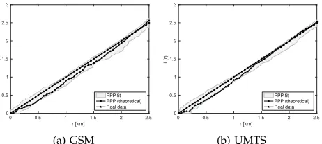
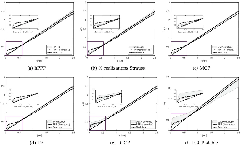
Before we turn to the multi-network analysis, we in-vestigate the L-function results for single-networks to confirm observations made in [3]. In Fig. 2 we ob-serve the L-function results for selected GSM and UMTS deployments, along with 99 realizations of a Poisson fit (corresponding to a significance level of 0.01), and its well-known closed-form representation. The results somewhat confirm the observations made in [3], as the observed point patterns for various operators in different areas exhibit either some mild forms of inhibition or uniformity for the whole range of inter-point distances.

We now turn our attention to the relationship be-tween multi-operator deployments. If single-networks

r [km]

0 0.5 1 1.5 2 2.5

L(r)

0 0.5 1 1.5 2 2.5 3

PPP fit PPP (theoretical) Real data

(a) GSM

r [km]

0 0.5 1 1.5 2 2.5

L(r)

0 0.5 1 1.5 2 2.5 3

PPP fit PPP (theoretical) Real data

(b) UMTS

Fig. 2: The L-function results for Meteor GSM and UMTS deployments in Dublin (marked with triangles) with the envelope of the fitted Poisson model at a significance level of 0.01 (grey area), and the theoretical value for the Poisson process (marked with circles).

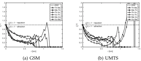
were realizations of independent Poisson processes, we would expect that the observed multi-network patterns should not exhibit any forms of regularity. However, as noted previously the resulting multi-network point patterns clearly exhibit clustering. This fact and the single-operator fit would suggest that the realizations of networks of different operators are not independent from each other, which also makes sense intuitively, as one would expect that BS placements account for local phenomena, such as high availability of potential subscribers. In order to test this hypothesis, we look into the cross-type J-function results for multiple opera-tors in Dublin. Since the J-function involves comparison between different patterns, we drop for a moment the assumption of simplicity and allow for BSs of different operators to co-locate. Both the results for GSM (Fig. 3a) and UMTS (Fig. 3b) confirm that there is significant clus-tering for the majority of inter-point distances, with some repulsive behaviour for Three-Meteor/Meteor-Three and Vodafone-Meteor pairs at larger distances, which may reflect the structure of the Irish mobile market and its existing infrastructure sharing among operators. Note that these results, as any results in empirical statistics, are merely an indication of clustering among the observed BS patterns rather than a formal proof.

[image:7.612.62.293.518.622.2]

(8)

r [km]

0 0.5 1 1.5

Jij

(r)

0 0.2 0.4 0.6 0.8 1 1.2 1.4 1.6 1.8 2

PPP Th-Me Me-Th Th-Vo Vo-Th Me-Vo Vo-Me

Jij(r) < 1 ~ attraction

Jij(r) > 1 ~ repulsion

(a) GSM

r [km]

0 0.5 1 1.5

Jij

(r)

0 0.2 0.4 0.6 0.8 1 1.2 1.4 1.6 1.8 2

PPP Th-Me Me-Th Th-Vo Vo-Th Me-Vo Vo-Me

Jij(r) < 1 ~ attraction

Jij(r) > 1 ~ repulsion

[image:8.612.54.299.50.157.2]

(b) UMTS

Fig. 3: The cross-type J-function results for combinations of pairs of major MNOs in Dublin: Meteor (Me), Three

(Th) and Vodafone (Vo). Recall that by definition Jij

is not symmetric and also Jij < 1 indicates clustering

(while Jij > 1 inhibition) between the BS locations of

any two MNOs.

r [km]

0 0.5 1 1.5 2 2.5

G(r)

0.5 1 1.5 2 2.5 3

PPP ub PPP lb Dublin Krakow Liverpool London Manchester Poznan Warszawa

(a) GSM

r [km]

0 0.5 1 1.5 2 2.5

G(r)

0.5 1 1.5 2 2.5 3

PPP ub PPP lb Dublin Krakow Liverpool London Manchester Poznan Warszawa

(b) UMTS

Fig. 4: The pair-correlation function for real deployments in various cities; Dublin marked with triangles and the envelope of the fitted Poisson model (at a significance level of 0.01) marked with solid lines.

significant clustering that occurs at inter-point distances below approximately 500 meters, beyond which point the patterns become somewhat uniform, with spikes of regularity or clustering occurring as a result of some unobserved local heterogeneities, most likely related to social and geographical features of the analysed areas. This result indicates that multi-networks in urban areas show similar behaviour, which gives us some confidence in the reliability of our input datasets and suggests that a single model could be potentially representative to a class of real multi-networks.

From Fig. 4 it is quite clear that any point process capa-ble of modelling multi-networks would need to exhibit short-range clustering and be robust enough to account for some deviations in local clustering and repulsion of points at larger distances. The model that intuitively is the most promising is the log-Gaussian Cox process, which allows us to parameterize and estimate the un-observed local covariates in the form of a random field spanning the analysed area. Since our goal is to find a point process that represents features of multi-networks, we look also at other clustered point processes, namely the Matern cluster process and the Thomas process. In order to show that multi-network patterns have strong

clustering features, which cannot be captured by pro-cesses describing single-networks, we also provide fitting results for other point processes: the PPP (to disprove the complete spatial randomness hypothesis [6]), and the superposition of independent SP realizations. The figures also include envelopes, which represent the maximum and minimum of 99 realizations of the fitted model, which are used to assess the goodness-of-fit of the model in the envelope test [6].

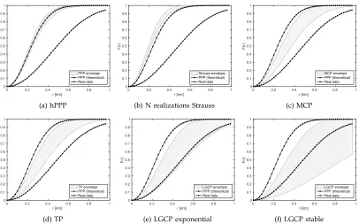
[image:8.612.53.299.245.349.2]

As we can see from Fig. 5 and Fig. 6 both the PPP and the superposition of independent realizations of the SP can be rejected as candidate models, since they do not produce sufficiently large empty spaces, both in the GSM and UMTS case. Moreover, these point processes are unable to model short-range clustering as can be seen from the results obtained for the L-function in Fig. 7 and Fig. 8. Doubly Poisson clustered models (MCP and TP), seen in Fig. 5 and Fig. 6, do not pass the envelope test for the F-function, as they under-represent the occurrence of empty spaces in the patterns. Moreover, when second-order characteristics are taken into account, these point processes seem to insufficiently capture clustering, while completely missing out on the long-range repulsion, see Fig. 7 and Fig. 8.

By far the most satisfying results we have observed come from the LGCP models, which in the UMTS case passed the F-function envelope test for both models, see Fig. 6, and for the GSM case passed the F-function test for the model with the stable correlation function, see Fig. 5. Apparently, the trade-off for achieving better fitness is related to increased variance in the occurrence of empty spaces prevalent in the modelled patterns. When it comes to second order statistics, we can see in Fig. 7 and Fig. 8 that both the LGCP models are able to account for the short-range clustering, while also being able to capture long-range repulsion in the patterns. In our simulations we have also tried other than the exponential and stable spatial correlation functions (for example, Gauss or spherical); however, fitting against a model based on either of the two functions gave us the most satisfying results.

4.4 Fitness results - other areas

(9)

cases, we have looked also at some areas with lower density of base stations, such as Athlone, Ireland. In order to obtain meaningful results for rural areas we had to increase the observation window size to 25-by-25 km. However, even increasing the observation win-dow left us with relatively small patterns that contained significant amount of empty spaces. In those patterns we could still observe some mild forms of clustering at smaller distances, which in most cases was enough to reject the PPP hypothesis. The considered clustered point processes were able to capture this clustering as well as the following uniformity in the pattern, although the fitted models had significant variance. And since these results were not entirely consistent across the other rural areas we have analysed, we have decided to focus on modelling urban locations.

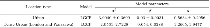
Based on the fitness results we have concluded that the most promising point process to model multi-networks in urban areas is the LGCP. Furthermore, we have observed that we can almost unambiguously classify the parameters of the models according to the type of deployment, i.e., urban, and dense urban. Tab. 4 sum-marizes the two classes of models we have found. It is interesting that for the urban scenario the standard deviation is relatively low (around 10%) for both shape

parameters, i.e., σ2 _and_β_{, which suggests similar shape}

of the intensity function λ(x)for each of the geographic

areas considered, with only scale parameter µ(precisely

exp(µ)) having higher deviation to account for the

dif-ferent number of BSs in each area. For the two dense urban areas (London and Warsaw) the estimated model parameters differ significantly, which is presumably the result of much higher number of base stations and much richer structure of the area (higher concentration of BSs, larger number of neighbourhoods with concentration of BSs).

5 PERFORMANCE ANALYSIS

Having evaluated the statistical match between our proposed point process models and real multi-network deployments, we now turn our attention to wireless network-relevant evaluation based on the radio access network sharing scenarios of: infrastructure, spectrum and full network sharing, as studied in [14]. As a metric

for our evaluation we use the coverage probability [26],

i.e., the complementary cumulative distribution function (CCDF) of SINR, which we obtain for each estimated deployment model and each scenario via Monte Carlo simulations.

In the following we assume that the power of the signal received by a typical user located in the origin

(0,0) is affected by two factors: pathlossl(x)and power

fading hx, where x denotes the location of the serving

BS. The pathloss function l : R2 _→ _R

+ is of the form

l(x) = ||x||−α_{, where} _α _{is the pathloss exponent, and}

the power fading between the user and the serving

transmitterxis spatially independent and exponentially

distributed (e.g., Rayleigh fading) with mean µx which

corresponds to the transmit power of a BS located in

x, i.e., hx ∼ exp(1/µx). In the following we analyse

two approaches to assigning transmit powers to BS

transmitters: initially, we set µx = 1 for all x ∈Φ, and,

subsequently, we extend our model and assign transmit powers according to the scheme we proposed in [32]. In addition, we make the following assumptions: (i) our results apply to the downlink only, (ii) worst-case interference is considered, i.e., all transmitters transmit simultaneously, (iii) we assign individual BSs to oper-ators uniformly at random, (iv) noise is unitary for all

the receivers, and (v) α = 4. For each realization of

the estimated model we generate 2000 user locations, over which we average our results. We also apply edge-effect correction based on an enlarged window, i.e., we assume that the user locations lie inside a square window centered at the analysed area with the side equal to half the side of the window containing the original area.

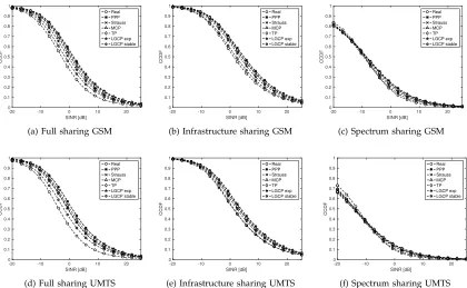
Coverage probability - unitary transmit power

Fig. 9 presents the coverage performance of our mod-els for each of our sharing scenarios and technologies when BS transmit power is unitary. In each case the LGCP model with the stable correlation function gets the closest to the coverage provided by a real multi-operator network. In the case of full network sharing our models significantly over-estimate the amount of coverage in the network (approx. 2 dB vertical shift for the “LGCP stable” model). However, in the case of infrastructure sharing we observe that the “LGCP stable” model provides a very tight match to a shared network performance. The spectrum sharing scenario provides significantly worse coverage, which should come as no surprise as we assumed worst-case interference. Interest-ingly, in the case of spectrum sharing we observe a cross-over point, which we have reported also in [14], which is related to the amount of clustering in the evaluated patterns. Clearly, a real multi-network provides higher clustering than any of our models can produce. It is also worth noting that, while statistical tests have shown that a superposition of independent realizations of the Strauss process provide a reasonably good match to the real data, according to our coverage analysis this way of modelling multi-operator patterns fails to reproduce cov-erage properties of multi-networks in wireless network sharing scenarios.

Coverage probability - transmit power assigned as proposed in [32]

(10)

[image:10.612.129.493.79.129.2]

TABLE 4: Fitted model parameters

Location type Model Model parameters

σ2 β µ

Urban LGCP 3.9040±0.3699 0.03±0.0031 −0.5634±0.2956

Dense Urban (London and Warszawa) LGCP 2.0561,2.7228 0.054,0.0288 1.2665,1.9477

transmit powers.

The first thing we observe in Fig. 10 is that BS transmit power assigned from a model based on real data has a negligible impact on the coverage of the analysed network model (the coverage probability is degraded by roughly 1% for each SINR point), which is consistent with our prior observations [32]. This is true also when the noise level of -130 to -90 dBW is included at the receiver. This result is good news as it allows us to use, without loss of generality, a simplified model for multi-network that includes unitary transmit power.

What we can conclude from the above results is that the chosen point processes provide a reasonable repre-sentation of real base station deployment when sharing scenarios are considered, even when exact information about operator-BS assignments is not available. Further-more, similar results hold even when transmit powers are assigned from a model based on real data [32], which also suggests that this type of analysis may be robust to certain operator settings.

6 DISCUSSION AND CONCLUSION

This paper is, to our knowledge, the first to study multi-operator base station deployments using spatial statistics and stochastic geometry. What we have shown here is that networks deployed by independent operators tend to cluster at shorter distances, which may correspond to areas of high demand, and repulse at long-distances, which would presumably correspond to coverage provi-sioning and low availability of shared sites. This result implies that if one wants to model (or simulate) the performance of a generalized shared infrastructure

be-tweenN mobile operators, one cannot simply model the

entire network as a superposition ofN independent

real-izations representing single-operator networks. Instead, the approach we propose is to model such a network as a single clustered point process and indeed, as we have shown in our results, clustered point processes that represent well such networks can be found. What is even more appealing is that similar models may be used to represent networks of multiple operators in different countries (herein, we examined Ireland, Poland and the UK), which suggests that using such a model may come useful when deriving fundamental results about wireless network sharing, or evaluating the performance of pro-tocols and management strategies designed for shared wireless infrastructure.

As part of our future work, we are studying, using stochastic geometric models, the impact of spatial dis-tribution of base stations on the performance of infras-tructure and spectrum sharing between multiple mobile operators. Our initial study, see [14], analyses the trade-off between infrastructure and spectrum sharing. How-ever, one may extend our work also in other ways. One such possible extension includes modelling base station deployments as a multivariate LGCP, see [28], whereby additional variates describe, for example, whether a base station is private or shared, or some network relevant parameter such as the antenna height. These parameters, however, would have to be subject to thorough spatial statistical analysis. Obviously our methodology may also be applied to fit other point process models which may, for some applications, provide additional benefits related to, for example, more in-depth insights into the corre-lations present in multi-operator radio access network deployments.

A

CKNOWLEDGMENT

This material is based upon work supported by the Sci-ence Foundation Ireland under grants no. 10/CE/I1853 and 10/IN.1/3007.

REFERENCES

[1] T. Frisancoet al., “Infrastructure Sharing and Shared Operations for Mobile Network Operators: From a Deployment and Oper-ations View,” inIEEE International Conference on Communications (ICC), May 2008, pp. 2193–2200.

[2] L. Doyleet al., “Spectrum without Bounds, Networks without Borders,” Proceedings of the IEEE, vol. 102, no. 3, pp. 351–365, March 2014.

[3] A. Guo and M. Haenggi, “Spatial Stochastic Models and Metrics for the Structure of Base Stations in Cellular Networks,” IEEE Transactions on Wireless Communications, vol. 12, no. 11, pp. 5800– 5812, November 2013.

[4] J. Kibiłda and L. A. DaSilva, “Efficient Coverage Through Inter-operator Infrastructure Sharing in Mobile Networks,” inProc. of IFIP Wireless Days, November 2013, pp. 1–6.

[5] [Online]. Available: http://www.cso.ie/en/census/ census2011boundaryfiles/

[6] J. Illian et al., Statistical Analysis and Modelling of Spatial Point Patterns (Statistics in Practice), 1st ed. Wiley-Interscience, 2008. [7] J. Moeller and R. P. Waagepetersen,Statistical Inference and

Simu-lation for Spatial Point Processes. Chapman & Hall/CRC, 2004. [8] J. Lempiainen and M. Manninen,UMTS Radio Network Planning,

(11)

[9] L. Z. Ribeiro and L. A. DaSilva, “A Framework for the Di-mensioning of Broadband Mobile Networks Supporting Wireless Internet Services,”IEEE Wireless Communications, vol. 9, no. 3, pp. 6–13, June 2002.

[10] M. Nawrocki, H. Aghvami, and M. Dohler,Understanding UMTS Radio Network Modelling, Planning and Automated Optimisation: Theory and Practice. John Wiley & Sons, 2006.

[11] J. G. Andrews, F. Baccelli, and R. K. Ganti, “A tractable approach to coverage and rate in cellular networks,”IEEE Transactions on Communications, vol. 59, no. 11, pp. 3122–3134, November 2011. [12] H. Dhillon et al., “Modeling and analysis of k-tier downlink

heterogeneous cellular networks,”IEEE Journal on Selected Areas in Communications, vol. 30, no. 3, pp. 550–560, April 2012. [13] J. Wang, X. Zhou, and M. Reed, “Analytical Evaluation of

Coverage-Oriented Femtocell Network Deployment,” in IEEE International Conference on Communications (ICC), June 2013, pp. 4567–4572.

[14] J. Kibiłdaet al., “Infrastructure and Spectrum Sharing Trade-offs in Mobile Networks,” inIEEE Dynamic Spectrum Access Networks (DySPAN), September 2015.

[15] B. Błaszczyszyn, M. K. Karray, and H. P. Keeler, “Using Poisson processes to model lattice cellular networks,” in Proc. of IEEE INFOCOM, April 2013, pp. 773–781.

[16] Y. Liet al., “Fitting determinantal point processes to macro base station deployments,” inIEEE Global Communications Conference (GLOBECOM), December 2014, pp. 3641–3646.

[17] N. Deng, W. Zhou, and M. Haenggi, “The Ginibre Point Process as a Model for Wireless Networks With Repulsion,”IEEE Trans-actions on Wireless Communications, vol. 14, no. 1, pp. 107–121, January 2015.

[18] M. Haenggi, “The Mean Interference-to-Signal Ratio and Its Key Role in Cellular and Amorphous Networks,”IEEE Wireless Communications Letters, vol. 3, no. 6, pp. 597–600, December 2014. [19] M. Michalopoulou, J. Riihijarvi, and P. Mahonen, “Studying the Relationships between Spatial Structures of Wireless Networks and Population Densities,” in IEEE Global Telecommunications Conference (GLOBECOM), December 2010, pp. 1–6.

[20] A. Guoet al., “Success Probabilities in Gauss-Poisson Networks with and without Cooperation,” inIEEE International Symposium on Information Theory (ISIT), July 2014, pp. 1752–1756.

[21] “Further Advancements for E-UTRAN Physical Layer Aspects,” 3GPP, Tech. Rep. TR 36.814 V9.0.0, March 2010.

[22] M. Bennis and J. Lilleberg, “Inter base station resource sharing and improving the overall efficiency of B3G systems,” inVehicular Technology Conference (VTC), September 2007, pp. 1494–1498. [23] L. Anchoraet al., “Resource allocation and management in

multi-operator cellular networks with shared physical resources,” in

IEEE International Symposium on Wireless Communication Systems (ISWCS), August 2012, pp. 296–300.

[24] J. S. Panchal, R. D. Yates, and M. M. Buddhikot, “Mobile Network Resource Sharing Options : Performance Comparisons,” IEEE Transactions on Wireless Communications, vol. 12, no. 9, pp. 4470– 4482, September 2013.

[25] E. A. Jorswiecket al., “Spectrum Sharing Improves the Network Efficiency for Cellular Operators,” IEEE Communications Maga-zine, vol. 52, no. 3, pp. 129–136, March 2014.

[26] M. Haenggi,Stochastic Geometry for Wireless Networks. Cambridge University Press, 2013.

[27] R. G. Gallager,Stochastic Processes: Theory for Applications. Cam-bridge University Press, 2013.

[28] J. Moeller, A. R. Syversveen, and R. P. Waagepetersen, “Log Gaussian Cox Processes,”Scandinavian Journal of Statistics, vol. 25, no. 3, pp. 451–482, September 1998.

[29] M. Van Lieshout and A. J. Baddeley, “Indices of Dependence

Be-tween Types in Multivariate Point Patterns,”Scandinavian Journal of Statistics, vol. 26, no. 4, pp. 511–532, December 1999. [30] R Core Team, R: A Language and Environment for Statistical

Computing, R Foundation for Statistical Computing, Vienna, Austria, 2015. [Online]. Available: https://www.R-project.org [31] A. Baddeley and R. Turner, “Spatstat: an R package for

analyzing spatial point patterns,” Journal of Statistical Software, vol. 12, no. 6, pp. 1–42, February 2005. [Online]. Available: www.jstatsoft.org

[32] B. Galkin, J. Kibiłda, and L. A. DaSilva, “Stochastic Modelling of Downlink Transmit Power in Wireless Cellular Networks,” in

20th IEEE International Workshop on Computer Aided Modelling and Design of Communication Links and Networks (CAMAD), September 2015.

Jacek Kibiłdais currently a PhD candidate at

CONNECT, Trinity College, The University of Dublin, Ireland. He received the M.Sc. degree from Pozna ´n University of Technology, Poland, in 2008. Subsequently, he worked at Nokia Siemens Networks and EIT+ ICT Research Cen-ter, both in Wrocław, Poland, before in 2012 he joined Trinity College. His research focuses on architectures and modelling for future mobile networks.

Boris Galkinwas awarded a BAI and MAI in

computer & electronic engineering by Trinity Col-lege Dublin in 2014 and since then has been working toward the Ph.D. degree at CONNECT, Trinity College, The University of Dublin, Ireland. His research interests include small cell net-works, unmanned airborne devices and cognitive radios.

Luiz A. DaSilvaholds the chair of

(12)

r [km]

0 0.2 0.4 0.6 0.8 1

F(r) 0 0.1 0.2 0.3 0.4 0.5 0.6 0.7 0.8 0.9 1 PPP envelope PPP (theoretical) Real data (a) hPPP r [km]

0 0.2 0.4 0.6 0.8 1

F(r) 0 0.1 0.2 0.3 0.4 0.5 0.6 0.7 0.8 0.9 1 Strauss envelope PPP (theoretical) Real data

(b) N realizations Strauss

r [km]

0 0.2 0.4 0.6 0.8 1

F(r) 0 0.1 0.2 0.3 0.4 0.5 0.6 0.7 0.8 0.9 1 MCP envelope PPP (theoretical) Real data (c) MCP r [km]

0 0.2 0.4 0.6 0.8 1

F(r) 0 0.1 0.2 0.3 0.4 0.5 0.6 0.7 0.8 0.9 1 TP envelope PPP (theoretical) Real data (d) TP r [km]

0 0.2 0.4 0.6 0.8 1

F(r) 0 0.1 0.2 0.3 0.4 0.5 0.6 0.7 0.8 0.9 1 LGCP envelope PPP (theoretical) Real data

(e) LGCP exponential

r [km]

0 0.2 0.4 0.6 0.8 1

[image:12.612.111.517.55.308.2]

(f) LGCP stable

Fig. 5: GSM - Empty space function (F-function). The estimated F-function for the multi-network in Dublin (marked with triangles) with the envelope of the fitted point process model at a significance level of 0.1 (grey area), and the theoretical realization of the PPP (marked with circles). As we can see from the figure the “LGCP exponential” and “LGCP stable” fitted models pass the envelope test for Dublin.

r [km]

0 0.2 0.4 0.6 0.8 1

F(r) 0 0.1 0.2 0.3 0.4 0.5 0.6 0.7 0.8 0.9 1 PPP envelope PPP (theoretical) Real data (a) hPPP r [km]

0 0.2 0.4 0.6 0.8 1

F(r) 0 0.1 0.2 0.3 0.4 0.5 0.6 0.7 0.8 0.9 1 Strauss envelope PPP (theoretical) Real data

r [km]

0 0.2 0.4 0.6 0.8 1

F(r) 0 0.1 0.2 0.3 0.4 0.5 0.6 0.7 0.8 0.9 1 MCP envelope PPP (theoretical) Real data (c) MCP r [km]

0 0.2 0.4 0.6 0.8 1

F(r) 0 0.1 0.2 0.3 0.4 0.5 0.6 0.7 0.8 0.9 1 TP envelope PPP (theoretical) Real data (d) TP r [km]

0 0.2 0.4 0.6 0.8 1

(e) LGCP exponential

r [km]

0 0.2 0.4 0.6 0.8 1

(f) LGCP stable

[image:12.612.109.517.380.628.2]

(13)

r [km]

0 0.5 1 1.5 2 2.5

L(r) 0 0.5 1 1.5 2 2.5 3 PPP fit PPP (theoretical) Real data

Zoom on r=<0.0,0.6> [km]

0.2 0.4 0.6

0.2 0.4 0.6 0.8 (a) hPPP r [km]

0 0.5 1 1.5 2 2.5

L(r) 0 0.5 1 1.5 2 2.5 3 Strauss fit PPP (theoretical) Real data

Zoom on r=<0.0,0.6> [km]

0.2 0.4 0.6

0.2 0.4 0.6 0.8

r [km]

0 0.5 1 1.5 2 2.5

L(r) 0 0.5 1 1.5 2 2.5 3 MCP envelope PPP (theoretical) Real data Zoom on r=<0.0,0.6> [km]

0.2 0.4 0.6

0.2 0.4 0.6 0.8 (c) MCP r [km]

0 0.5 1 1.5 2 2.5

L(r) 0 0.5 1 1.5 2 2.5 3 TP envelope PPP (theoretical) Real data Zoom on r=<0.0,0.6> [km]

0.2 0.4 0.6

0.2 0.4 0.6 0.8 (d) TP r [km]

0 0.5 1 1.5 2 2.5

L(r) 0 0.5 1 1.5 2 2.5 3 LGCP envelope PPP (theoretical) Real data Zoom on r=<0.0,0.6> [km]

0.2 0.4 0.6

0.2 0.4 0.6 0.8 (e) LGCP r [km]

0 0.5 1 1.5 2 2.5

0.2 0.4 0.6

0.2 0.4 0.6 0.8

[image:13.612.108.517.63.310.2]

(f) LGCP stable

Fig. 7: GSM - the L-function. The estimated L-function for the multi-network in Dublin (marked with triangles) with the envelope of the fitted point process model corresponding to a significance level of 0.01 (grey area), and the theoretical realization of the PPP (marked with circles).

r [km]

0 0.5 1 1.5 2 2.5

L(r) 0 0.5 1 1.5 2 2.5 3 PPP fit PPP (theoretical) Real data

Zoom on r=<0.0,0.6> [km]

0.2 0.4 0.6

0.2 0.4 0.6 0.8 (a) hPPP r [km]

0 0.5 1 1.5 2 2.5

L(r) 0 0.5 1 1.5 2 2.5 3 Strauss fit PPP (theoretical) Real data

Zoom on r=<0.0,0.6> [km]

0.2 0.4 0.6

0.2 0.4 0.6 0.8

r [km]

0 0.5 1 1.5 2 2.5

L(r) 0 0.5 1 1.5 2 2.5 3 MCP envelope PPP (theoretical) Real data Zoom on r=<0.0,0.6> [km]

0.2 0.4 0.6

0.2 0.4 0.6 0.8 (c) MCP r [km]

0 0.5 1 1.5 2 2.5

L(r) 0 0.5 1 1.5 2 2.5 3 TP envelope PPP (theoretical) Real data Zoom on r=<0.0,0.6> [km]

0.2 0.4 0.6

0.2 0.4 0.6 0.8 (d) TP r [km]

0 0.5 1 1.5 2 2.5

0.2 0.4 0.6

0.2 0.4 0.6 0.8 (e) LGCP r [km]

0 0.5 1 1.5 2 2.5

L(r) 0 0.5 1 1.5 2 2.5 LGCP envelope PPP (theoretical) Real data Zoom on r=<0.0,0.6> [km]

0.2 0.4 0.6

0.2 0.4 0.6 0.8

(f) LGCP stable

[image:13.612.109.516.386.632.2]

(14)

SINR [dB]

-20 -10 0 10 20

CCDF 0 0.1 0.2 0.3 0.4 0.5 0.6 0.7 0.8 0.9 1 Real PPP Strauss MCP TP LGCP exp LGCP stable

(a) Full sharing GSM

SINR [dB]

-20 -10 0 10 20

(b) Infrastructure sharing GSM

SINR [dB]

-20 -10 0 10 20

(c) Spectrum sharing GSM

SINR [dB]

-20 -10 0 10 20

(d) Full sharing UMTS

SINR [dB]

-20 -10 0 10 20

(e) Infrastructure sharing UMTS

SINR [dB]

-20 -10 0 10 20

[image:14.612.103.522.55.316.2]

(f) Spectrum sharing UMTS

Fig. 9: The coverage probability comparison for real deployment in Dublin (circle) and various fitted point process models, for each radio access network sharing scenario and radio technology when transmit power is unitary for all BS transmitters. Clearly, “LGCP stable” (hexagonal star) provides the closest fit to real network data.

SINR [dB]

-20 -10 0 10 20

(a) Full sharing GSM

SINR [dB]

-20 -10 0 10 20

(b) Infrastructure sharing GSM

SINR [dB]

-20 -10 0 10 20

(c) Spectrum sharing GSM

SINR [dB]

-20 -10 0 10 20

(d) Full sharing UMTS