Modelling Potential Impacts of Climate Change on Groundwater
of the Gaza Coastal Aquifer from Ensemble of Global Climate
Model Projections
Salem S. Gharbia1, Adnan Aish2, Francesco Pilla1 1
Department of Civil, Structural and Environmental Engineering, Trinity College, Dublin, Ireland. 2
Institute of Water and Environment, Al-Azhar University- Gaza, Palestine.
Corresponding author: Salem S. Gharbia E-mail address: GharbiaS@TCD.ie Abstract
The Gaza Strip is subjected to considerable impacts of climate change that may adversely affect the groundwater resource. A decrease in annual precipitation as well as an increase in temperatures are projected from an ensemble of global climate models. In this study, the impact of climate change on groundwater resources in Gaza coastal aquifer was evaluated. Regional groundwater flow simulations were made by means of a three-dimensional numerical model. The model was calibrated by adjusting model input parameters until a best fit was achieved between simulated and observed water levels. Simulated groundwater levels compared favorably with observed mean groundwater levels measured in observation wells. SEAWAT groundwater transient model with simulated climate change data input without any adaption pumping scenario was developed in order to determine the impacts of climate change on groundwater of the Gaza coastal aquifer. An effective management scenario was developed and examined by the same groundwater transient model. The scenario was generated to adapt with climate change conditions by developing new water resources and managing pumping rates. The results indicated that lack of water is expected to be a problem in the future. Also, the generated and examined solution scenario is a strategic solution for about a thirty year period.
Keywords: Gaza Strip, climate change, groundwater, management, modeling, seawater intrusion
1. Introduction
geographically into five Governorates: Northern, Gaza, Mid Zone, Khan Younis and Rafah. The annual average rainfall varies from 400 mm in the north to about 200 mm in the south of the strip. Most of the rainfall occurs in the period from October to March, the rest of the year being dry (PHG, 2002). Temperature gradually changes throughout the year; it reaches its maximum in August (summer) and its minimum in January (winter). The average of the monthly maximum temperature ranges between 17.6 C° for January to 29.4 C° August. The average of the monthly minimum temperature for January is about 9.6 C° and 22.7 C° for August. The rainfall in the Gaza Strip gradually decreases from the north to the south. Land surface elevations range from mean sea level to about 110 m above mean sea level. The soil in the Gaza Strip is composed mainly of three types, sands, clay and loess. The sandy soil is found along the coastline extending from south to outside the northern border of the Strip, at the form of sand dunes. The thickness of sand fluctuates from two meters to about 50 meters due to the hilly shape of the dunes. Clay soil is found in the north eastern part of the Gaza Strip. Loess soil is found around Wadis, where the approximate thickness reaches about 25 to 30 m. (Jury et al, 1991). The geology of coastal aquifer of the Gaza strip consists of the Pleistocene age Kurkar group and recent (Holocene age) sand dunes. The Kurkar group consists of marine and Aeolian calcareous sandstone (Kurkar), reddish silty sandstone (Hamra), silts, clays, unconsolidated sands and conglomerates (GVIRTZMAN, 1984). Regionally, the Kurkar group is distributed in a belt parallel to the coastline, from Haifa in the north to the Sinai in the south. Near the Gaza Strip, the belt extends about 15–20 km inland, where it unconformable overlies Eocene age chalks and limestones (the Eocene), or the Miocene- Pliocene age saqiye group, a 400–1000 m thick aquitard beneath the Gaza Strip, consisting of a sequence of marls, marine shale’s and claystones. The Kurkar group consists of complex sequence of coastal, near-shore and marine sediments. The Gaza Strip Pleistocene granular aquifer is an extension of the Mediterranean seashore coastal aquifer. It extends from Askalan (Ashqelon) in the North to Rafah in the south, and from the seashore to 10 km inland. The aquifer is composed of different layers of dune sandstone, silt clays and loams appearing as lenses, which begin at the coast and feather out to about 5 km from the sea, separating the aquifer into major upper and deep sub aquifers. The aquifer is built upon the marine marly clay Saqiye Group (Goldenberg, 1992). In the east-south part of the Gaza Strip, the coastal aquifer is relatively thin and there are no discernible sub aquifers (Melloul et al, 1994). The Gaza aquifer is naturally recharged by precipitation. The total groundwater use in year 2012 is about 182 Million cubic metres per year (Mm3/year), of which the agricultural use being approximately 87.5 Mm3/year, domestic and industrial consumption about 94.5 Mm3/year. The groundwater level ranges between -18 m below mean sea level (msl) to about 4 m above mean sea level (PWA, 2012).
2.2 Climate change scenarios
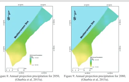
[image:3.595.325.501.296.527.2]In this research paper results of climate change projections were used from (Gharbia et al, 2015a), which presented a spatially distributed climate change projected maps for temperature and precipitation over Gaza Strip according to A1F1 with high sensitive case were developed based on baseline period maps for three time intervals (2020, 2050 and 2080) and used as input in this modeling work in order to investigate the impacts of climate change on water balance elements of the Gaza coastal area. The baseline period maps were prepared for temperature and precipitation for mean values from 1972 to 2002 as shown in Figure (2) & Figure (6). Fossil energy intensive (A1F1) with high sensitivity is the emission scenario that was used for the prediction process by SimCLIM climate model. The median assembly approach was used to get the representative results from multi General Circulation Model (GCM) outputs. As shown in Figures (3-5) the predicted mean annual temperatures for years 2020, 2050 and 2080 were 20.66 oC, 22.48 oC and 25.08 oC respectively, while 0.85 oC, 2.67 oC and 5.28 oC were the mean annual changes from baseline period for years 2020, 2050 and 2080 respectively. Figures (7-9) illustrate the predicted mean annual precipitation for years 2020, 2050 and 2080 were 294.68 mm/year, 243.70 mm/year and 170.82 mm/year respectively. Hence -7.48, -23.98 and -46.37 mm/year were the predicted mean annual precipitation changes from baseline period for years 2020, 2050 and 2080 respectively (Gharbia et al, 2015a).
Figure 2: Mean annual temperature (1972 – 2002), (Gharbia et al, 2015a).
[image:3.595.100.263.300.525.2]Figure 4: Mean annual projection temperature for 2050, (Gharbia et al, 2015a).
Figure 5: mean annual projection temperature for 2080, (Gharbia et al, 2015a).
Figure 6: Mean annual precipitation (mm) (1972 – 2002) , (Gharbia et al, 2015a).
Figure 8: Annual projection precipitation for 2050, (Gharbia et al, 2015a).
Figure 9: Annual projection precipitation for 2080, (Gharbia et al, 2015a).
2.3 Recharge prediction
Figure 10: Baseline period simulated mean annual groundwater recharge, (Gharbia et al, 2015b).
[image:6.595.299.487.380.633.2]Figure 11: Simulated mean annual groundwater recharge for year 2020, (Gharbia et al, 2015b).
Figure 12: Simulated mean annual groundwater recharge for year 2050, (Gharbia et al, 2015b).
Figure 13: Simulated mean annual groundwater recharge for year 2080, (Gharbia et al, 2015b).
2.4 Groundwater model
[image:6.595.80.271.381.633.2]scenario.
2.4.1 Model setup
The groundwater model domain encloses an area of 50 x 35 km in the south part of the regional coastal aquifer that includes the Gaza Strip coastal aquifer. The model domain is a uniform square grid comprising a grid spacing of 250x250m as shown in Figure (14). Only the east boundary was assigned as no flow boundary because of the end of the coastal aquifer boundary at this region and the start of the mountain aquifer (El-khalel Mountain). According to the geology of the coastal aquifer, a seven layer model elevation was established in order to simulate all of the sub aquifers and to be close to reality. The collected data contained partial data of all known wells in the period between 2004 and 2010, including the location of wells, coordinates, screens depths, abstractions. There is limited information about the well construction and pumping readings for illegally-dug wells which were discovered through a survey conducted lately by PWA. In the Gaza Strip area there were around 225 municipal wells in year (2010), about 2600 registered agricultural wells (PWA) and about 2900 illegal agriculture wells. The municipal wells were inserted into the model by their abstraction schedule, but the agricultural wells were inserted into the model by estimating their abstraction; these wells are shown in Figure (14). In the designed model 86 observation wells were inputted, this number represented the total number of the available observation wells in the Gaza strip for year 2010. In the designed model about 80 municipal wells were used as concentration observation wells. The horizontal hydraulic conductivity of the unsaturated zone for the soil types was assumed as 18 m/d for sand with fine gravel, 32 for sand stone and 0.3 m/d for clay. The vertical conductivity was set to 10% of the horizontal hydraulic conductivity. All of hydraulic properties and storage were set as shown in Table (2).
Table 2: Aquifer properties input values.
Parameter Sand with fine gravel Sandstone Clay
Hydraulic conductivity (m/d) Kh ,Kv 18 , 1.8 32 ,3.2 0.3 , 0.3
Specific storage (m-1) Ss 0.00001 0.00001 0.00001
Specific yield Sy 0.24 0.24 0.1
Effective porosity 0.25 0.25 0.4
Total porosity 0.3 0.3 0.45
The parameters that principally influence mass transport in the flow model are effective porosity and dispersivity. The effective porosity, ne, was set as in table 2; the uncertainty for the parameter was considered to be small, approx. 5 % (SWECO INT, 2003). Reducing (ne) will result in increased particle velocity which affects the time aspect in advective transport. Dispersivity was set to values ranging from 3 m to 12 m calculated by the following equation (SWECO INT, 2003):
DL=0.83 log L2.414 (1)
Where DL concerns longitudinal dispersivity and L is the length of the mass transport plume considered. Comparison of simulations showed that this difference in dispersivity did not result in any measurable changes of the diffusion plume.
Sea boundary was assumed constant head boundary. The illustrated results of sea level rise were assigned to the model as constant head boundary changing with time for the sea boundary.
In order to simulate the seawater intrusion phenomena, SEAWAT model was conduct using a constant salt concentration sea boundary. These constant concentrations may be as chloride or TDS (Total Dissolved Solids), a thirty sea water samples from each 1500 m of Gaza strip’s shore line was taken and analyzed, the chloride concentration ranges from 18637.5 to 24495 mg/l with a mean 23364.26 mg/l. This value was assigned as a constant concentration for sea boundary to the SEAWAT model.
Figure 14: Model Domain, pumping wells and cross section vertical layers.
2.4.2 Model calibration
[image:8.595.156.439.425.661.2]Data from year 2010 was used for the steady state calibration. The modeled water level was then calibrated based on the same year. Figure (15) compares the simulated results with the observed water level values. The modeled values show a correlation coefficient of 0.899 with the observed values with normalized RMS 8.665% which is less than 10% error: this value clearly demonstrates the high accuracy of the model. The SEAWAT model was calibrated for chloride concentration by entering the available chloride concentrations that were recorded for specific wells by PWA on year 2010. The model was run to get the simulated concentrations at year 2011 which was compared with PWA observed concentrations for the same year. This was done for each of the specific well locations to meet with the needed concentrations at year 2011. In addition the longitudinal dispersivity was adjusted since it is a required parameter for SEAWAT simulation as previously. As shown in Figure (16) it can be concluded that there is a very good match between the simulated and observed concentrations. The correlation coefficient is 0.888 between the simulated concentrations and the observed ones, and the Normalized RMS is 9.991% that is less than 10% error. It can be concluded that there is a very good match between the simulated and observed concentrations.
Figure 16: Concentration calibration results.
3. Results and Discussions
After setting up the groundwater MODFLOW model, calibrating and verification process, a Seawat transient groundwater model was run in order to determine the impacts of future predicted climate change condition. All of the previous predicted future climate conditions were used as input for this simulation process as discussed above. This section addresses the assessment of the impacts of future climate on groundwater level for the Gaza coastal aquifer. After the completion of the simulation process, results were explored for year’s interval 2015, 2020, 2025, 2030, 2050 and 2080. Figures (17-22) show the expected calculated head in the Gaza strip for years 2015, 2020, 2025, 2030, 2050 and 2080 respectively. It is observed that there are two cones of depression in the Gaza strip; one of them is in the north and the second is in the south. The head values in the north cone of depression decreases from -4.67 m at the middle in 2010 year to -4.697, -8.33, -8.419, -8.38, -10.414 and -12 meters at years 2015, 2020, 2025, 2030, 2050 and 2080 respectively. For the south cone of depression the head values decreases from –16.72 m at the middle in 2010 year to -17.7, -20.024, -21.118, -20.478 and -22.338 meters in years 2015, 2020, 2025, 2030, 2050 and 2080. Table (3) illustrates the simulated groundwater head raster maps statistics for years 2015, 2020, 2025, 2030, 2050, 2080.
Table 3: Predicted groundwater head raster maps statistics.
Item Head (MAX) MSL Head(MIN)MSL Head(MEAN)
MSL SD (MSL)
Y
ea
rs
2015 1.140 -17.650 -3.980 3.080
2020 1.090 -17.700 -4.050 3.060
2025 0.330 -21.040 -7.800 3.920
2030 0.290 -21.110 -7.900 3.900
2050 0.290 -21.330 -8.080 3.880
[image:9.595.66.533.528.674.2]The generated SEAWAT simulation process was used to determine the impacts of climate change on groundwater of the Gaza coastal aquifer mainly seawater intrusion phenomenon. The first simulation process was done without any management scenarios; Figures (24-29) illustrate the simulated chloride concentration for years 2015, 2020, 2025, 2030, 2050, 2080 respectively. The mean of each raster map chloride concentration is 1034.23, 1445.05, 2109.87, 2734.52, 4594.51, 7737.87 mg/l for years 2015, 2020, 2025, 2030, 2050, and 2080 respectively as shown in Table (4). All predicted chloride concentration maps show that only about 5% of the Gaza coastal aquifer has a chloride concentration less than 250 mg/l (WHO Standards). The generated chloride concentration profile shows that the chloride concentration dramatically increased with distance from the shoreline for each predicted successive year scenario. Figure (23) shows a randomly selected wells from each governorate in Gaza Strip with chloride concentration time series: all curves demonstrate that there is a rapid increase for chloride concentration with time.
[image:11.595.65.530.454.599.2]Figure 23: Simulated chloride concentration for number of selected wells. Table 4: Predicted Chloride concentration raster maps statistics.
Item Chloride (MAX)
mg/l Chloride(MIN)mg/l
Chloride(MEAN)
mg/l SD (mg/l)
Y
ea
rs
2015 23225.650 90.120 1034.230 2480.090
2020 23634.400 89.650 1445.050 3624.080
2025 23932.980 92.210 2109.870 4924.370
2030 24156.920 92.970 2734.520 5858.060
2050 24552.110 95.880 4594.510 7626.590
Gaza coastal aquifer can be adapted by climate changes impacts by management of pumping scenario and develop new water resources in order to conserve the aquifer from negative impacts or to minimize this impacts. The proposed solution scenario was actually based on the combination of seawater reverse osmosis desalination plant as part of Palestinian Water Authority (PWA) plan, of 55 Million cubic meter per year (Mm3) for the first phase is one of the proposed new water resources. By this quantity of high quality water, a possible envisaged solution would be to close a number of municipal pumping wells which have high salinity (1000 mg/l as chloride); after the closure of low water quality wells, a reduction in the pumping rate of other municipal wells must be done in order to achieve the total water quantity equal to the demand. The second step is to develop a new agricultural water resource, also according to (PWA) plans: by 2020 the utilization of wastewater is planned to provide 50 % of the total water required by agriculture, with the remainder being provided by the freshwater aquifer, in order to maintain the balance of salts in the soil and provide the quality necessary for certain crops (PWA, 2010). As such the agriculture wells will cease pumping in order to conserve the aquifer. The last step is to close the illegal commercial wells in Ariba area (21 wells) which are the main reason for developing the cone of depression in Rafah governorate. This proposed management scenario with all the steps above were developed in the same way of the construction of previous groundwater model in order to examine it as a complete solution to adapt with this high risk situation. The results for this model are as shown in Figurers (30 -33): the simulated groundwater head maps show that the maximum water head is -.98 , -0.99 , -1.03 and -3.4 m for years 2025, 2030, 2050 and 2080 respectively. By comparing these results with previous situation without any management scenario, for groundwater head parameter; this scenario is successful as a strategic solution. As shown in Table (5) the mean groundwater head for Gaza strip are 0.77, 0.75, 0.69 and -1.99 m for years 2025, 2030, 2050 and 2080 respectively.
Table 5: Predicted groundwater head raster maps statistics as results from management scenario.
By using the same developed groundwater model to examine the proposed management scenario, and after simulation for Seawat transient model, the results for proposed management scenario are shown in Figurers (34-37) and Table (6). The simulated chloride concentration maps show that the mean concentration is 723.51, 745.96, 917.77 and 2305.28 mg/l for years 2025, 2030, 2050 and 2080 respectively. By comparing these results with previous simulations without any management scenario, it can be understood that this scenario can be a strategic solution until year 2050, however it needs more developing in order to increase the sustainable situation of the aquifer.
Table 6: Predicted chloride concentration raster maps statistics as results from management scenario.
Item Chloride (MAX)
mg/l Chloride(MIN)mg/l Chloride(MEAN) mg/l SD (mg/l)
Y
ea
rs
2025 21396.140 83.910 723.500 1498.580
2030 21444.110 86.380 745.960 1616.330
2050 22749.130 79.380 917.770 2333.190
2080 23980.570 84.490 2305.280 5285.380
Item Head (MAX) MSL Head(MIN)MSL Head(MEAN) MSL SD (MSL)
Y
ea
rs
2025 3.110 -0.980 0.770 0.800
2030 3.100 -0.990 0.750 0.800
2050 3.060 -1.030 0.690 0.800
[image:13.595.61.536.604.713.2]Figure 30: Simulated Groundwater head by management scenario for year 2025.
Figure 31: Simulated Groundwater head by management scenario for year 2030.
Figure 32: Simulated Groundwater head by management scenario for year 2050.
Figure 34: Simulated Chloride concentration by
management scenario for 2025. Figure 35: Simulated Chloride concentration by management scenario for 2030.
Figure 36: Simulated Chloride concentration by
respectively. The mean predicted chloride concentration were 1034.23 mg/l, 1445.05 mg/l, 2109.8 mg/l, 2734.52 mg/l, 4594.51 mg/l and 7737.87 mg/l for years 2015, 2020, 2025, 2030, 2050 and 2080 respectively. From all generated chloride concentration profiles in the Gaza coastal aquifer, the concentration decreases by the increase of the distance from shoreline. An effective management scenario was developed and examined by the same groundwater transient model. The scenario was generated to adapt with climate change conditions by developing new water resources and managing pumping rate. This management scenario is a strategic solution for about thirty year period. Thedeveloped numerical groundwater model has shown that climate change will have severe negative impacts on the groundwater resource within the Gaza coastal aquifer.
Acknowledgment
I would like to express my sincere gratitude to Palestinian Water Authority (PWA) and CLIM systems Ltd. for the great support; I really want to thank Dr. Yinpeng Li for his help, Dr. Peter Urich for his continuous advice and Dr. Peter Kouwenhoven for his support.
References
Dettinger, M.D., Earman, S., 2007. Western ground water and climate change - pivotal to supply sustainability or vulnerable in its own right? Ground Water 4 (1), 4–5.
Elina C. , 2006, Seawater Intrusion in Complex Geological Environments, Department of Geotechnical Engineering and Geo-Sciences (ETCG), Technical University of Catalonia. Geneva. 210pp.
GOLDENBERG, L.C. (1992): Evaluation of the water balance in the Gaza Strip. Geological Survey, Report TR-GSI/16/92 (in Hebrew).
Gharbia S. Salem, Adnan Aish, Francesco Pilla, Abdalkarim S. Gharbia. “Projection of Future Climate by Multi-Model Median Approach under GIS Environment along the Gaza Strip, Palestine." Journal of
Environment and Earth Science (2015a).
Gharbia S. Salem, Adnan Aish, Francesco Pilla. “Impacts of Climate Change on a Spatially Distributed Water Balance in the Gaza Strip, Palestine" Journal of Environment and Earth Science (2015b).
GVIRTZMAN, G., SHACHNAI, E., BAKLER, N. & ILANI, S. (1984): Stratigraphy of the Kurkar group (Quaternary) of the coastal plain of Israel. Geological Survey of Israel, Current Research, 70–82.
JURY, W. & GARDNER, W. (1991): Soil physics. Fifth edition. ISBN: 0-471-83108-5, 4–18.
Jyrkama M. I., Jon F. Sykes, 2007, “The impact of climate change on spatially varying groundwater recharge in the Grand River watershed (Ontario), Journal of Hydrology (2007) 338, 237– 250.
MELLOUL, A.J. & COLLIN, M. (1994): The hydrological malaise of the Gaza Strip.– Isr. J. Earth Sci., 43/2, 105–116.
Naciri A, Ttlich G. Policy guidelines for wastewater management in the Gaza Strip. Potential of wastewater reuse in the Gaza Strip, 2001, p. 1–2.
Narula KK, Gosain AK., 2013, “Modeling hydrology, groundwater recharge and non-point nitrate loadings
in the Himalayan Upper Yamuna Basin”. Sci Total Environ 2013;468–469: S102–16.
http://dx.doi.org/10.1016/j.scitotenv.2013.01.022.
Palestinian Water Authority (PWA), 2012. Hydrogeological data bank department, Gaza Strip.
Palestinian Water Authority, 2000. Water Sector Strategic Planning Study.
Palestinian Water Authority, 2010. Agricultural & Municipal Water Consumption in Gaza Strip Report.
PCBS (2004).Palestinian Central Bureau of Statistics. Palestine in figures 2003, May 2004.
PHG (2002). Palestinian Hydrology Group for Water and Environmental Resources Development. Quality use of home reverse osmosis filters of some areas in Gaza Strip, 2002.
SWECO Annual Report 2003, SWECO, Stockholm.
Thuan Minh TRAN, 2004, “Multi-Objective Management of Saltwater Intrusion in Groundwater: