Antecedent Prediction Without a Pipeline
Sam Wiseman and Alexander M. Rush and Stuart M. Shieber
School of Engineering and Applied Sciences Harvard University
Cambridge, MA, USA
{swiseman,srush,shieber}@seas.harvard.edu
Abstract
We consider several antecedent prediction models that use no pipelined features gener-ated by upstream systems. Models trained in this way are interesting because they al-low for side-stepping the intricacies of up-stream models, and because we might expect them to generalize better to situations in which upstream features are unavailable or unreli-able. Through quantitative and qualitative er-ror analysis we identify what sorts of cases are particularly difficult for such models, and sug-gest some directions for further improvement.
1 Introduction
Most recent approaches to identity coreference reso-lution rely on a set of pipelined features generated by relatively accurate upstream systems. For instance, the CoNLL 2012 coreference datasets (Pradhan et al., 2012), which are based on the OntoNotes cor-pus (Hovy et al., 2006), make available both gold and predicted parse, part-of-speech, and named-entity information for each sentence in the corpus. While recent systems have managed to improve on the state of the art in coreference resolution by taking advantage of such information (Durrett and Klein, 2013; Wiseman et al., 2015; Bj¨orkelund and Kuhn, 2014; Fernandes et al., 2012; Martschat and Strube, 2015), we might be interested in systems that do not use pipelined features for several rea-sons: first, pipelined systems are known to accumu-late errors throughout the stages of the pipeline. Sec-ond, unpipelined models do not need to contend with the intricacies of the various systems in the pipeline,
which may have little impact on the target task. Fi-nally, models that do not require pipelined features may be more applicable to regimes in which up-stream features are unavailable or unreliable, such as those arising from predicting coreference in low-resource languages or in social media text. Indeed, to the extent that it is easier to obtain coreference annotations than it is to obtain (for instance) parse annotations in such regimes, an unpipelined strategy may be particularly practical.
Accordingly, in this paper we consider systems that attempt to move beyond OntoNotes by making coreference predictions without access to pipelined features, using only a document’s words and sen-tence boundaries. In the hopes of shedding light on whether this is a viable strategy, we consider, as a case study, how well coreference systems with-out access to upstream features can perform on En-glish. Given the amount of research that has gone into resolving English coreference resolution with pipelined features, by also considering the English “unpipelined” setting we can expect to get a rather accurate sense of how much we sacrifice by ignor-ing these features. Moreover, in addition to the ben-efits of unpipelined models noted above, the pro-posed line of research is congenial to the recent trend in NLP of using as few hand-engineered features as possible (as advocated, for instance, in Collobert et al. (2011)).
We report preliminary experiments on the subtask of antecedent prediction (defined in Wiseman et al. (2015) and reviewed below) on the CoNLL 2012 English dataset in this unpipelined setting. In par-ticular, we will assume that we have automatically
extracted mentions from a document, but that no other pipelined information is available. We empha-size that this is a strong assumption (since pipelined features, such as parse trees, are often used to ex-tract mentions), and so what follows should be in-terpreted as an attempt to obtain an upper bound on the performance possible in such a setting. We con-clude by analyzing the errors made by the proposed unpipelined systems, and discussing how these sys-tems might be made more competitive.
1.1 Problem Setting
As above, we will assume we are given a set of documents from which we are able to automati-cally extract mentions. We denote byX the set of these automatically extracted mentions. For a men-tionx∈ X, letA(x)denote the set of mentions ap-pearing before x in the document, and let the set C(x) ⊆ A(x) denote the mentions appearing be-fore x that are coreferent with x. The problem of antecedent ranking involves trying to predict an antecedent y ∈ C(x) for only those x for which C(x) 6= ∅, that is, for only thosexthat have coref-erent antecedents. We will moreover require that in making these antecedent predictions no pipelined features are used. In particular, we will assume that “unpipelined” systems have access only to a docu-ment’s mention-boundaries, to the setsC(x)for each
x∈ X (when training), to the words in each docu-ment, and to the document’s sentence boundaries.
Whereas recent coreference systems typically make use of syntactic information, named-entity tags, word-lists containing type information (e.g., number, gender, animacy), and speaker informa-tion (Durrett and Klein, 2013; Bj¨orkelund and Kuhn, 2014; Lee et al., 2013), given the aforementioned restrictions, the only common coreference features that remain legal are word-based features and “dis-tance” features. Distance features are typically de-fined in terms of the number of words, mentions, or sentences between a mention and a candidate an-tecedent (Durrett and Klein, 2013), and such fea-tures can presumably be defined accurately in many settings without the use of upstream systems.
2 Models
We will use a very simple mention-ranking style model for our antecedent prediction. Mention-ranking models make use of a scoring function
s(x, y)that scores the compatibility between a men-tionxand a candidate antecedenty, and they predict the antecedent to be y∗ = arg max
y∈C(x)s(x, y). We will definesas
s(x, y) =uTtanh W
ΦΦcc((xy))
Φd(x, y)
+b
,
where Φc extracts relevant word-based features
from a mention and its context, andΦdextracts
dis-tance based features between x and y. Thus, the scoring functionsis defined by applying a standard multi-layer perceptron (MLP) to the (vertically) con-catenated outputs of the functions Φc andΦd. In
particular, W represents the weight matrix of the MLP’s first hidden layer, bthe corresponding bias vector, and u the vector of weights projecting the first hidden layer into a scalar score. The exact di-mensions of these weights will become clear in what follows.
In definingΦcwe will view a mentionxspanning
M words as a sequence of real vectorsx1, . . . ,xM,
with eachxm∈RDobtained by looking up them’th
word in x in an embedding matrix E∈RD×|V|, where V is our fixed vocabulary. Accordingly, let X1:M∈RD×Mbe the matrix formed by
concatenat-ing the embeddconcatenat-ings of the words in a mention (in or-der). Analogously, letX−K:−1∈RD×Kbe the con-catenation of the embedding-vectors corresponding to the K words preceding x on the left (padded where necessary), andXM+1:M+K the
concatena-tion of the embedding-vectors corresponding to the
K words following x on the right (padded where necessary).
For simplicity, we will requireΦcto take the
fol-lowing form:
Φc(x) =
hh(X(X−1:KM:−1)) h(XM+1:M+k)
,
whereh(Xi:j)is some function of the matrixXi:j.
of the words ofxwith representations (respectively) of theKwords preceding and followingx.
For example, consider the following passage from the development portion of the CoNLL 2012 English development data, from which the final example in Table 1 is taken, and in which we have highlighted a particular mention we might like to predict an an-tecedent for:
Suddenly we realized water came into the engine room and it was rising and they started to pump, of course, and they pumped and pumped and the wa-ter came more and more and more. (bn/cnn/cnn 0410)
If we are interested in predicting coreferent an-tecedents for “the water,” which we will denote byx, then we will haveM= 2, andX1:2will be a matrix inRD×2 with its first column equal to the embed-ding (inE) for “the,” and its second column equal to the embedding for “water.” Since in predictingx
we will likely also want to take into account some of its surrounding context, we will also form matri-ces corresponding to theK words to the left and to the right (respectively) ofx. Thus, if we setK= 1, we will formX−1:−1 as the matrix inRD×1, which consists of the embedding for “and,” and we would define XM+1:M+1 analogously. Given the afore-mentionedX matrices, we defineΦc by vertically
concatenating the output of applying a functionhto each of these matrices.
We now consider three approaches to defining h(X1:M), in increasing order of complexity: Max-Over-Time Model: Defineh(X1:M)to be in
RD, with h(X
1:M)d = max1≤j≤M(X1:M)dj, for
eachd= 1, . . . , D.1
Convolutional Model: We follow Kim (2014) in generating F feature maps of M−h+ 1 features by applying a (non-linear) filter to each h-length window ofX1:M, and then max-pooling over time.
Thus,h(X1:M)∈RF.
LSTM Model: We define h(X1:M) to be in RH,
where h(X1:M) is the M’th hidden state of an
LSTM (Hochreiter and Schmidhuber, 1997) run over the vectorsx1, . . . ,xM inX1:M.
1We found the max-pooling described here to be more
ef-fective than mean-pooling.
To define Φd we first define indicator features
(represented as one-hot vectors), which (respec-tively) bucket the number of mentions and the num-ber of sentences between a mention and a candidate antecedent into 11 discrete buckets, following Dur-rett and Klein (2013). We therefore have 22 dis-tance indicator features in total, and they are used to index into an embedding matrix A∈RDd×22. Ac-cordingly,Φd(x, y)∈RDdrepresents the sum of the
(two) distance embeddings obtained fromAin this way. This approach resembles that of Sukhbaatar et al. (2015).
3 Experiments
3.1 Methods
We conduct antecedent-ranking experiments on the development portion of the CoNLL 2012 English corpus. Mentions were extracted using the Berke-ley Coreference System (Durrett and Klein, 2013). We set K= 4 in forming word-windows, and we trained by optimizing the margin ranking-loss de-fined in Wiseman et al. (2015) using mini-batch Adagrad (Duchi et al., 2011).
For the convolutional model, we used windows of size 1, 2, and 3, and 40 filters for each. We setDd,
the dimensionality of the distance feature embed-dings which constitute the columns ofA, to 20. We used theelement-rnnRNN package (L´eonard et al., 2015) to implement the LSTM, and we set the LSTM’s hidden-layer size to 200. All models used 300 hidden units in the final layer (represented by W), and we used Dropout for regularization. All hyperparameters including window size were tuned on the development set.
x Correct Antecedent Prediction Convolutional Antecedent Prediction the Straits [Foundation] the Straits [Foundation] the Straits [Association]
[image:4.612.115.259.168.238.2]those Jewish [sacrifices] the [sacrifices] the [people] of Israel the [water] [water] their sinking fishing [boat]
Table 1: Example mentions xwhich the baseline MLP correctly predicts (middle column), but the Convolutional Model (right column) does not. Heads of each mention (unseen by the Convolutional Model) are in brackets.
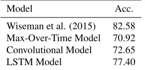
Model Acc.
Wiseman et al. (2015) 82.58 Max-Over-Time Model 70.92 Convolutional Model 72.65
LSTM Model 77.40
Table 2: Accuracy of models described in text (and base-line) on predicting antecedents on CoNLL Development set.
3.2 Results
We are particularly interested in determining in what situations a word-and-distance model under-performs models with access to more sophisticated information. In Table 2 we compare the antecedent-prediction accuracy of the three models defined above with the antecedent ranking performance of the model described in Wiseman et al. (2015), which uses an MLP over pipelined coreference features. We will refer to this latter model as the “base-line MLP.” We see that the word-and-distance mod-els underperform, though the LSTM model comes within 5.2% of the baseline MLP. (It is also worth noting here that without the distance featuresΦdall
models are significantly less accurate, with accura-cies decreasing by over 15 percentage points). 4 Discussion
In Table 3 we examine, using an analysis simi-lar to that in Durrett and Klein (2013), where the unpipelined models go wrong. There, we parti-tion menparti-tions column-wise into nominal or proper mentions that have a head-match with some previ-ously occurring mention, nominal or proper men-tions that do not, and pronominal menmen-tions. (Note that whereas parse information must be used to de-tect heads, this is only used in our analysis, and none of the three models introduced here have access to this information).
Let us first consider the Convolutional Model,
Errors
HM No HM Pron. Wiseman et al. (2015) 588 522 1146 Max-Over-Time Model 1513 608 1646 Convolutional Model 1358 607 1577
LSTM Model 1028 537 1362
Total Mentions 4677 973 7302 Table 3: Errors of models described in text on CoNLL 2012 development set. Mentions are partitioned column-wise as nominal or proper with (previous) head match in the document (HM), nominal or proper with no previous head match in the document (No HM), and pronominal.
which underperforms the baseline in all categories, but does particularly badly in predicting antecedents for mentions for which a previous mention in the text has the same head.
Why is this? Further analysis shows that almost 84% of the HM examples that are correctly predicted by the baseline MLP but incorrectly predicted by the Convolutional Model involve the baseline MLP pre-dicting an antecedent with an exact head-match to the current mention, and the Convolutional Model predicting a non-head-match antecedent. We show some representative examples in Table 1, where we bracket the head of each mention. As is evident from Table 1, the model is picking antecedents that are semantically reasonable, but which do not have a head match. The reason the Convolutional Model makes these errors is presumably that it is not able to tell what the head of each mention is (because it sees only the words in the mention, and the word-windows preceding and following). The baseline MLP, however, does have access to the heads of each mention, and so can learn that head-match is a dis-criminative feature.
Figure 1: Percentage of antecedents in the CoNLL 2012 development set predicted correctly, by mention length.
model’s errors in the HM category also involve predicting a non-head-match antecedent when the baseline MLP correctly predicts a head-match an-tecedent. Thus, it seems the LSTM model too could benefit from better head-finding. As additional ev-idence for this hypothesis, in Figure 1 we plot the percentage of correctly predicted antecedents in the CoNLL 2012 development set as the length of the current mentionxincreases. (Only mention-lengths occurring≥10times in the development set are re-ported). We see that the accuracy of both the Con-volutional and LSTM models (as well as that of the Max-Over-Time model) generally decreases as the mention-length increases, though that of the base-line MLP model does not. Of course, it stands to reason that finding heads is more difficult in longer mentions, which may explain this trend.
When it comes to the other major category of errors in Table 3, namely, errors on pronominal mentions, it is more difficult to diagnose a single underlying cause of error. In particular, the un-pipelined models’ errors tend to involve either pre-dicting antecedents that are inconsistent in terms of gender or number, or, interestingly, predicting non-pronominal antecedents when the baseline MLP pre-dicts a pronominal antecedent. While it is certainly the case that the baseline MLP has access to gender information that the unpipelined models do not, it is not as clear why these unpipelined models learn to disprefer predicting pronominal antecedents for pronominal mentions, and this issue requires further investigation.
5 Conclusion
The results presented above suggest that a major factor holding word-and-distance-only models back from competing with models that have access to pipelined features is their inability to find mention-heads and, more generally, to take advantage of syn-tactic features. While the fact that such models would benefit from syntactic information is not sur-prising, the examples in Table 1 suggest that even coarse notions of head-finding may be sufficient to improve performance. Accordingly, one might imagine that alignment or attention models (such as that of Bahdanau et al. (2014)) that attempt to model coarse head-information would be useful in such cases.
References
Dzmitry Bahdanau, Kyunghyun Cho, and Yoshua Ben-gio. 2014. Neural machine translation by jointly learning to align and translate. arXiv preprint arXiv:1409.0473.
Anders Bj¨orkelund and Jonas Kuhn. 2014. Learning structured perceptrons for coreference Resolution with Latent Antecedents and Non-local Features. ACL, Baltimore, MD, USA, June.
Ronan Collobert, Jason Weston, L´eon Bottou, Michael Karlen, Koray Kavukcuoglu, and Pavel Kuksa. 2011. Natural Language Processing (almost) from Scratch.
The Journal of Machine Learning Research, 12:2493– 2537.
John Duchi, Elad Hazan, and Yoram Singer. 2011. Adaptive Subgradient Methods for Online Learning and Stochastic Optimization. The Journal of Machine Learning Research, 12:2121–2159.
Greg Durrett and Dan Klein. 2013. Easy Victories and Uphill Battles in Coreference Resolution. In Proceed-ings of the 2013 Conference on Empirical Methods in Natural Language Processing, pages 1971–1982. Eraldo Rezende Fernandes, C´ıcero Nogueira Dos Santos,
and Ruy Luiz Milidi´u. 2012. Latent Structure Per-ceptron with Feature Induction for Unrestricted Coref-erence Resolution. In Joint Conference on EMNLP and CoNLL-Shared Task, pages 41–48. Association for Computational Linguistics.
Sepp Hochreiter and J¨urgen Schmidhuber. 1997. Long short-term memory.Neural Comput., 9:1735–1780. Eduard Hovy, Mitchell Marcus, Martha Palmer, Lance
Compan-ion Volume: Short Papers, pages 57–60. Association for Computational Linguistics.
Yoon Kim. 2014. Convolutional neural networks for sen-tence classification. InProceedings of the 2014 Con-ference on Empirical Methods in Natural Language Processing, EMNLP, pages 1746–1751.
Heeyoung Lee, Angel Chang, Yves Peirsman, Nathanael Chambers, Mihai Surdeanu, and Dan Jurafsky. 2013. Deterministic Coreference Resolution based on Entity-centric, Precision-ranked Rules. Computational Lin-guistics, 39(4):885–916.
Nicholas L´eonard, Yand Waghmare, Sagar ad Wang, and Jin-Hwa Kim. 2015. rnn: Recurrent Library for Torch. arXiv preprint arXiv:1511.07889.
Sebastian Martschat and Michael Strube. 2015. Latent structures for coreference resolution. TACL, 3:405– 418.
Tomas Mikolov, Ilya Sutskever, Kai Chen, Greg S Cor-rado, and Jeff Dean. 2013. Distributed representa-tions of words and phrases and their compositionality. InAdvances in neural information processing systems, pages 3111–3119.
Sameer Pradhan, Alessandro Moschitti, Nianwen Xue, Olga Uryupina, and Yuchen Zhang. 2012. Conll-2012 Shared Task: Modeling Multilingual Unre-stricted Coreference in OntoNotes. In Joint Confer-ence on EMNLP and CoNLL-Shared Task, pages 1–40. Association for Computational Linguistics.
Sainbayar Sukhbaatar, Jason Weston, Rob Fergus, et al. 2015. End-to-end memory networks. InAdvances in Neural Information Processing Systems, pages 2431– 2439.