Generalization in Artificial Language Learning: Modelling the Propensity to Generalize

Generalization in Artificial Language Learning:

Modelling the Propensity to Generalize

Raquel G. Alhama, Willem Zuidema

Institute for Logic, Language and Computation University of Amsterdam, The Netherlands

{rgalhama, w.h.zuidema}@uva.nl

Abstract

Experiments in Artificial Language Learn-ing have revealed much about the cogni-tive mechanisms underlying sequence and language learning in human adults, in in-fants and in non-human animals. This pa-per focuses on their ability to generalize to novel grammatical instances (i.e., in-stances consistent with a familiarization pattern). Notably, the propensity to gen-eralize appears to be negatively correlated with the amount of exposure to the artifi-cial language, a fact that has been claimed to be contrary to the predictions of statis-tical models (Pe˜na et al. (2002); Endress and Bonatti (2007)). In this paper, we pro-pose to model generalization as a three-step process, and we demonstrate that the use of statistical models for the first two steps, contrary to widespread intuitions in the ALL-field, can explain the observed decrease of the propensity to generalize with exposure time.

1 Introduction

In the last twenty years, experiments in Artificial Language Learning (ALL) have become increas-ingly popular for the study of the basic mecha-nisms that operate when subjects are exposed to language-like stimuli. Thanks to these experi-ments, we know that 8 month old infants can seg-ment a speech stream by extracting statistical in-formation of the input, such as the transitional probabilities between adjacent syllables (Saffran et al. (1996a); Aslin et al. (1998)). This ability also seems to be present in human adults (Saffran et al., 1996b), and to some extent in nonhuman animals like cotton-top tamarins (Hauser et al., 2001) and rats (Toro and Trobal´on, 2005).

Even though this statistical mechanism is well attested for segmentation, it has been claimed that it does not suffice for generalization to novel stimuli or rule learning1_{. Ignited by a}

study by Marcus et al. (1999), which postu-lated the existence of an additional rule-based mechanism for generalization, a vigorous debate emerged around the question of whether the ev-idence from ALL-experiments supports the exis-tence of a specialized mechanism for generaliza-tion (Pe˜na et al. (2002); Onnis et al. (2005); En-dress&Bonatti (2007); Frost&Monaghan (2016); Endress&Bonatti (2016)), echoing earlier debates about the supposed dichotomy between rules and statistics (Chomsky, 1957; Rumelhart and Mc-Clelland, 1986; Pinker and Prince, 1988; Pereira, 2000).

From a Natural Language Processing perspec-tive, the dichotomy between rules and statistics is unhelpful. In this paper, we therefore pro-pose a different conceptualization of the steps in-volved in generalization in ALL. In the follow-ing sections, we will first review some of the ex-perimental data that has been interpreted as ev-idence for an additional generalization mecha-nism (Pe˜na et al. (2002); Endress&Bonatti (2007); Frost&Monaghan (2016)). We then reframe the interpretation of those results with our 3-step ap-proach, a proposal of the main steps that are re-quired for generalization, involving: (i) memo-rization of segments of the input, (ii) computa-tion of the probability for unseen sequences, and (iii) distribution of this probability among partic-ular unseen sequences. We model the first step with the Retention&Recognition model (Alhama et al., 2016). We propose that a rational

charac-1_{We prefer the term ‘generalization’ because}

‘rule-learning’ can be confused with a particular theory of gen-eralization that claims that the mental structures used in the generalization process have the form of algebraic rules.

terization of the second step can be accomplished with the use ofsmoothing techniques (which we further demonstrate with the use of the Sim-ple Good-Turing method, (Good&Turing (1953); Gale (1995)). We then argue that the modelling results shown in these two steps already account for the key aspects of the experimental data; and importantly, it removes the need to postulate an additional, separate generalization mechanism.

2 Experimental Record

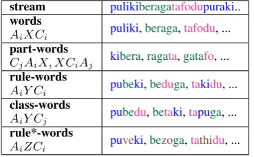
Pe˜na et al. (2002) conduct a series of Artificial Language Learning experiments in which French-speaking adults are familiarized to a synthesized speech stream consisting of a sequence of artificial words. Each of these words contains three sylla-bles AiXCi such that the Ai syllable always

co-occurs with the Ci syllable (as indicated by the

subindex i). This forms a consistent pattern (a “rule”) consisting in a non-adjacent dependency betweenAi andCi, with a middle syllableXthat

varies. The order of the words in the stream is randomized, with the constraint that words do not appear consecutively if they either: (i) belong to the same “family” (i.e., they have the sameAiand

Ci syllables), or (ii) they have the same middle

syllableX.

stream pulikiberagatafodupuraki..

words

AiXCi puliki,beraga,tafodu, ...

part-words

CjAiX, XCiAj kibera,ragata,gatafo, ...

rule-words

AiY Ci pubeki,beduga,takidu, ...

class-words

AiY Cj pubedu,betaki,tapuga, ...

rule*-words

AiZCi puveki,bezoga,tathidu, ... Table 1: Summary of the stimuli used in the de-picted experiments.

After the familiarization phase, the participants respond a two-alternative forced choice test. The two-alternatives involve a word vs. a part-word, or a word vs. arule-word, and the participants are asked to judge which item seemed to them more like a word of the imaginary language they had listened to. A part-word is an ill-segmented se-quence of the form XCiAj orCiAjX; a choice

for a part-word over a word is assumed to indicate that the word was not correctly extracted from the stream. A rule-word is a rule-obeying sequence that involves a “novel” middle syllableY

(mean-ing thatY did not appear in the stream as anX, al-though it did appear as anAorC). Rule-words are therefore a particular generalization from words. Table 1 shows examples of these type of test items. In their baseline experiment, the authors expose the participants to a 10 minute stream ofAiXCi

words. In the subsequent test phase, the sub-jects show a significant preference for words over part-words, proving that the words could be seg-mented out of the familiarization stream. In a sec-ond experiment the same setup is used, with the exception that the test now involves a choice be-tween a part-word and a rule-word. The subjects’ responses in this experiment do not show a sig-nificant preference for either part-words or rule-words, suggesting that participants do not gener-alize to novel grammatical sequences. However, when the authors, in a third experiment, insert mi-cropauses of 25ms between the words, the partic-ipants do show a preference for rule-words over part-words. A shorter familiarization (2 minutes) containing micropauses also results in a prefer-ence for rule-words; in contrast, a longer familiar-ization (30 minutes) without the micropauses re-sults in a preference for part-words. In short, the presence of micropauses seems to facilitate gener-alization to rule-words, while the amount of expo-sure time correlates negatively with this capacity.

Endress and Bonatti (2007) report a range of ex-periments with the same familiarization procedure used by Pe˜na et al. However, their test for general-ization is based onclass-words: unseen sequences that start with a syllable of class “A” and end with a syllable of class “C”, but withAandC not ap-pearing in the same triplet in the familiarization (and therefore not forming a nonadjacent depen-dency).

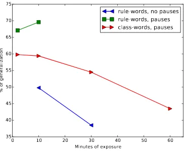
From the extensive list of experiments con-ducted by the authors, we will refer only to those that test the preference between words and class-words, for different amounts of exposure time. The results for those experiments (illustrated in figure 1) also show that the preference for general-ized sequences decreases with exposure time. For short exposures (2 and 10 minutes) there is a sig-nificant preference for class-words; when the ex-posure time is increased to 30 minutes, there is no preference for either type of sequence, and in a 60 minutes exposure, the preference reverses to part-words.

0 10 20 30 40 50 60 Minutes of exposure

35 40 45 50 55 60 65 70 75

% of generalization

rule-words, no pauses rule-words, pauses class-words, pauses

Figure 1: Percentage of choices for rule-words and class-words, in the experiments reported in Pe˜na et al. (2002) and Endress&Bonatti (2007), for differ-ent exposure times to the familiarization stream.

micropauses are not essential for rule-like general-ization to occur. Rather, the degree of generaliza-tion depends on the type of test sequences. The authors notice that the middle syllables used in rule-words might actually discourage generaliza-tion, since those syllables appear in a different po-sition in the stream. Therefore, they test their par-ticipants withrule*-words: sequences of the form AiZCi, where Ai andCi co-occur in the stream,

andZdoes not appear. After a 10 minute exposure without pauses, participants show a clear prefer-ence for the rule*-words over part-words of the formZCiAj orCiAjZ.

The pattern of results is complex, but we can identify the following key findings: (i) general-ization for a stream without pauses is only man-ifested for rule*-words, but not for rule-words nor class-words; (ii) the preference for rule-words and class-words is boosted if micropauses are present; (iii) increasing the amount of exposure time corre-lates negatively with generalization to rule-words and class-words (with differences depending on the type of generalization and the presence of mi-cropauses, as can be seen in figure 1). This last phenomenon, which we call time effect, is pre-cisely the aspect we want to explain with our model. (Note, in figure 1, that in the case of rule-words and pauses, the amount of generalization in-creases a tiny bit with exposure time, contrary to the time effect. We cannot test whether this is a significant difference, since we do not have access to the data. Endress&Bonatti, however, provided convincing statistical analysis supporting a

signif-icant inverse correlation between exposure time and generalization to class-words).

3 Understanding the generalization mechanism: a 3-step approach

Pe˜na et al. interpret their findings as support for the theory that there are at least two mechanisms, which get activated in the human brain based on different cues in the input. Endress and Bonatti adopt that conclusion (and name it the

More-than-One-Mechanismhypothesis, or MoM), and

more-over claim that this additional mechanism cannot be based on statistical computations. The authors predict that statistical learning would benefit from increasing the amount of exposure:

“If participants compute the generaliza-tions by a single associationist mecha-nism, then they should benefit from an increase in exposure, because longer experience should strengthen the rep-resentations built by associative learn-ing (whatever these representations may be).” (Endress and Bonatti, 2007)

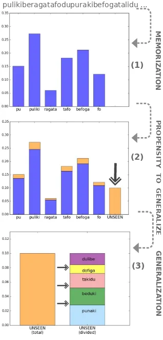
We think this argument is based on a wrong premise: stronger representations do not necessar-ily entail greater generalization. On the contrary, we argue that even very basic models of statisti-cal smoothing make the opposite prediction. To demonstrate this in a model that can be compared to empirical data, we propose to think about the process of generalization in ALL as involving the following steps (illustrated also in figure 2):

(i) Memorization: Build up a memory store of segments with frequency information (i.e., compute subjective frequencies).

(ii) Quantification of the propensity to gener-alize: Depending on the frequency informa-tion from (i), decide how likely are other un-seen types.

(iii) Distribution of probability over possible generalizations: Distribute the probability for unseen types computed in (ii), assigning a probability to each generalized sequence.

pulikiberagatafodupurakibefogatalidu ...

(1)

(3) (2)

M

E

M

O

R

IZ

A

T

IO

N

G

E

N

E

R

A

L

IZ

A

T

IO

N

P

R

O

P

E

N

S

IT

Y

T

O

G

E

N

E

R

A

L

IZ

E

Figure 2: Three step approach to generalization: (1) memorization of segments, (2) compute prob-ability of new items, and (3) distribute probprob-ability between possible new items.

not only based on the particular structure underly-ing the stimuli, but also depends on the statistical properties of the input.

At this point, we can already reassess the MoM hypothesis: more exposure time does entail bet-ter representation of the stimuli (as would be re-flected in step (i)), but the impact of exposure time on generalization depends on the model used for step (ii). Next, we show that a cognitive model of step (i) and a rational statistical model of step (ii) already account for thetime effect.

4 Memorization of segments: the Retention and Recognitionmodel

For step (i) of our approach, several existing models maybe used, including models based on recurrent neural networks (Seidenberg and El-man, 1999), autoencoders (French et al., 2011; French and Cottrell, 2014), exemplar-based

pro-cessing (Perruchet and Vinter, 1998) and non-parametric Bayesian inference (Goldwater et al., 2006). We have decided to implement the Re-tention&Recognition (R&R) model, proposed in (Alhama et al., 2016). R&R is a probabilistic exemplar-based model that has been shown to fit experimental data from a range of ALL exper-iments on segmentation, and, importantly, pro-duces very skewed frequency distributions that fit well with our intuition about step (ii).

Starting from an initially empty memory, R&R processes subsequences (segments) of the speech stream, and decides probabilistically whether those segments will be stored in its internal mem-ory. The output of the model is a memory of seg-ments, each one with a count of how many times the model has decided to store it in memory. The authors refer to these counts assubjective frequen-cies.

In each iteration, R&R is presented with one segment from the input stream. Each segment may be composed of any number of syllables (un-til an arbitrarily set maximum). For instance, for a stream starting with talidupuraki..., the model would be presented, in order, with the segmentsta, tali, talidu, talidupu, li, lidu, lidupu, lidupura, etc. (assuming a maximum length of four syllables).

Each one of these segments is processed as shown in figure 3: first, the recognition mecha-nism attempts to recognize the segment (that is, it attempts to determine whether the segment cor-responds to one of the segments already in mem-ory). If the attempt succeeds, the subjective fre-quency (count) of the segment in memory is in-creased with one. If the segment was not recog-nized, the model may still retain it. If it does, the segment will be added to the memory (or, if al-ready there from a previous iteration, its subjec-tive frequency is increased with one). If not, the segment is ignored, and the next segment is pro-cessed.

The recognition probability p1for segmentsis

defined as follows (eq. 1):

p1(s) = (1−Bactivation(s))·D#types (1)

06B, D61

subjec-NOT RETAINED pulikiberagatafodupurakibefogatalidu ...

pu puli puliki pulikibe li liki likibe likibera ki kibe kibera kiberaga ...

SEGMENTS (for max. length 4): STREAM:

segment s

RETA INED RECOGNIZED NOT RECOGNIZED

RECOGNITION p₁(s)

RETENTION p₂(s)

Increment subjective frequency of s

Ignore s

Figure 3: The Retention&Recognition model. Diagram based on Alhama et al. (2016).

tive frequency are easier to recognize. However, the number of different segment types in memory (#types) makes the recognition task more diffi-cult.

The retention probabilityp2is defined in eq. 2:

p2(s) =Alength(s)·Cπ (2)

06A, C 61; π=

0after a pause 1otherwise

A andC are parameters to be set with empirical data, and π takes the value 0 when the segment being processed occurs right after a pause, and 1 otherwise. The retention probability is greater for shorter segments (as can be deduced from the

length(s)exponent applied to an A parameter that

ranges between 0 and 1). TheCparameter, which is again between 0 and 1, attenuates this proba-bility unless a pause precedes the segment. This has the effect of boosting the retention of segments that appear after a pause.

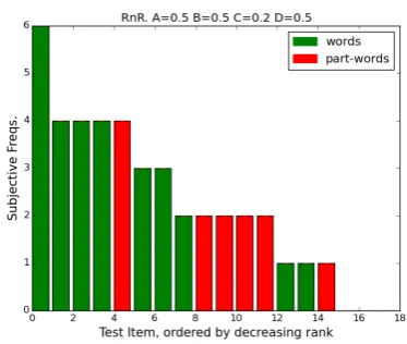
The four parameters involved in the model (A, B, C, D) set the contribution of each of its components, and allow for the adaptation of the model to different tasks or species. Alhama et al. did not report the optimal parameter setting for the experiments we are concerned with here, but they assert that the main qualitative features of the model (such as the rich-get-richer dynamics of the recognition function) are independent of the parameters.

Among these qualitative features, one that is particularly relevant for our study is theskewthat can be observed in the subjective frequencies com-puted by the model. This feature, which can be observed in figure 4, is presented in the original paper as being in consonance with empirical data. Here, we show that this property can also be val-idated in a different way: when R&R is part of a pipeline of models (like the 3-step approach), the skew turns out to be a necessary property for the success of the next model in the sequence. We come back to this point in section 7.

5 Quantifying the propensity to generalize: the Simple Good-Turing method

In probabilistic modelling, generalization must necessarily involve shifting probability mass from attested events to unattested events. This is a well known problem in Natural Language Processing, and the techniques to deal with it are known as smoothing. Here, we explore the use of the Simple Good Turing (Gale and Sampson, 1995) smooth-ing method as a computational level characteriza-tion of the propensity to generalize.

Simple Good-Turing (SGT), a computation-ally efficient implementation of the Good-Turing method (Good, 1953), is a technique to estimate the frequency of unseen types, based on the fre-quency of already observed types. The method works as follows: we take the subjective frequen-cies r computed by R&R and, for each of them, we compute the frequency of that frequency (Nr),

that is, the number of sequences that have a cer-tain subjective frequency r. The values Nr are

then smoothed, that is re-estimated with a

con-tinuous downward-sloping line in log space. The smoothed valuesS(Nr)are used to reestimate the

frequencies according to (3):

r∗ _{= (r+ 1)}S(Nr+1)

S(Nr) (3)

The probabilities for frequency classes are then computed based on these reestimated frequencies:

pr = r

∗

N (4)

where N is the total of the unnormalized esti-mates2_.

Finally, the probability for unseen events is computed based on the (estimated)3_{probability of}

types of frequency one, with the following equa-tion:

P0= S(_NN1) (5)

This probability P0 corresponds to what we

have called “propensity to generalize”.

2_{It should be noticed that the reestimated probabilities}

need to be renormalized to sum up to 1, by multiplying with the estimated total probability of seen types1−P0 and di-viding by the sum of unnormalized probabilites.

3_{SGT incorporates a rule for switching betweenN}

r and

S(Nr)such that smoothed valuesS(Nr)are only used when they yield significantly different results fromNr (when the difference is greater than 1.96 times the standard deviation).

As can be deduced from the equations, SGT is designed to ensure that the probability for unseen types is similar to the probability of types with fre-quency one. The propensity to generalize is there-fore greater for distributions where most of the probability mass is for smaller frequencies. This obeys a rational principle: when types have been observed with high frequency, it is likely that all the types in the population have already been at-tested; on the contrary, when there are many low-frequency types, it may be expected that there are also types not yet attested.

6 Results

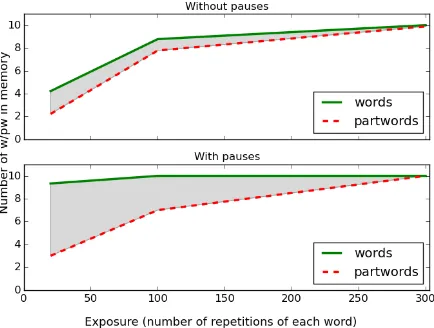
6.1 Memorization of words and part-words First we analyze the effect of the different condi-tions (exposure time and presence of pauses) in the memorization of segments computed with R&R (step (i)). Figure 5 shows the presence of test items (the nine words and nine possible part-words) in the memory of R&R after different exposure times (average out of ten runs of the model). As can be seen, the subjective frequencies of part-words in-crease over time, and thus, the difference between words and part-words decreases as the exposure increases.

Figure 5: Average number of memorized words and part-words after familiarization with the stim-uli in Pe˜na et al., for 10 runs of the R&R model with an arbitrary parameter setting (A=0.5 B=0.5 C=0.2 D=0.5).

The results of these simulations are consistent with the experimental results: the choice for words (or sequences generalized from words) against part-words should benefit from shorter exposures and from the presence of the micropauses. Now, given the subjective frequencies, how can we com-pute the propensity to generalize?

6.2 Prediction of observed decrease in the propensity to generalize

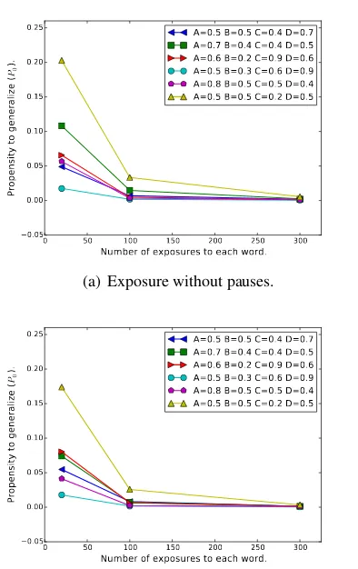
Next, we apply the Simple Good-Turing method4

to subjective frequencies computed by the R&R model. As shown in figure 6, we find that the propensity to generalize (P0) decreases as the

ex-posure time increases, regardless of the parameter setting used in R&R. This result is consistent with the rationale in the Simple Good-Turing method: as exposure time increases, frequencies are shifted to greater values, causing a decrease in the smaller frequencies and therefore reducing the expectation for unattested sequences.

The results of these simulations point to a straightforward explanation of the experimental finding of a reduced preference for the generalized sequences: longer exposures repeat the same set of words (and partwords), and consequently, par-ticipants may conclude that there are no other se-quences in that language – otherwise they would have probably appeared in such a long language sample.

It can be noticed in the graphs that the propen-sity to generalize is slightly smaller for the mi-cropause condition. The reason for that is that R&R identifies words faster when micropauses are present, and therefore, the subjective frequen-cies tend to be greater. This might appear unex-pected, but it is in fact not contradicting the em-pirical results: as shown in figure 5, the differ-ence between words and partwords is much big-ger in the condition with micropauses, so this ef-fect is likely to override the small probability dif-ference (as would be confirmed by a model of step (iii)). It should be noted that, as reported in Frost&Monaghan (2016), micropauses are not essential for all type of generalizations (as is ev-idenced with the fact that rule*-words are gener-alized in the no-pause condition). Like those au-thors, we see as the role of the micropauses to en-hance the salience of initial and final syllables (A

4_{We use the free software implementation of Simple Good}

Turing in https://github.com/maxbane/simplegoodturing.

0 50 100 150 200 250 300

Number of exposures to each word.

0.05 0.00 0.05 0.10 0.15 0.20 0.25

Pr

op

en

sit

y t

o g

en

er

ali

ze

(

P0

).

A=0.5 B=0.5 C=0.4 D=0.7 A=0.7 B=0.4 C=0.4 D=0.5 A=0.6 B=0.2 C=0.9 D=0.6 A=0.5 B=0.3 C=0.6 D=0.9 A=0.8 B=0.5 C=0.5 D=0.4 A=0.5 B=0.5 C=0.2 D=0.5

(a) Exposure without pauses.

0 50 100 150 200 250 300

Number of exposures to each word.

0.05 0.00 0.05 0.10 0.15 0.20 0.25

Pr

op

en

sit

y t

o g

en

er

ali

ze

(

P0

).

A=0.5 B=0.5 C=0.4 D=0.7 A=0.7 B=0.4 C=0.4 D=0.5 A=0.6 B=0.2 C=0.9 D=0.6 A=0.5 B=0.3 C=0.6 D=0.9 A=0.8 B=0.5 C=0.5 D=0.4 A=0.5 B=0.5 C=0.2 D=0.5

(b) Exposure with pauses.

Figure 6: Propensity to generalize, for several pa-rameter settings (average of 100 runs). Our model shows a clear decrease for all parameter settings we tried, consistent with the empirical data (com-pare with figure 1).

and C) to compensate for the odd construction of the test items (rule-words and class-words), which include a middle syllable that occupied a different position in the familiarization stream.

7 Discussion

distribu-tion of subjective frequencies that is crucial for step (ii); and third, with the Simple Good-Turing method for quantifying the propensity to general-ize. We now discuss how we interpret the outcome of our study.

Framing generalization with the 3-step ap-proach allowed us to identify a step that is usu-ally neglected in discussion of ALL, namely, the computation of the propensity to generalize. We state that generalization is not only a process of discovering structure: the frequencies in the famil-iarization generate an expectation about the prob-ability of next observing any unattested item, and the responses for generalized sequences must be affected by it. Moreover, this step is based on sta-tistical information, proving that — contrary to the MoM hypothesis — a statistical mechanism can account for the negative correlation with exposure time.

It should be noted that our conclusion concerns the qualitative nature of the learning mechanism that is responsible for the experimental findings. It has been postulated that such findings evidence the presence ofmultiplemechanisms (Endress and Bonatti, 2016). In our view, the notion of ‘mecha-nism’ is only meaningful as a high-level construct that may help researchers in narrowing down the scope of the computations that are being studied, among all the computations that take place in the brain at a given time. After all, there is no nat-ural obvious way to isolate the computations that would constitute a single ‘mechanism’, from an implementational point of view. Therefore, our 3-step approach should be taken as sketching the as-pects that any model of generalization should ac-count for, and our modelling efforts show that the experimental results are expected given the statis-tical properties of the input.

One issue to discuss is the influence of the use of the R&R model in computing the propensity to generalize. The Simple Good-Turing method is designed to exploit the fact that words in natu-ral language follow a Zipfian distribution —that is, languages consist of a few highly frequent words and a long tail of unfrequent words. This is a key property of natural language that is normally vio-lated in ALL experiments, since most of the arti-ficial languages used are based on a uniform dis-tribution of words (but see Kurumada et al. 2013). But it would be implausible to assume that sub-jects extract the exact distribution for an unknown

artificial language to which they have been only briefly exposed. R&R models the transition from absolute to subjective frequencies, resulting in a distribution of subjective frequencies that shows a great degree of skew, and much more so than al-ternative models of segmentation in ALL. Thanks to this fact, the frequency distribution over which the SGT method operates (the subjective distribu-tion) is more similar to that of natural language, and the pattern of results found for the propensity to generalize crucially depends on this type of dis-tribution.

Finally, we have thus accomplished our goal qualitatively. We capture the downward tendency of the propensity to generalize, but a model for step (iii), a longstanding question in linguistics and cognitive science, is required to also achieve a quantitative fit. Developing a model of step (iii) is left as future work, but our approach already al-lowed us to propose concrete models of the first two steps, and explain much of the pattern of re-sults.

Acknowledgments

This work was developed with Remko Scha, who sadly passed away before the finalization of this paper. We thank Carel ten Cate, Clara Levelt, Andreea Geambasu and Michelle Spierings for their feedback. We are also grateful to Raquel Fern´andez, Stella Frank and Miloˇs Stanojevi´c for their comments on the paper. This research was funded by NWO (360-70-450).

References

Raquel G. Alhama, Remko Scha, and Willem Zuidema. 2016. Memorization of sequence-segments by humans and non-human animals: the retention-recognition model. ILLC Prepublications, PP-2016-08.

Richard N Aslin, Jenny R Saffran, and Elissa L New-port. 1998. Computation of conditional probability statistics by 8-month-old infants. Psychological Sci-ence, 9(4):321–324.

Noam Chomsky. 1957. Syntactic Structures. Mouton, The Hague.

A.D. Endress and L.L. Bonatti. 2007. Rapid learning of syllable classes from a perceptually continuous speech stream. Cognition, 105(2):247–299. A.D. Endress and L.L. Bonatti. 2016. Words, rules,

Robert M French and Garrison W Cottrell. 2014. Tracx 2.0: A memory-based, biologically-plausible model of sequence segmentation and chunk extrac-tion. Proceedings of the 36th Annual Conference of the Cognitive Science Society.

Robert M. French, Caspar Addyman, and Denis Mareschal. 2011. Tracx: A recognition-based connectionist framework for sequence segmenta-tion and chunk extracsegmenta-tion. Psychological Review, 118(4):614.

Rebecca LA Frost and Padraic Monaghan. 2016. Simultaneous segmentation and generalisation of non-adjacent dependencies from continuous speech.

Cognition, 147:70–74.

W. A. Gale and G. Sampson. 1995. Good-Turing fre-quency estimation without tears. Journal of Quanti-tative Linguistics, 2(3):217–237.

Sharon Goldwater, Thomas L Griffiths, and Mark John-son. 2006. Contextual dependencies in unsuper-vised word segmentation. InProceedings of the an-nual meeting of the association for computational linguistics, volume 44, pages 673–680.

Irwin J Good. 1953. The population frequencies of species and the estimation of population parameters.

Biometrika, 40(3–4):237–264.

Marc D Hauser, Elissa L Newport, and Richard N Aslin. 2001. Segmentation of the speech stream in a non-human primate: Statistical learning in cotton-top tamarins. Cognition, 78(3):B53–B64.

G.F. Marcus, S. Vijayan, S.B. Rao, and P.M. Vishton. 1999. Rule learning by seven-month-old infants.

Science, 283(5398):77–80.

L. Onnis, P. Monaghan, K. Richmond, and N. Chater. 2005. Phonology impacts segmentation in online speech processing. Journal of Memory and Lan-guage, 53(2):225–237.

Fernando Pereira. 2000. Formal grammar and in-formation theory: Together again? Philosophical Transactions of the Royal Society, 358(1769):1239– 1253.

Pierre Perruchet and Annie Vinter. 1998. Parser: A model for word segmentation. Journal of Memory and Language, 39(2):246–263.

M. Pe˜na, L.L. Bonatti, M. Nespor, and J. Mehler. 2002. Signal-driven computations in speech processing.

Science, 298(5593):604–607.

Steven Pinker and Alan Prince. 1988. On language and connectionism: Analysis of a parallel distributed processing model of language acquisition. Cogni-tion, 28:73–193.

D.E. Rumelhart and J.L. McClelland. 1986. On learn-ing past tenses of English verbs. In D.E. Rumelhart and J.L. McClelland, editors, Parallel Distributed Processing, Vol. 2, pages 318–362. MIT Press, Cam-bridge, MA.

Jenny R Saffran, Richard N Aslin, and Elissa L New-port. 1996a. Statistical learning by 8-month-old in-fants.Science, 274(5294):1926–1928.

Jenny R Saffran, Elissa L Newport, and Richard N Aslin. 1996b. Word segmentation: the role of dis-tributional cues. Journal of Memory and Language, 35(4):606–621.

Mark S Seidenberg and Jeffrey L Elman. 1999. Net-works are not ‘hidden rules’. Trends in Cognitive Sciences, 3(8):288–289.

Juan M. Toro and Josep B. Trobal´on. 2005. Statisti-cal computations over a speech stream in a rodent.