One-loop correction to the energy of spinning strings in
S
5 S. A. Frolov,1,* I. Y. Park,2,†and A. A. Tseytlin2,‡1Department of Applied Mathematics, SUNY Institute of Technology, P.O. Box 3050, Utica, New York 13504-3050, USA 2Department of Physics, The Ohio State University, Columbus, Ohio 43210, USA
(Received 30 August 2004; published 12 January 2005)
We revisit the computation of the 1-loopAdS5S5superstring sigma model correction to the energy of a closed circular string rotating inS5. The string is spinning around its center of mass with two equal angular momentaJ2J3and its center of mass angular momentum isJ1. We revise the argument that the 1-loop correction is suppressed by1
Jfactor [JJ12J2is the total SO(6) spin] relative to the classical J2
J2 term in the energy and use numerical methods to compute the leading 1-loop coefficient. The corresponding gauge-theory result is known only in theJ10limit when the string solution becomes unstable and thus the 1-loop shift of the energy formally contains an imaginary part. While the comparison with gauge-theory may not be well defined in this case, our numerical string-theory value of the 1-loop coefficient seems to disagree with the gauge-theory one. A plausible explanation should be in the different order of limits taken on the gauge-theory and the string-theory sides of the anti-de Sitter/conformal field theory duality.
DOI: 10.1103/PhysRevD.71.026006 PACS numbers: 11.25.Tq, 02.30.Ik, 11.27.+d
I. INTRODUCTION
Recently, there was an interesting progress in under-standing anti-de Sitter (AdS)/conformal field theories (CFT) duality by extending the Berenstein-Maldacena-Nastase (BMN) approach [1] to other sectors of semiclas-sical [2] string states (see [3] for reviews and references). In general, for a classical rotating closed string solution inS5 its energy has a regular expansion [4 –8]E
0J c1Jc2
2
J3. . .J1c1~c2~2. . ., where J is
the total SO(6) spinJP3
i1Jiand~J2is an effective semiclassical expansion parameter. cncnJi
J are func-tions of ratios of the spins which are finite in the semiclas-sical string-theory limitJi1,~fixed. Generic 3-spin solutions are described by an integrable Neumann model [7,8] and the coefficients cn are expressed in terms of genus-two hyperelliptic functions.
Formally, string 0 corrections are suppressed in the limit J! 1, ~ fixed since 0 R2
p 1
J ~
p . However,
to expect [4] to be able to compare these classical energies to the super Yang-Mills (SYM) anomalous dimensions [9 – 11] one should check that the 1
J corrections are again analytic in~(as they are in the BMN case [12 –14]), i.e., the expansion in largeJand small~is well defined on the string side,
EJ
1~
c1 d1
J . . .
~2
c2 d2
J :::
. . .
;
~
J2; (1)
with the classical energy being the J! 1 limit of the exact expression.
This question was first addressed in [5] on the example of the simplest stable 3-spin solution of [4]: a circular string orbiting inS5 with center of mass angular momen-tum J1 and two equal SO(6) angular momentaJ2 J3 in the two other orthogonal planes. In addition to the values of
J1,J2this solution is parameterized by an integerk (wind-ing number).1At the classical (but not, in general, at the quantum) level the dependence on kcan be absorbed into the string tension p. ExpandingE one finds the explicit form ofc1in (1) [4,5]
E0J k2J
2
J2 J
1~k2J2 J . . .
: (2)
The main reason to consider this solution (which is a special case of a more general class of similar ‘‘rational’’ circular 3-spin solutions found in [8]) is its simple analytic
*Also at Steklov Mathematical Institute, Moscow. Electronic address: [email protected]
†Electronic address: [email protected] ‡Also at Imperial College London and Lebedev Institute,
Moscow.
Electronic address: [email protected]
1Here we change the notation compared to [5]: there we had
J1J,J2J3J0. BelowJ will stand for the total angular momentum JJ12J2. Written in terms of the AdS5 time coordinate t and the angles of S5 (with the metric ds2
S5
d2cos2d’2
1sin2d 2cos2 d’22sin2 d’23) the solution is [4,5] (see also Appendix A):t,0,’1
,’2’3w, k, where; 0; ;ware constants,k is an integer and w22k2, 222k2q, 22 2k2q,qsin2
0. The three independent parameters are ,q, andk. The nonzero SO(6) spin components areJ1
p
1
q,J2J312
p
2k2 p
q. The classical energy Ep
can then be represented as a function of the spins E
form implying that the corresponding quadratic fluctuation action hasconstant coefficients (as in the BMN case cor-responding to the limit J2J3 0). As a result, the fluctuation frequencies which determine the 1-loop correc-tion to the energy (conjugate to theAdS5 timet)
E1 1 2
X
n2Z
!B n
X
r2Z1=2 !F
r
!
(3)
can be readily found. Still,!’s are given [5] by the roots of
4th-order polynomials (see Appendix A) and thus are rather involved functions ofJ2; Jandk, making it difficult to compute the infinite sums in (3). Attempting to evaluate (3) analytically, in [5] the sums were converted into inte-grals, but it turns out that this direct procedure fails due to a singularity of the functions involved.
In this paper we shall first improve the general argument in [5] about the form (1) of the expansion ofE1 at largeJ
and small~and then use numerical methods to evaluate the first subleading coefficientd1.
A motivation behind this work is to compare the 1-loop string correction to the corresponding1
J correction in the anomalous dimensions of the corresponding SYM opera-torstrJ11 J22 J33 . . .. On the gauge-theory side, one first expands in and then expands in 1
J, so that the anomalous dimensions should have the structure
J a
1 J
b1 J2...
2a2 J3
b2 J4...
...: (4)
The form of this expansion in the 2-spin [SU(2)] sector was indeed verified to first few leading orders in [10,15]. Moreover, it was checked on specific examples [10,16 – 18] and also in general [19 –21] that the expressions fora1
and a2 match the coefficients c1, c2 in E (1). Similar
conclusion (a1 c1) was reached in the SU(3) sector
[11,22 –24] (fluctuations near the circular 3-spin solution of [4] also match [25]).
However, it was observed in [18,26] that disagreements start at 3 order, a
3 c3, with a plausible
(‘‘order-of-limits’’) explanation suggested in [18,27,28]. For that rea-son, it would be interesting to see if the 1
J subleading coefficientb1 in (4) agrees with the 1-loop coefficient d1
in (1). So far,b1 was computed [15] only for a specific
2-spin Bethe ansatz state corresponding to an unstable state on the string-theory side for which d1 formally has an imaginary part. In that case,a priorithe comparison does not seem to be well defined. Apart from clarifying this issue, it remains to compute b1 for the 3-spin state with
J10, extending the Bethe ansatz analysis of [11] where
a1was found. Once this is done, one will be in position to
compare to the results ford1 on the string side presented
below.
An attempt of comparison of our numerical result ford1
in (1) for the 2-spin (unstable) case with the gauge-theory result of [15] forb1indicates a disagreement (see Sec. III).
We suspect that the disagreement may remain also in the
stable 3-spin case. This seems also to suggest that a similar ‘‘1-loop’’ (order) disagreement may be present for the 1
J2 correction to scaling dimensions of BMN operators. An explanation of these disagreements may be again related to the noncommutativity [18,27] of the ‘‘string-theory’’ (large
J, then small ~) and the ‘‘gauge-theory’’ (small , then largeJ) limits.
II. STRUCTURE OF ONE-LOOP CORRECTION
In [5] it was attempted to find the one-loop correctionE1
in (3) as an expansion in12~:::, i.e.,
E1 1
2e1q;k 1
4e2q;k . . .
d~ 1 J
2 J;k
~2d2 J
2 J ;k
. . .; (5)
and the expression for the leading-order coefficiente1was presented. We used that [5]
1
2 ~~ 22k2J2
J . . .; qsin 2
0 2J2
J . . .;
(6) implying
d1 e1; d2e2k2qe1: (7)
However, later analysis revealed that the functions that appear at higher orders have unexpected irregularities, so that the method of [5] needs a modification. Here we shall briefly discuss the nature of this modification (which turns out to be rather involved, prohibiting a direct analytic computation) and then turn to numerical methods to evalu-ateE1.
It was noticed in [5] that the bosonic and fermionic frequencies (see Appendix A below) admit the following largeexpansion (withn
and r
kept fixed)
!B
n B1 n
1
B
1 n
1
3
B
3 n
; (8)
!F
r F1 r
1
F
1 r
1
3
F
3 r
: (9)
One can think ofam
as the values of functionsaxat points xmm
. It was implicitly assumed in [5] that all
ax’s are regular. In that case one could replace the bosonic and fermionic series in (3) by integrals, and then
2a1mwitha1would not contribute to the order
1
2in the largeexpansion. However, it turns out thatB
axwith
a3 in general have singularities (see (B6) and com-ments below it in Appendix B). A more careful analysis of
B2a1shows that at small values ofxthey behave asx12a
O 1
x2a2. For this reason the analysis of the large
contri-butions cannot be represented by integrals and have to be computed directly. However, then all the terms of the order
1
x2ainB2a1witha1contribute toe1q;kin (5). For this
reason, obtaining the complete answer for the coefficient
e1q;k(and, in general, for higher order coefficients ep) along these lines would be hard in practice.
In the! 1limit the one-loop energy correction must go to zero because this strict limit is essentially like a BPS limit — the bosonic and fermionic contributions should then cancel against each other due to supersymmetry.2 This implies that only negative powers of can appear in the large -expansion of E1. Indeed, examining the functions ax with a >1 one can show that the one-loop correction does have the largeexpansion as given in (5).
To prepare the ground for a numerical evaluation ofe1
ande2 in (5) let us first discuss the convergence of the
1-loop correction (3) (which is expected due to the conformal invariance of the underlying AdS5S5 string sigma
model [30] and can be demonstrated for a generic string solution, see [5]). Each of the two sums—over the bosonic and the fermionic frequencies —is divergent, and so one should regularize them first. Let us use the standard ‘‘su-persymmetry preserving’’ regularization ($!0)
E1 1 2
X
n2Z
e$jnj!Bn
X
r2Z1=2
e$jrj!Fr
!
: (10)
Here wB
n (wFr) is the sum of eight bosonic (fermionic) frequencies at each level and as in (3)!’s stand for their moduli, i.e., !2
p
. One can then rearrange these sums as
E1 1
2 X
n2Z
e$jnj!B n
1 2e
$jn1=2j!F n1=2
1
2e
$jn1=2j!F n1=2
: (11)
This can be further rewritten in a form which is more suitable for taking the$!0limit
E1 1
2 "X
n2Z
e$jnj!B n
1 2!
F n1=2
1 2!
F n1=2
1
2 X
n2Z
e$jnje$jn1=2j!Fn1=2
1
2 X
n2Z
e$jnje$jn1=2j!F n1=2
#
: (12)
A nice feature of (12) is that the series on the first line is convergent even for $0 because at large jnj (see Appendices A and B of [5])
!B n
1 2!
F n1=2
1 2!
F n1=2
1
jnj3: (13)
On the other hand, the series in the second line of (12) can be easily computed in the limit $!0. First, we note that the fermionic frequencies!F
r are even underr! r, and rewrite the second line of (12) as
1 2e
$=2e$=22X
r>0 e$r!F
r: (14)
Using the largerexpansion in [5]
!Fr 8r4
2k2q
r O
1
r3
;
we find that only the first term,8r, contributes in the limit
$!0:
lim
$!0e
$=2e$=22X
r>0 e$r!F
r 2: (15)
Thus, the one-loop sigma model correction to the classical energy can be represented by the following convergent sum3of the combination!B
n12!Fn1=2 1 2!
F n1=2
E1 1 2
" 2 X
n2Z
!B n 1 2! F n1=2
1 2!
F n1=2
# : (16)
It is useful also to single out the contribution of then0
term. Then
E1 1
"
11
2!
B
0 !F1=2 XN
n1
!Bn
1 2!
F n1=2
1
2!
F n1=2
#
; (17)
where we have used the symmetry of the summand under
n! n. Having in mind a numerical computation of E1
we have also introduced the upper limit N! 1. The results discussed below were obtained forN400 00.
III. RESULTS OF NUMERICAL EVALUATION
Fixing the values of the parameters ; q;k one can, using Mathematica or Maple, numerically solve the char-acteristic Eqs. (A7) and (A8) and (17) for!B
n and!Fr. The solutions are then substituted into (17) to yield numerical values of
E1 E1; q;k: (18) Since, in general,E1 has a large-expansion as given in
(5), it is more convenient to compute notE1but2E1. For
large enough, the value of2E
1is very close tod1 e1,
assuminge2=2 is much smaller thand1.
We consider 50;100;200for fixed values ofk
1;2;4;8andq h
12; h0;1;2;. . .;12and fork1we
setq h
24. Evaluating2E1numerically it is possible then
2A heuristic reason is that in the strict limit! 1the world
surface of the string becomes a collection of BMN geodesics [29] with contribution of tension between different string bits effectively suppressed (see also [12] for a related argument).
3Let us stress again that one cannot formally rearrange the sum without loosing the convergence.
to estimated2 to be sure it is small enough, and plot the
functions d1. For example, we find: 502E150;121 ;2 0:2626,1002E
1100;121 ;2 0:2627,200 2E
1200;121;2 0:2648. Using the Mathematica Fit function yields the following-dependence,
2E1
; 1
12;2
0:26414:1752 1
2: (19)
We see thatd2 is of order 1, and, therefore,d2=2is much
smaller than the value of d1 e1 which for this case is d10:26. The values ofNandthat we have used for the computation do not allow us to findd2reliably because we neglected the ‘‘tail’’ contribution (P1nN1) in (16). It is shown in Appendix B that the tail contribution to2E
1is of
order3=N2. Because of that one cannot maketoo large. For N 400 00 and 200 one has 3=N2 0:005, and, therefore, our computation is accurate at least to 0.01. This procedure can be repeated for the other values ofq2J2J andk. The resulting data is shown in Table I and is used to plot theq-dependence ofd1 in Fig. 1–8.
It is important to note that the circular string solution in question is stable, i.e., the frequencies!B
n and thusE1are
real, only in the following range of values ofq(for fixedk):
qq, where q 1 12k12 (see [4,5] and
Appendix A).4While the plots are valid only in the ‘‘sta-ble’’ regions ofq, we have interpolated them to all values ofq1by simply dropping the imaginary parts.
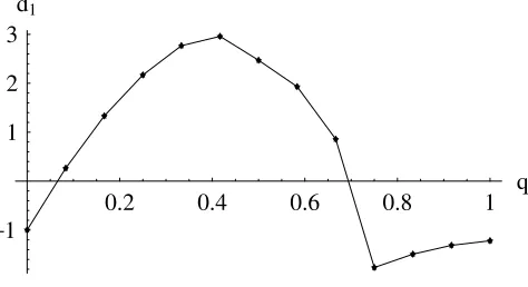
Let us first discuss the q-dependence of d1 for k1. The plot ofd1 is shown in Fig. 1. As discussed above the solution is stable forq0:75. One can see from the plot that the curve has a corner atq0:75. This is a general property for all values of k—the energy is not a
differ-entiable function ofqat the edge of the stability region. An interesting feature of the graph is that it crosses theq-axis twice, atq0:31andq0:72, i.e., for these values ofq
the coefficientd1 vanishes.5
The plot ofd1 fork2is shown in Fig. 2. In this case
the solution is stable forq0:4375. One can see that the curve crosses the q-axis only once in the stability region. To see that the energy is not differentiable in this case either, it is useful to plot d2, see Fig. 3. Even though, as
discussed above, the values ofd2 are not reliable, one can
clearly see thatd2is not smooth at the edge of the stability
region.
The plots ofd1fork4andk8are shown in Fig. 4
and 5. The solution is stable for q0:2344 and q
0:1211, respectively. The plots of d1 for all values of k
have similar shapes. In particular,d1 vanishes for at least one value qq? in the stability region. This value q?
depends onk, suggesting that one should not expect to find a simple dependence ofd1onkfor fixedq.
Indeed, while the leading correction in the classical energy E0 (2) scales with k as k2, there is no a priori
reason why the leading coefficient inE1 should also have
a simple dependence onk. The dependence of frequencies
!B
n and !Fr on k is such that it can be eliminated by rescaling!’s,, andn; rbyk[5] (see also Appendix A), but since this transformation involves a rescaling of sum-mation indices, the resultingE1(3) should, in general, be a nontrivial function of k. The dependence of d1 onk
be-comes nontrivial already for q 1
12 (see Fig. 6). (In the
formal case of q0 it is linear (d10;k 1 2k) as
TABLE I. Values ofd1q;k.
k1 k2 k4 k8
q0 0:50 1:00 2:00 4:00
q 1
12 0:34 0.26 7.9 74
q 2
12 0:20 1.33 16.1 1335 i
q 3
12 0:07 2.17 21:11:0 i 17213 i
q 4
12 0.03 2.77 24:02:7 i 20122 i
q 5
12 0.12 2.96 24:13:8 i 20641 i
q 6
12 0.17 2:470:77 i 22:38:0 i 19267 i
q 7
12 0.18 1:931:27 i 18:611:0 i 152101 i
q 8
12 0.13 0:861:73 i 8:718:1 i 78148 i
q 9
12 0:23 1:773:21 i 7:731:0 i 42275 i
q10
12 0:280:50 i 1:496:47 i 8:657:5 i 52470 i
q11
12 0:350:71 i 1:318:06 i 5:170:0 i 24575 i
q12
12 0:450:87 i 1:229:37 i 3:481:7 i 9673 i
4From numerical data in Table I we find, in agreement with the
analytic expression q1 11=2k2, that E1 becomes complex for q > q where 18=24< q<19=24 for k1, 5=12< q<6=12 for k2,2=12< q<3=12 for k 4, and1=12< q<2=12 for k8.
5Even though the coefficientd
Table I shows.) Sinced1121 ;1 0:34is negative and all
other values of d1121 ;k are positive, the k-dependence
cannot be given by a power functionkp. Rather the curve should be approximated by a polynomial of k. This ex-ample shows that in generald1 has a complicated depen-dence on k. As stated in the introduction, the one-loop gauge-theory computation of the corresponding coefficient
b1in (4) was carried out [15] only in the (unstable)q1
case with the resultb112k2. If that gauge-theory
predic-tionb1k2applies also to the stableq <1cases, then our
results would indicate a disagreement between the string-theory (d1) and the perturbative (1-loop) gauge-theory (b1) coefficients.
Let us now consider the special case ofq1, i.e.,J1
0,J2 J3 12Jin more detail. Here the frequencies can
be found in a simple analytic form [5] and the computation ofE1 becomes more explicit (see Appendix B). The cor-responding gauge-theory (4) result [15] written in the form (1) reads
J
11
2~k 211
J:::
. . .
: (20)
Here the leading-order term agrees [10] with the classical string energy (2); in order for the J~term in (20) to be in agreement with the one-loop string correction in (5) one should find that d1q1 1
2k
2. As already mentioned,
an apparent problem for checking this is that the q1
solution is unstable for any k1 [4,5]. In the simplest
case of k1 there is one imaginary bosonic frequency (for largerkthere are several unstable modes). As a result, the definition and interpretation of the 1-loop correction to the energy becomes nontrivial (formally, the 1-loop cor-rection then contains an imaginary part determining the rate of decay of the unstable state, see, e.g., [31]). In order to see if string-theory result may be put into an agreement with the gauge-theory result (20) we may try to use one of the following definitions of E1 (for definiteness, we shall consider the case ofk1):6
(i) computeE1as a sum over all frequencies as in (3) and (17), and omit the imaginary part; this amounts to ignoring the contribution of the one unstable bosonic mode with
n1.
(ii) analytically continue the value of the mass of the ‘‘tachyonic’’n1mode, i.e., include the contribution of its frequency toE1 with the modulus sign.7
In the case (i) we find by the numerical evaluation of the sum that d1 0:446. In the case (ii) we get instead d1 0:42 (the additional contribution of the modulus
of the frequency of the unstable n1 mode is
0.2 0.4 0.6 0.8 1 q
−1 1 2 3
[image:5.612.56.301.48.169.2]d1
FIG. 2. q-dependence ofd1fork2.
0.2
0.4
0.6
0.8
1
q
−
0.5
−
0.4
−
0.3
−
0.2
−
0.1
0.1
[image:5.612.315.565.52.178.2]d
1FIG. 1. q-dependence ofd1fork1.
0.2
0.4
0.6
0.8
1
q
−
40
−
30
−
20
−
10
d
2FIG. 3. q-dependence ofd2fork2.
6Formally, the unstable mode is not ‘‘seen’’ on the
gauge-theory side [10]. More precisely, an unstable mode of the 3-spin circular solution corresponds to the configuration when a Bethe root moves off the real axis [25,26]; this case does not corre-spond to a true eigenstate of the Hermitian Hamiltonian of the Heisenberg ferromagnet [9]. Still, this suggests that some ana-lytic continuation may apply. Related aspect of this problem is that the spin chain states found using the Bethe ansatz [10] are exact quantum states, while on the string-theory side we are considering semiclassical states dual to coherent states of the spin chain [19,21,32]. One can show (see also [23]) that the corresponding unstable mode is present also in the ‘‘Landau-Lifshits’’ sigma model which is the coherent state effective action following in the low-energy approximation from the Heisenberg spin chain Hamiltonian and which agrees [19] with a large spin limit of the string sigma model action.
7A possible way to support the second prescription is to view
theJ2J3,J10case as an analytic continuation of the stable solution with J2J3, J1>23J2. For this stable solution the spectrum of fluctuations (and thus E1) is real and matches with Bethe ansatzJ 1spectrum [11]. Then we may analyti-cally continue all relations in the angular momentum plane and try to define theJ1!0limit.
[image:5.612.61.298.574.703.2]*d1 3
p
2 0:866). This may look close to the 0.5 value in
(20), but our estimate of the numerical error is much smaller than 0.08, so we are inclined to conclude that there is a disagreement between the gauge-theory and string-theory values ford1, with a plausible explanation being the
same order-of-limits problem as in [27] (see also Sec. IV below).
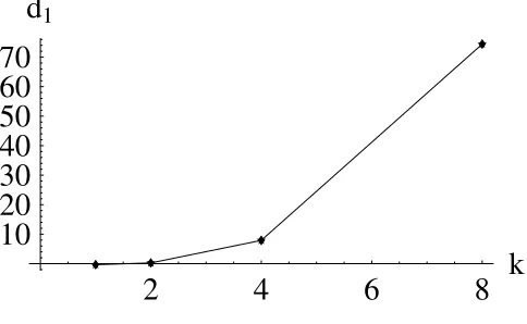
Finally, let us comment on thek-dependence ofd1in this q1case. Following the first prescription (i), i.e., keep-ing only the real part ofd1kwe get the plot in Fig. 7. It is
interesting to note that the curve can be well-approximated by the power function0:446kpwithp1:46.
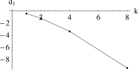
With the second prescription (ii), i.e., taking the sum of the real part and the imaginary part8ofd1we get the plot in Fig. 7. In this case it cannot be approximated by a power function. Comparing to (20) suggests again that there is a disagreement between the 1=J string-theory and gauge-theory results.
IV. CONCLUDING REMARKS
In this paper we have used numerical methods to analyze the leading 1-loop sigma model correction to the energy of the classical circular spinning string [4]. We have con-firmed the expected large Jexpansion of the energy, and studied the dependence of the first subleading coefficient
d1 in (1) on the two parameters —q2J2
J and ‘‘winding number’’k. Comparing our results with the known gauge-theory result [15] for the corresponding spin chain state (dual to unstable 2-spin circular string with q1), we have found a discrepancy not only in the numerical value but also in thek-dependence of the leading 1-loop coeffi-cientd1. Even though our computation is unambiguous and reliable only for the stable 3-spin string states with q
q<1, the differentk-dependence ofd1may be viewed as
an indication that there is a string/gauge-theory disagree-ment for the 1=J correction starting already at one-loop order on the gauge-theory side. We should add a
reserva-tion that it is still possible that the disagreement we find is due to the fact that the semiclassical quantization and its comparison to the gauge-theory side are not directly ap-plicable in the case of the unstable 2-spin solution, and there is still a chance that one may find a one-loop agree-ment for the stable 3-spin string states once one computes the corresponding1=Jgauge-theory corrections using the SU(3) Bethe ansatz of [11].
Assuming this1=Jdisagreement persists, it should have the same origin as the previously found mismatch between the string and gauge-theory results at 3-loop order inand the leading-order in J[18]. As was suggested in [18,27], the latter can be explained by adding ‘‘wrapping’’ contri-butions to the dilatation operator (and thus to the Bethe ansatz relations) on the gauge-theory side. For example, in theq1case one may use the function likeJ=1J which is one in the string-theory limit (J! 1with fixed
=J2 ~) but zero in the perturbative gauge-theory limit
to interpolate between the different3
J5results as follows:
J
2J 2 8J3
3 16J5
J3
1J3. . .:
This expression agrees with both the string (EpJ2
[4]) and the perturbative gauge-theory (pert J
2J 2
8J303::: [18]) results. The same idea may be applied to explain the discrepancy at order
J2:, for
ex-0.2
0.4
0.6
0.8
1
q
−
50
50
100
150
200
[image:6.612.322.563.50.185.2]d
1FIG. 5. q-dependence ofd1fork8.
0.2
0.4
0.6
0.8
1
q
−
5
5
10
15
20
[image:6.612.59.296.52.188.2]d
1FIG. 4. q-dependence ofd1fork4.
2
4
6
8
k
10
20
30
40
50
60
70
d
1FIG. 6. k-dependence ofd1 forq121. 8All unstable modes happen to have purely-imaginary
[image:6.612.320.562.558.707.2]ample, if we assume that the interpolation formula contains also a term
. . .
2J2
1a
J1
1J1
. . .;
then the gauge-theory limit result for the coefficientd1will
be1
2as in [15] while the string-theory limit will gived1 1
21a, explaining the apparent disagreement of our
result with that of [15].
A related observation is that this apparent1=J disagree-ment can be easily accommodated and thus explained within the generalized Bethe ansatz for quantum string spectrum recently proposed in [28]. To this end all one should do is to assume a definite largeLJexpansion of the functionscrg; L(g
8-2
p
) appearing in the Bethe ansatz of [28]. In particular, one can see that ifcrhave an expansion of the form crg; L ~r2L2r4~rL2r3,
then at order 1=L1=J there is a string/gauge-theory mismatch already for the coefficient of the one-loop (~) term. The Bethe ansatz of [28] also implies that if
there is a string/gauge-theory (dis)agreement for spinning string states at order 1=Jn then a similar (dis)agreement should exist also for the BMN states at order 1=Jn1. In
view of the above discussion, this suggests that for the BMN states the disagreement at order1=J2should start not
for 3-loop (3) terms as at1=Jorder but already for the
1-loop () terms.
ACKNOWLEDGMENTS
We are grateful to N. Beisert and K. Zarembo for useful discussions. Part of the work was done while S. F. visited SPHT/Saclay. He is grateful to I. Kostov and V. Schomerus for warm hospitality. The work of S. F. was supported in part by the 2004 Crouse Grant. The work of I. P. and A. T. was supported in part by the DOE Grant No. DE-FG02-91ER40690. I. P. is grateful to S. Mathur for his support and encouragement. A. T. acknowledges the hospitality of KITP at Santa Barbara during the completion of this work where his research was partly supported by the NSF under Grant No. PHY99-07949. A. T. is also supported by the INTAS Contract No. 03-51-6346 and a R. S. Wolfson Grant.
APPENDIX A: CLASSICAL SOLUTION AND QUADRATIC FLUCTUATIONS
The solution we discussed above was found in [4], and the characteristic equations for the quadratic fluctuations near it were obtained in [5]. Here we briefly review the derivation of the bosonic characteristic equation while in the fermionic case we only quote the final result referring to [5] for more details. The bosonic part of the string action in the conformal gauge is IpRdR2
-0 d2-
LAdSLS, where
LS 12@aXM@aXM12 XMXM1; (A1)
LAdS 122
PQ@
aYP@aYQ12~2
PQY
PYQ1: (A2) Here XM; M1;. . .;6 andYP; P0;. . .;5 are the em-bedding coordinates with a flat Euclidean metric forS5and with 2MN 1;1;1;1;1;1 for the AdS5 re-spectively. We consider the configuration where the string is located in the center of AdS5 while rotating inS5. The
AdS5 part of the solution is trivial (Y5iY0
eit; Y
1;. . .Y4 0), with the globalAdS5 time being set to t, while theS5 part is
X1iX2 q
p
coskeiw; X3iX4pqsinkeiw;
X5iX6p1qei
(A3)
with
w2 2k2; 2;
2 22k2q; qsin20:
(A4)
It was shown in [5] that the quadratic fluctuation
2
4
6
8
k
100
200
300
400
500
600
[image:7.612.57.299.51.180.2]d
1FIG. 8. k-dependence of d1 for q1 in the absolute value prescription.
2
4
6
8
k
−
8
−
6
−
4
−
2
d
1 [image:7.612.53.302.550.689.2]Lagrangian around this solution can be written as
L2 @X!s2 @X!s24 q
p
!
X5@X!6
4w p1qX!5@X!2X! 3@X!4
4k p1qX!5@X!3X! 2@X!4
: (A5)
The corresponding fluctuation spectrum is found by using
the following mode expansion
!
Xs X
1
n1
X8
h1
Asnhei!n;hn; (A6)
wherehlabels the different frequencies for a fixed value of
n. The determinant of the characteristic matrix is propor-tional to (here we set"!2
n)
B8" "4"38k24n220k2q82 "216k432k221648k2n2162n26n480k22q
80k4q36k2n2q96k4q2 "32k4n232k22n28k2n482n44n696k4n2q48k22n2q
12k2n4q96k4n2q2 16k4n48k2n6n816k4n4q4k2n6q: (A7)
The44S5-frequencies are obtained as!B n;S5
"
p
where"is one of the four roots ofB8 0. In addition, there are
44 AdS5 frequencies !n pn22: By following the analogous steps one can show [5] that the fermionic
characteristic frequencies!F
r are determined byF8" 0where
F8 2"4"38k21228r220k2q "212k428k221848k2r2282r212r452k4q
64k22q36k2r2q59k4q2 "8k620k4220k24868k4r28k22r2204r28k2r4
202r48r644k6q80k42q44k24q24k4r2q32k22r2q12k2r4q78k6q279k42q2
2k4r2q245k6q3 2k84k622k448k6r24k42r24k24r212k4r44k22r424r4
8k2r642r62r812k8q16k62q4k44q28k6r2q16k42r2q4k24r2q20k4r4q
4k2r6q27k8q221k62q22k44q230k6r2q211k42r2q211k4r4q227k8q39k62q3
9k6r2q381k
8q4
8 : (A8)
Unlike the bosonic case, the AdS5 and S5 parts are not
decoupled in the fermionic case. The eight fermionic fre-quencies are obtained by solving F8 0and taking!F
"
p
with double degeneracy.
When solving B8 0 one may set k1; then the k-dependence can be restored by the following rescaling,
!n!!n
k ; n!
n
k; !
k: (A9)
Similar rescaling can be done in the fermionic case [5]. Let us now consider the large -expansion of the bo-sonic frequencies to analyze the stability condition in that limit
!2
n!
h0
42 h1
4 : (A10)
Here
h0 n2
2k223q n2
2k
4n21q k2q9q8
q
: (A11)
The stability condition that follows from positivity ofh0is
[5]
qq; q1
1 1
2k 2
: (A12)
APPENDIX B:q1CASE:J10; J2J3
In the case ofq1the string is stretched around the big circle of S5 and rotates about its center of mass with two
equal angular momenta. Here the characteristic Eqs. (A7) and (A8) can be solved explicitly [5] and one finds that the bosonicS5 frequencies are (up to an overall sign change)
!B n
n2222k22q2k22n22 1=2
!B n
pn222k2p22k2: (B1)
This may be compared to theAdS5fluctuation frequencies !Bn
n22
p
!F r 12
2pr22k2p2k2p22k2
:
(B2) Using (B1) and (B2) we get the explicit form of (17) is
E1 1
"
1 p22k2p2k22
4
1
4 2k2
s !
X
N
n1
Sn; ;k
# ; (B3) where S
npn24k2242 s
2pn22k22
4pn224qn1=22k22
4
n1=22k22 q
(B4)
We have used that
n2222k22q2k22n221=2
n2222k22q2k22n221=2
2n2222k2 2npn24k21=2: (B5)
Note also that S!1!212k22n2
n n24k2
p
O1
3 and Sn!1!k
22k42
n3 On15, in agreement with (13).
One may be tempted to evaluate the sum in (B3) by converting it into an integral. This conversion is not pos-sible, however, due to singularities of the summand. To see this let us set k1 and follow the procedure of [5] to perform the large-expansion ofS for fixedn
x,
Sx Sx; ;1 !
!1
1
1x23=2 1
1671x
276x416x6 16x21x27=2
1
3. . .: (B6)
Note that the first term in the coefficient of 1
3 has a singularity atx0. This is an example of the singularities
that we discussed below (9). Even though we singled out the zero mode contribution in (17), it is this divergent behavior near x0 that is responsible for the failure of the conversion of the sum to an integral.
To estimate the accuracy of the numerical method that we used in Sec. III we approximately evaluate the tail of the sum in (B3). It is possible to convert the tail part of the sum in (B3), i.e.,1
P1
N1S, to an integral overxnsince it does not containx0or its neighborhood. Let us follow [5] and use that (we will not distinguish between N and
N1sinceN1)
1
X1
nN
SZ1
N
dxgx O 1
6
; (B7)
where
gx 2
15S
x1
6
5S
x 1
2
1
30Sx
2
15S
x 1
2
1
30S
x1
; (B8)
and Sx Sx; ;1. To evaluate the integral in (B7) consider the following large-xexpansion ofg,
g 1
2
3 1
x3
312 24
1
x4
353224 45
1
x5
5115264 86
1
x6
37721
2434106 167
1
x7:::: (B9)
Up to the order given in (B9) the integral yields
Z1
N
dxgx 1
2
11
N2 1 2
11
N3 3 16
2 3
2 5 4 3 N4 1 8
6 3
2 11 4 3
N5O 5
N6
: (B10)
For N400 00 and 50;100;200 we find that the correction is small compared to the numerically found value ofE1(which is of order105). However, the
correc-tion grows if we increasefor fixedN(e.g., consider
1000).
[1] D. Berenstein, J. M. Maldacena, and H. Nastase, J. High Energy Phys. 04 (2002) 013.
[2] S. S. Gubser, I. R. Klebanov, and A. M. Polyakov, Nucl. Phys.B636, 99 (2002).
[3] A. A. Tseytlin, hep-th/0311139; hep-th/0407218.
[4] S. Frolov and A. A. Tseytlin, Nucl. Phys.B668, 77 (2003). [5] S. Frolov and A. A. Tseytlin, J. High Energy Phys. 07
(2003) 016.
[6] S. Frolov and A. A. Tseytlin, Phys. Lett. B 570, 96 (2003).
[7] G. Arutyunov, S. Frolov, J. Russo, and A. A. Tseytlin, Nucl. Phys.B671, 3 (2003).
[8] G. Arutyunov, J. Russo, and A. A. Tseytlin, Phys. Rev. D
69, 086009 (2004).
[9] J. A. Minahan and K. Zarembo, J. High Energy Phys. 03 (2003) 013.
[10] N. Beisert, J. A. Minahan, M. Staudacher, and K. Zarembo, J. High Energy Phys. 09 (2003) 010.
[11] J. Engquist, J. A. Minahan, and K. Zarembo, J. High Energy Phys. 11 (2003) 063.
[12] S. Frolov and A. A. Tseytlin, J. High Energy Phys. 06 (2002) 007; A. A. Tseytlin, Int. J. Mod. Phys. A18, 981 (2003).
[13] A. Parnachev and A. V. Ryzhov, Int. J. Mod. Phys. A10, 066 (2002).
[14] C. G. Callan, H. K. Lee, T. McLoughlin, J. H. Schwarz, I. Swanson, and X. Wu, Nucl. Phys.B673, 3 (2003); C. G. Callan, T. McLoughlin, and I. Swanson, hep-th/0404007; hep-th/0405153.
[15] M. Lubcke and K. Zarembo, J. High Energy Phys. 05 (2004) 049.
[16] N. Beisert, S. Frolov, M. Staudacher, and A. A. Tseytlin, J. High Energy Phys. 10 (2003) 037.
[17] G. Arutyunov and M. Staudacher, J. High Energy Phys. 03 (2004) 004; hep-th/0403077.
[18] D. Serban and M. Staudacher, J. High Energy Phys. 06
(2004) 001.
[19] M. Kruczenski, Phys. Rev. Lett.93, 161602 (2004). [20] V. A. Kazakov, A. Marshakov, J. A. Minahan, and K.
Zarembo, J. High Energy Phys. 05 (2004) 024.
[21] M. Kruczenski, A. V. Ryzhov, and A. A. Tseytlin, Nucl. Phys.B692, 3 (2004).
[22] C. Kristjansen, Phys. Lett. B 586, 106 (2004); C. Kristjansen and T. Mansson, hep-th/0406176.
[23] R. Hernandez and E. Lopez, J. High Energy Phys. 04 (2004) 052.
[24] B. J. Stefanski, Jr. and A. A. Tseytlin, J. High Energy Phys. 05 (2004) 042.
[25] L. Freyhult, J. High Energy Phys. 06 (2004) 010. [26] J. A. Minahan, J. High Energy Phys. 10 (2004) 053. [27] N. Beisert, V. Dippel, and M. Staudacher, J. High Energy
Phys. 07 (2004) 075.
[28] G. Arutyunov, S. Frolov, and M. Staudacher, J. High Energy Phys. 10 (2004) 016.
[29] A. Mikhailov, J. High Energy Phys. 12, 058 (2003); hep-th/0402067.
[30] R. R. Metsaev and A. A. Tseytlin, Nucl. Phys.B533, 109 (1998).
[31] E. J. Weinberg and A. Q. Wu, Phys. Rev. D 36, 2474 (1987).