Optimization of Manufacturing Processes and of Systems Under the Conditions of Uncertainty

ISSN: 1816-949X

© Medwell Journals, 2020

Optimization of Manufacturing Processes and of Systems Under the

Conditions of Uncertainty

Alexander G. Madera

Scientific Research Institute for System Analysis, Russia Academy of Sciences,

Moscow, Russia

Abstract: This study is dedicated to optimization of manufacturing processes and manufacturing systems wherein interrelated activities are conducted in order to achieve the united common goal of converting the input flows of material, informational and financial resources into output ones valuable for the consumer. The process outcomes are a priori unknown and are determined by uncertain factors such as the future demand, risks and opportunities, the future states of the economy and finances, the market conjuncture, the prices of energy carriers and many others. In order to design the processes and process systems adequately, their mathematical optimization models must take into account the uncertainty of all the factors that exert influence on the course and outcomes of the processes in future. For this purpose, the study has devised a mathematical probabilistic optimization model of a process and process system with taking into account the uncertainty of the future values of the factors and the states of the (competitive, political, economic, financial, conjunctural, etc.) environment. A model in the form of an intervally stochastic random value with the arbitrary unimodal distribution of its values within their change interval has been accepted as the mathematical model of the factor uncertainty. The intervally stochastic model of the uncertainty is adequate for the real uncertainty and conforms to the agent’s psychology when making the decision and quantitatively estimating the uncertainties. The mathematical model devised by this study describes the processes conducted both in the separate manufacturing, ensuring, servicing links and in the process system in whole. To ensure the possibility of numerically determining the optimal parameter values for a process and process system, the probabilistic mathematical optimization model is reduced to a determinate mathematical optimization model, the solution of which can be effortlessly obtained by means of existing software intended for the solution of mathematical programming problems. The application of the devised mathematical models has been exemplified by optimization of a particular production process that includes ensuring and logistic processes, too. This study considers influence of the uncertain factors, such as investments into the process, future prices of the production factors and energy carriers, consumer’s demand, price of the end product, as well as future actualization of the possible opportunities and risks. It has been shown that the results of modelling and optimizing the processes under the uncertainty conditions are intervally stochastic and must be represented in the form of the intervals of their values depending on the probabilities of actualization of the risks and opportunities.

Key words: Manufacturing process, manufacturing system, process, uncertainty, mathematical model, optimization, interval, stochastic, criterion, constraints, opportunities, risks, prognostication INTRODUCTION

A process approach to management of various activities conducted in manufacturing process systems is actively developing both in scientific and in applied, practical aspects. The manufacturing process approach is directed at the management of processes which are aggregates of interrelated and interacting activities united by a single common goal and converting the input flows of material, informational and financial resources into output ones-an end product valuable for the consumer. At that, the process approach to management covers only those organizations and processes conducted therein that directly participate in converting the input flows into the output products. In order to conduct various activities

when processing the input resources into the end product, a process system is created which is a structured aggregate of links intended for various purposes (manufacturing, ensuring and servicing ones) in each of which the input (material, informational and financial) flows are purposefully converted into the output ones. Organizational units of any scale and form of ownership-from a workplace, site, production facility, department in an organization and a whole organization to enterprises, corporations and industries-may be the links in the process system.

system design stages can be performed only with a quantitative approach to the design which in turn, rests on mathematical models as well as methods for modelling and optimization. However, today processes and process systems, business processes in particular, whatever area of activity they belong to (manufacture, service, maintenance, ensuring, procurement, logistics) are modelled not quantitatively but on the contrary, qualitatively and descriptively in the form of verbal, textual, table, graphic and other descriptions, or notations, of the flows of works, resources, informational data, etc. (Vergidis et al., 2015; Brasseur et al., 2017). Existing literature dedicated to processes understands the modelling of processes as so-called regulation, documentation and accompanying document circulation and optimization as taking some measures to harmonize and partially improve the processes (Jeston and Nelis, 2013). However, fulfilment of any organizational prescriptions and taking measures are not actually optimization, since, the descriptive approach does not in principle ensure the optimal choice of the variants of acts, the optimal choice being scientifically understood as the achievement of the extremal value of an accepted quantitative criterion. At present, the design and modelling of business processes and process systems are usually substituted by their qualitative description and even if they contain quantitative methods, they are partial and specialized ad hoc (Brasseur et al., 2017).

Practically all the studies regard the manufacturing processes exclusively as determinate ones when all the factors that influence a process, as well as the environment, are fully and precisely known and determined. However, the real processes and process systems function under the conditions of uncertainty of the factors that determine the processes: risks and opportunities, future states of the economy and finances, market conjuncture and future prices of the resources and energy carriers, future demand for the new product for the sake of the creation of which a process is initiated, future financial position of the organizational units that participate in the process, their financial steadiness, etc. Uncertainty is an inherent attribute of the reality where an (individual or collective) agent acts and makes the decision. That is why the adequate mathematic modelling and optimization of the processes and process systems wherein they are conducted must take into account the uncertainties of the factors of the processes, process systems and environment (Raposo et al., 2000; Madera, 2014; 2015a; 2017).

This study is the development of quantitative methods for modelling and designing processes and process systems (Madera, 2015a, 2017). For this purpose, the study has devised probabilistic intervally stochastic mathematical optimization methods and models under the conditions of uncertainty of the factors of a process,

process system and (competitive, political, economic, financial, conjunctural, etc.) environment. The uncertain quantitative factors are modelled with an intervally stochastic model which is adequate for the real uncertainty and conforms to the agent’s psychology when making the decision and estimating the uncertainties. The obtained mathematical optimization models and methods may be used in order to make the quantitative design of process systems intended for various purposes when conducting diverse activities in the spheres of manufacture, ensuring, procurement, maintenance, rendering services, logistics and supply chains. (The work has been performed within the project 0065-2019-0001 implemented under the government order for fundamental scientific research GP 14).

MATERIALS AND METHODS

The structural and mathematical models of manufacturing processes and process links: The structural model of a process system is an aggregate of interacting links (organizational units) in each of which diverse activities are conducted in order to pursue a united common purpose that consists in making the end output product valuable for the consumer. The inputs of the process links receive the flows of resources (production factors) which are converted into (end or intermediate) products at the link’s outputs. The production factors are divided into exogenous, endogenous and energenous ones (conditioned by the expenditures of various kinds of energy) which form the sets X, Y and Z, namely:

The set X of the exogenous factors {x} = {x1, x2, ..., xn}0X, id est the resources bought up in the external-relative to the process-environment.

The set Y of the endogenous factors {y} = {y₁, y₂, …, yk}0Y, id est the intermediate products manufactured within the process in the previous links (or processes) and coming to the inputs of the following links of the process.

z3(2) z3(1) x1 z1(2)

z1(1) x1

1

x2 x2

3 y2 5

x4

x5 y3 4 y1

x3 2

z4(2) _z

4(1) z2(1)

z2(2)

z5(1)

z5(2) _z

6(2)

z6(1)

y4 6 y

In general, all the kinds of the resources-endogenous ones as well as exogenous resources and energenous factors belonging to them-are fed to the input of each process link. In the sets X and Y, the numeration of the exogenous and endogenous flows is independent and consecutive throughout the whole structure of the process system.

We will mark out the following processes and their respective links (Madera, 2015a; 2017): the manufacturing or main, processes add value and cost to the end or intermediate product equal to the product manufacture expenditures. In the manufacturing link, the material factors of production that are fed to the link input are converted into the product at its output (intermediate product, semi-finished product, work in progress, end product) and at the same time, the cost of the input factors is converted into the link output product cost conditioned by the expenditures incurred in the link during the manufacture.

The ensuring processes add cost but not valueand in principle are ballast ones. They change neither the amount nor the quality of the products and production factors regarding which the ensuring works are done but they require expending the production factors (energy carriers and auxiliary means of production) which adds cost to the product. The amounts of the production factors and intermediate products at the input and output of the ensuring link remain unchanged, except for the expended energy carriers and live labor. The ensuring kinds of works include: Loading, unloading, sorting, delivery of the production factors and/or intermediate products to the workplace, storage and maintenance, execution of the accompanying documents, etc.

The servicing processes or services, add value for the consumer and are accompanied by adding end product cost equal to the expenses for the servicing works for which the exogenous and energenous factors are expended. In the servicing link, just as in the ensuring

one, there is no quantitative change in the amount of the product over which the servicing works are performed. The servicing works include: packing, sorting, marking, imparting marketable style, delivery directly to the consumer, etc.

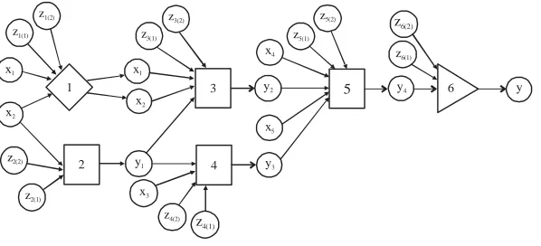
In the structural model of a process and its corresponding process system, the flows of the exogenous, endogenous and energenous factors of production are designated by circles inside which the amounts of the (x-exogenous, y-endogenous, z-energenous) factors are specified; the entry of the resources and/or products is designated by arrows; the manufacturing links are designated by rectangles; the ensuring ones are designated by rhombi and the servicing ones are marked by triangles.

The structural model of a process system given as an example in Fig. 1 contains an ensuring link 1, four manufacturing links 2, 3, 4, 5 and a servicing link 6. The exogenous production factors amounting to x₁, x₂, x₃, x₄, x5 come from the environment (bought up outside the process) to the inputs of the process links, as well as the endogenous products amounting to y1, y2, y3, y4, y5 manufactured within the process in links 2, 3, 4 and the energenous production factors zi(1) (energy carriers) and zi(2) (live labor), i = 1, 2,...,6. A flow amounting to y4 is the manufactured end product which is the ultimate goal of the whole process and a flow amounting to y(= y4) is the end product over which the servicing works are then done in link 6. The amounts of the flows of the resources and products at the input and output of ensuring link 1 and servicing link 6 do not change anyhow when the respective ensuring or servicing works are done over them, except for the energenous production factors which are always expended in all the activities and all the links. Let us consider the mathematical models of the process links (Madera, 2015a; 2017).

Manufacturing link: The mathematical model of a manufacturing link i, to the input whereof the (ordered) sets of the exogenous XidX, endogenous YidY and energenous ZidZ production factors {xi1, xi2,...,xin}0Xi, {yi1, yi2,...,yik}0Yi, {zi1, zi2}0Zi are fed is a multifactor Manufacturing Function (MF) (Fare, 1988) equal in natural units to yl = fi(xi1, xi2,…,xin; yi1, yi2, …, yik, zi2) where, yl0Y is the amount of the product manufactured in the link i.

Simultaneously with physically converting the production factors that come to the link input into the product at its output, the cost of the input flow of the factors increases by the value of the expenses that accompany the manufacturing works in the link for processing them into the product (hereinafter the expenses are understood as the so called average expenses, or the product amount unit expenses).

Let us mark the costs of the amount (price) units of the exogenous, endogenous and energenous production factors that come to the input of the manufacturing link i as {p1, p2,...,pn}, {q1, q2,...,qk} and {r1, r2}, respectively. Then at the output of the manufacturing link, the total cost Cman _{of the product will be equal to the sum of the costs of} the exogenous



k

j j j 1q y



production factors at the link input as well as the cost of the energy carriers r1z1 and the cost of the live labor r2z2 the expenditures of which are the expenses proper for the manufacturing works done when processing the inputs into the outputs, namely:

n k

man

j j j j 1 1 2 2

j 1 j 1

C 





Ensuring and servicing links: Unlike the manufacturing links where the production factors from the link inputs are converted into qualitatively new products at the outputs, the ensuring links do works for servicing and ensuring the manufacturing works and the servicing ones do works for the service treatment of the ready-made product manufactured in the process system.

In the course of the ensuring and servicing activities, the production factors are expended only for the respective maintaining and servicing works and by no means for qualitative and quantitative changes in the products treated in these links. The ensuring processes deal with the intermediate, unfinished products, production factors and semi-finished products; the servicing ones deal with the ready-made products already manufactured in the process system. The manufacture-ensuring works do not add any value to the product. On the contrary, the servicing works add value, since, they are connected with rendering services to the clients for which they are ready to pay. According to the aforesaid, the mathematical models of the ensuring and servicing links will have the following peculiarities:

In the ensuring link, at the link’s input and output, the amounts of the exogenous and endogenous flows of the production factors are equal to each other and do not change throughout the ensuring operations performed in the link, except for, perhaps, artifacts such as stealing, damage, etc., at that, the energenous factors are expended in any link and during any works.

In the servicing link, the exogenous and energenous production factors that come to the input are expended and processed in the course of the servicing works over the ready-made product that comes to the input of the servicing link and the endogenous factors of production do not come to the input of the servicing link. The amount of the ready-made product that comes to the input of the servicing link does not change after the servicing works done over it; however, value and cost are added.

In the ensuring link, according to its characteristic, the mathematical model of conversion of the amounts of the production factors will be written in the form of the following correlations xi = xi and yj = yj, i = 1, 2,…, n, j = 1, 2,…, k.

In the servicing link, according to its characteristic and taking into account that the product amount y (= yout) remains unchanged from the input to the output of the servicing link, the mathematical model that describes conversion of the production factors amounting to x1, x2, ..., xn; z1, z2 at the input of the servicing link into the product amounting to y at its output will be written as y = f (x1, x2,...,xn; z1, z2; y). Let us consider the cost-value conversions performed in the ensuring and servicing links.

All the (exogenous, endogenous and energenous) production factors come to the ensuring link and the operations performed in it do not lead to a change in the amounts and qualitative characteristics of the exogenous and endogenous factors, except for the energenous factors (energy carriers and human labor) expended in full. That is why the total cost of the production factors in the ensuring link Censur _{will be determined by the same} expression that is for the manufacturing link Cman _(see above).

In addition to the exogenous and energenous factors of production, the end product manufactured as a result of the process comes to the input of the servicing link and there are no endogenous factors. Consequently, the total cost of the activities conducted in the servicing link Cserv consists of the costs of the endogenous and energenous factors at the input of the servicing link as well as the cost of the end output product that enters the servicing link from the output of the whole process; the total cost amounts to y (= yout), namely:

n

serv proc

j j 1 1 2 2

j 1

where, Cproc _{is the total cost of the end product at the} output of the whole process as related to the unit of its amount.

The total cost Cproc _{of all the production factors and} works done in the whole process system will be determined by the expression:

(1)

proc

j j i 1 1 i 2 2

i {proc} j

i

{p x } {r z} {r z}



 

 _   _

 

 

C

where, the sums are done both for all the links of the process system (the index and for all the production factors (the index j = 1, 2, ...) in each separate process link (manufacturing and ensuring one). Since, the costs of the production factors include the costs of (expenses for) the works done in the process links, the total summed cost Cproc _{will equal the total cost of the end product made in} the process system (as related to the unit of its amount). Mathematical optimization model of a manufactoring process system under the conditions of uncertainty of the future states of the process factors and environment: There are differences in principle between the manufacturing, ensuring and servicing links. Indeed, the manufacturing processes are orientated towards the future demand for and supply of the products made as a result of them; the ensuring ones are aimed at the performance of ensuring works over the already manufactured (ready-made, work-in-progress) products in the amounts determined by the requirements of the manufacturing process proper; the servicing ones are aimed at rendering the ordered services in the amounts determined by contracts between the operators of the manufacturing and servicing processes (outsourcing is also possible) or between the process operator and the client. The ensuring works are additional non-manufacturing expenses that are included in the cost of the end product and do not add any value to it, that is why the operator of the manufacturing process is always willing to decrease the ensuring works. The servicing works require additional expenses, too but add value to the ready-made product and the consumer is ready to pay for the value. That is why approaches to the design of the manufacturing, ensuring and servicing links and processes substantially differ from each other.

To ensure a high level of adequacy, mathematical models and methods for optimization of the processes and process systems must include the uncertainty of the future outcomes and consequences of the activities conducted in the process system, the uncertainty being conditioned by the uncertainties of the future states of the economy, finances, market conjuncture, prices of energy carriers, competitive environment, investments, economic and financial positions of the organizations that form the process system, etc. The uncertainty of the future

outcomes and consequences of the activities conducted in a process system manifests itself in the form of uncertainty of future actualization of two different in principle, events, namely (Madera, 2014): Risks (losses, insufficient profit, failures, misfortunes) and opportunities (high profits, good luck, achievement of the planned outcomes). As researches into decision-making psychology (Kozielecki, 1981; Raposo et al., 2000; Kahneman et al., 2001; Madera, 2014; 2015a) show, under the conditions of uncertainty, when choosing the decision that is the best for them, an agent orientates themself, first of all, towards the maximization of their opportunities, id est future good luck, profits, success and only after that they consider the chosen decisions from the position of the possible risks which express the future misfortunes, failures, damage and possible obstacles which at that, they try to minimize. The fact that the success image prevails over the failure image in the agent’s mind motivates them to conduct certain activities, despite the difficulties that may actualize on their way. Because man is not endowed with the capability to prognosticate the future unambiguously and precisely, to give accurate estimates and make fully reliable judgements, the agent is aware-when making the decision that, since, the actualization of both the future success and the possible future failure is unpredictable, then when conducting the activities, they should prefer the future success and orientate themself towards the achievement of the set goal as the motivational engine for conducting the activities (Kahneman et al., 2001). The agent also understands that orientation only towards the possible risks as it is accepted in most of the existing studies can lead only to refusal of any creative efforts and activities in general, since, an activity without risks is just doing nothing.

Under the conditions of uncertainty, the mathematical optimization model of a process and the process system wherein the process takes place contains numerical factors (parameters) the values of which actualize only in the future. Such uncertain factors include the future demand for the manufactured product, prices of the production factors, investments into the process, values of the risks and opportunities and many other things that are always of an uncertain nature. That is why in order to ensure adequacy of the mathematical model that describes a process under the conditions of uncertainty, it is necessary to have at one’s disposal a mathematical model that describes the uncertainties of the quantitative factors.

problem being solved, the different researchers introduce additional assumptions regarding the character of uncertainty of the interval factors. For example, studies suppose only the knowledge of the boundaries of the uncertain factor’s change interval, without introducing any assumptions as to the function of the factor’s distribution within the interval (Alefeld and Herzberger, 1983). Studies (Kibzun and Kan, 1996; Kahneman et al., 2001; Liu, 2009; Madera, 2016; 2017) construe the uncertain factors within their intervals as random values that conform to certain probability distributions. Being a priori unknown, the probability distributions can be both unimodal with an expressed expected value around which (symmetrically or asymmetrically) group the values of an uncertain factor and uniform ones (Feller, 1968; Kibzun and Kan, 1996; Kahneman et al., 2001; Madera, 2015b; 2016; 2017). The plausibility of prognostication of the interval boundary values is measured by an inductive probabilistic measure (Carnap, 1971; Madera, 2014).

This study has accepted an intervally stochastic model of an uncertain factor, namely, the uncertain factor ξ is an interval random value [ξ(ω)], ω0Ω (ω are elementary events from the sample space Ω), that complies with the unimodal function of distribution with the density p(ξ),ξ0[ξ_{_}, 'ξ] and p(ξ) = 0, ξó [ξ_{_}, 'ξ] in the interval [ξ_{_}, 'ξ] (ξ_{_} and 'ξ are the lower and upper boundaries of the interval). Let us note that no additional assumptions regarding the particular kind of the function of distribution of the intervally stochastic value [ξ(ω)]0 [ξ_{_}, 'ξ] are done.

Probabilistic intervally stochastic optimization mathematical model of a process system: Let us build the mathematical optimization model of a process and process system under the conditions of uncertainty having formed the target function and constraints for this purpose.

According to the aforesaid, a relevant and valid optimization criterion for the process has to reflect the possible future actualization of both opportunities and risks and making the best decision under the conditions of uncertainty suggests that the opportunities must be maximized and on the contrary, the risks must be minimized. The maximized complex Opportunities-Risks (Op&R) criterion satisfies these conditions (Madera, 2014; 2015a; 2017):

(2)

Op R

Op&R =  Op- R max

where, Op&R are the generalized opportunities and risks prognosticated by the agent that are relevant to the activity under consideration; θOp, θR0[0,1] are the coefficients of the relative importance of the opportunities and risks and θ_Op+θ_R = 1.

The values of the generalized opportunity Op and generalized risk R are proportional to their quantitative M_op, M_R and probabilistic P_op, P_R measures (Madera, 2014); the generalized values are determined as the products Op = Mop@POpи R = MR@PR. The quantitative measure expresses the desired value of the profit, if the opportunity conditions actualize and an insufficient or negative profit, if the risk conditions actualize. The probabilistic measure is the probability of future actualization of the opportunity or risk conditions-events relevant to the process goal-profit (Madera, 2014). Since, the generalized opportunity and generalized risk reflect the profit from the process, their quantitative measures M_Op and M_R must be equal to the profit values Pr_Op and PrR, if the opportunity and risk conditions of the process realize, the conditions actualizing with the probabilities POp and PR in the future. That is why in the Opportunities-Risks criterion Op&R, the total values of the generalized opportunity and generalized risk will equal Op = PrOp@POp and R = PrR@PR, respectively.

According to the conception of the generalized opportunities Op and risks R, some of these events will actualize for sure-that is why the events consisting in the occurrence of either the generalized opportunities Op or the generalized risks R form the complete group of the events for which the equality POp+PR = 1 is true.

The total generalized opportunities Op and risks R contain all the events relevant to the process under consideration that can actualize in the future reality in the form of L opportunities and K risks included in the set of the risks and opportunities M which form the complete group of the events. Let us note that the set M can contain the following events:

Opportunities: Which include the achievement of the desired profit level, low prices of the production factors and energy carriers, advantageous currency exchange rate, increased demand for the new product, favorable competitive environment, rather a large amount of the investments, stable financial position of the organizational units involved in the process.

Risks: Which include zero, negative (direct losses) or insufficient profit that does not cover the expenses, high prices of the production factors end energy carriers, currency weakening, low or no demand for the new product, competitor’s launching successful substitutes, reduction of the consumer’s effective demand level, unfavorable market conjuncture.

Because the process profit values are uncertain intervally stochastic [PrOp(ω)] and [PrR(ω)] under the opportunity PrOp and risk PrR conditions, the optimization criterion will also be intervally stochastic, namely:

(3)

Op Op Op R R

In Eq. 3, under the opportunity [PrOp(ω)] and risk [PrR(ω)]

conditions, the values of the uncertain intervally stochastic profits have taking into account Eq. 1, the following appearance:

(4)

Op y,out Op out

j Op j i 1 Op 1 i 2 Op 2 i

i {proc} j

[Pr (ω)] [s (ω)] y

{[p (ω)] x } {[r (ω)] z } {[r (ω)] z }



  

 

    

 

 

(5)

R y,out R out

j R j i 1 R 1 i 2 R 2 i

i {proc} j

[Pr (ω)] [s (ω)] y

{[p (ω)] x } {[r (ω)] z } {[r (ω)] z }



 

 

    

 



 

where, y_out is the amount of the manufactured end product at the output of the whole process which is the sought value and equal to the manufacturing function of the last link in the process system under the prognosticated opportunity and risk conditions (Op/R); [Sy,out(ω)]Op/R is the intervally stochastic value of the selling price of the process output end product manufactured in an amount of under the prognosticated opportunity and risks conditions (Op/R); [Pj(ω)]Op/R,i, [r1(ω)]Op/R,i and [r2(ω)]Op/R,i are the intervally stochastic prices of the production factors bought up under the prognosticated opportunity and risk conditions (Op/R). All the input intervally stochastic factors are independent.

The constraints of the optimization model have to express the following conditions: The conditions of receiving profit not less than the permissible value both if the opportunity (PrOp

perm_{) conditions actualize, id est} {[Pr_Op(ω)]$Pr_Opperm_{} and if the risk (Pr}

R

perm_{) conditions} realize, id est {|[Pr_R(ω)]|$Pr_Rperm_}.

The budgetary constraints both under the opportunity {[COp

perm_{(ω)]#[I(ω)]}

Op} and risk {[CR

perm_{(ω)]#[I(ω)]} R} conditions. Which actualize jointly with the occurrence of one out of two independent events: either an opportunity (Op) or a risk R which form the complete group.

Here C_Opperm _{is the total cost of all the production} factors that come to the process system link inputs including the expenses for doing works in the process system under the opportunity/risk (Op/R) conditions (refer to (1)). It has also been taken into account that the profit from the process, the amounts of the investments and the total cost of the process are uncertain intervally stochastic under the opportunity/risk conditions.

Being supplemented with the condition of non-negativity of the model’s optimization variables {x} and {z}, the complete probabilistic model of a process and process system will take the final appearance:

(6)

{x},{z} Op Op Op R R R

P{max ( [Pr ( )] P -   |[Pr ( )]| P )}   

perm perm

Op Op Op R R R

P P{{[Pr ( )] Pr }|Op}+P P{{|[Pr ( )]| Pr }|R} 

(7)

proc proc

Op Op Op R R R

P P{{[C ( )] [I( )] }|Op}+P   P{{[C ( )] [I( )} }|R   

(8) (9)

{x}, {z} 0

if the conditions P_Op+P_R = 1 and θ_Op+θ_R = 1 are satisfied. The mathematical model 6-9 determines the optimal values of the production factor amounts {x},{z} at which the probability (Eq. 6) of the event that consists in the opportunities-risks criterion’s achieving its maximum, as well as the probabilities of the events that consist in fulfilling the constraints both on the desired profit amount (Eq. 7) and the process budget (Eq. 8) will not be less than the preset values of the threshold probabilities

α, β, γ.

We are reminding that the probabilistic measures or the probabilities of actualization of all the uncertain events P{@}, just as the particular threshold values of the probabilities α, β, γ. have a subjective character and are assigned by an (individual or collective) agent proceeding from their own perceptions and understanding of the conducted activities and achievement of the desired results, as well as from available historical and modern statistical data relevant to the process under consideration. In the mathematical model 6-9 the intervally stochastic values of the profits [Pr(ω)], process cost [Cproc_{(ω)] and} investments [I(ω)] change in their respective interval_{[Pr, Pr],[C}proc_{, C}proc_{]and[I, I].}

z1(1) z1(2)

x1 x2

x3

Warehouse

Manufacture Manufacture z2(1)

z2(2)

x1 x2

2

x3

z3(1) z3(2)

y1 3

y2 y y2 = out 1

Having reduced probabilistic inequalities 6-8 of the probabilistic mathematical model to their equivalent determinate form (Liu, 2009), we have obtained the final determinate mathematical model of such a process system or its determinate equivalent:

(10)

-1 {x},{z}

max {E{[Op&R( )]}+   ( ) {[Op&R( )]}}













 

 









perm perm

Op Op R R 1

Op R

R Op

Pr E [Pr (ω)] Pr E | [Pr ω ] |

P P Ψ 1 β

σ | [Pr ω ] |

σ[Pr (ω)]



 

    

(11)

(12)



 



















 

proc

Op Op

Op proc

Op Op

proc

R R 1

R proc

R R

E [C (ω)] E [I(ω)] P

σ[C (ω)] [I(ω)]

E [C (ω)] E [I(ω)]

P Θ γ

σ[C (ω)] [I(ω)]



 

 

 

 





(13)

{x},{z} 0

where, Φ, Ψ, Θ are the distributions of the probabilities of the intervally stochastic values of the [Op and R(ω)] criterion, the profits [PrOp] and [PrR(ω)] as well as the total costs of the process [C_Opproc_{] and [C}

R

proc_{] if the} opportunity/risk conditions (Op/R) actualize; E{[Op and R(ω)]}, E{[PrOp(ω)]}, E{[PrR(ω)]} and σ

2_{{[Op and} R(ω)]}, σ2_{[Pr

Op(ω)]} are the mathematical expectations (E{×}) and variances (σ2_{{×}) of the intervally} stochastic values of the [Op and R(ω)] criterion and profits [PrOp(ω)], [PrR(ω)] determined according to the expressions:

Op Op Op R R R

E{[Op&R( )]} =   E{[Pr ( )]} P -   |E{[Pr ( )]}| [P 

 

Op Op Op R R R

σ{[Op&R ω ] = θ σ{[Pr (ω)]} P + θ σ {[Pr (ω)]} P

The intervally stochastic values of the profits [PrOp(ω)] and [PrR(ω)] as well as their statistical measures E{[Op&R(ω)]}, E{[PrOp(ω)]}, E{[PrR(ω)} and σ

2_{[Op &R(ω)], σ2_{[Pr

Op(ω)]}, σ 2_{[Pr

R(ω)]} being determined on the basis of expressions (Eq. 4 and 5).

The determinate mathematical optimization model 10-13 determines the optimal non-negative amounts of the production factors {x}, {z} that impart the maximal value to the target function (Eq. 10) and at the same time, satisfy constraints (Eq. 11 and 12). The determinate model 10-13 does not contain uncertainties, probabilistic conditions-constraints and belongs to the class of common problems of non-linear programming. It is rather difficult to solve non-linear optimization models of this class and they have no effective methods yet to guarantee finding the global optimal solution. If the global extremum of a non-linear optimization model exists, the complexity of determining it is conditioned by the presence of the set of local extrema with an a priori unknown quantity which does not guarantee the successful choice of the global extremum, even if one exhaustively searches it from among all the obtained local extrema, their quantity being unknown. In some cases, if the feasible region is convex and the target function is convex, concave or square one in a non-linear programming problem, the global extremum always exists is the sole one and can be successfully found (Taha, 2017). A particular appearance of the probabilistic optimization mathematical model 6-9 and its determinate equivalent 10-13 is established when considering a real process and the process system where it is conducted.

RESULTS AND DISCUSSION

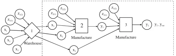
Modelling and optimizing a manufactoring process at practice: A production process system (Fig. 2) is intended for production of some end product and includes an ensuring link 1 (input warehouse) wherein logistic processes are performed and a manufacturing system (links 2 and 3). The ensuring warehouse link 1 does not participate directly in the manufacturing process and taking into account that there is no subject for optimization in it (above in detail), link 1 has not been included in the manufacturing subsystem (outlined with a dashed line, Fig. 2). Let us note that the logistic processes that are performed over the production factors and accompany the manufacturing processes within the manufacturing system (sorting, loading, unloading,

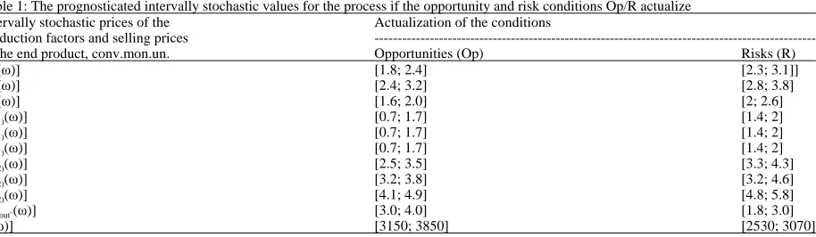
Table 1: The prognosticated intervally stochastic values for the process if the opportunity and risk conditions Op/R actualize

Intervally stochastic prices of the Actualization of the conditions

production factors and selling prices

---of the end product, conv.mon.un. Opportunities (Op) Risks (R)

[p1(ω)] [1.8; 2.4] [2.3; 3.1]]

[p2(ω)] [2.4; 3.2] [2.8; 3.8]

[p3(ω)] [1.6; 2.0] [2; 2.6]

[r1(1)(ω)] [0.7; 1.7] [1.4; 2]

[r2(1)(ω)] [0.7; 1.7] [1.4; 2]

[r3(1)(ω)] [0.7; 1.7] [1.4; 2]

[r1(2)(ω)] [2.5; 3.5] [3.3; 4.3]

[r2(2)(ω)] [3.2; 3.8] [3.2; 4.6]

[r3(2)(ω)] [4.1; 4.9] [4.8; 5.8]

[Sy,out`(ω)] [3.0; 4.0] [1.8; 3.0]

[I(ω)] [3150; 3850] [2530; 3070]

feeding to the workplace, etc.) are by their conceptual meaning, ensuring ones and this is why they are considered jointly with the manufacturing process. At the same time, the logistic processes that are conducted outside the process (delivery of the production factors, warehouse activities, loading-unloading, consolidation, etc.) and do not belong to its operator (for example, outsourcing) are not included in the manufacturing system of the process.

To ensure the manufacturing process, exogenous x1, x2, x3 and energenous z2(1), z3(1) (energy carriers), z2(2), z₃₍₂₎, (live labor) production factors are expended and energenous factors z1(1), z1(2) are expended for the warehouse activities over the production factors x1, x2, x3 (ensuring link (1) The amounts of the production factors that participate in the manufacturing process are subject to optimization in order to determine both the optimal amount of the process output product y₂ = y_out to be manufactured for yielding the maximal profit and the amounts of the exogenous x₁, x₂, x₃ and energenous z₂₍₁₎, z3(1), z2(2), z3(2) factors to be purchased at the prices p1, p2, p3 and r3(1), r1(2), r3(2), respectively existing at the moment. In addition to the exogenous and energenous production factors, the intermediate (endogenous) product manufactured within the process in manufacturing link 2, is used in the manufacture of the process output end product (output of manufacturing link 3); the intermediate (endogenous) product’s amount y1 is also subject to optimization.

After having been purchased, the exogenous factors x₁, x₂, x₃ of production go to the warehouse (link 1), wherefrom the factors x1, x2, jointly with the energenous factors z₂₍₁₎ and z₂₍₂₎ are fed to manufacturing link 2 where they are processed into an intermediate product amounting to y₁. The intermediate product amounting to together with the energenous z3(1), z3(2) factors and the exogenous one x₃, which comes from the warehouse (link 1) are then fed to the input of manufacturing link 3 wherein they are processed into the process output end product amounting to y2 = yout.

The purchase prices of the production factors [pop(ω)], [rOp(ω)], [pR(ω)], [rR(ω)], the selling price of the ready-made product [Sy,out,Op], [Sy,out,R] and the amounts of the investments into the designed process [I(ω)]Op, [I(ω)]R,

under the conditions of a priori unknown actualization of the opportunity or risk conditions are uncertain intervally stochastic values (Table 1).

The prognosticated probability values are POp = 0.65 and P_R = 0.35, α = 0.6, β = 0.65, γ = 0.65 and the parameters set by the process agent equal θOp = 0.65,

θR = 0.32, the permissible threshold profit values amount to Pr_Opperm _{= 7500 and Pr}

R

perm _{= 4500 conv.mon.un. In} view of the fact that the quantity of the members in the sums of the intervally stochastic values that are included in the expressions of determinate equivalent 10-13 is more than three, the probability distributions Φ, Ψ, Θ of these sums conform to the normal abridged law of distribution within the boundaries of the domain intervals. The probabilistic model of the process is described by system 6-9 and its determinate equivalent is described by system 10-13 with the intervally stochastic values refer to 4, 5:

Proc

Op/R y,out (Op/R) out Op/R

[Pr ( )] = [S ( )] y -[C ( )]

 

 





3 proc

Op/R i Op/R i i(1) Op/R i(1) i(2) Op/R i(2)

i 1

[C (ω)] [p (ω)] x [r ω] z [r ω] z







and statistical measures: Mathematical expectations:

 

Op/R y, out Op

proc

out Op/

/R R

{[Pr (ω)]} {[S (ω)]} y E{[C (ω)]}

E E

 

 

 

xi Z

Z

3 proc

Op/R[ i i(1) Op/R i 1

i 1

i( 2) Op/R i(2

R

)

Op/

{[C (ω)]} (E{[p (ω)]} +E{[r ]}

E{[r ]}



  





E

Root-mean-square deviations:

2 2 2 proc

Op/R y,out (Op/R ) out Op/R

σ{[Pr (ω)]} σ{[s (ω)]} y σ{[C (ω)]}

 





1/2 3

2 2 2 2

i Op/R i i 1 Op/R i(1)

proc

i 1 Op/R

2 2

i(2) Op/R i(2)

σ{[p (ω)]} x σ{[r ω]} z

σ{[C (ω)]}

σ{[r ω]} z

( )

( )



 _{ }

 

  

 

 

80000

70000

60000 50000

40000 30000

20000 10000

0

In

te

rv

al p

ro

fit f

ro

m

th

e p

ro

c

ess

0 0.25 0.5 0.75

Probability of risk conditions

Fig. 3: Intervally stochastic value of the process profit depending on the probability of actualization of the risk conditions for the future outcomes of the manufacturing process

The manufacturing function of the whole manufacturing process (Fig. 2) equals:





0.5

0.65 0.55 0.4 0.5 0.7 0.5 0.7

2 3 1 2 2(1) 2(2) 3 1 3(2)

y = 0.01x 0.05x x z z z z

The optimal solution (found by means of software intended for solving non-linear programming problems) is: x1 = 129.04, x2 = 72.79, x3 = 362.25, z(2(1) = 186.52, z2(2) = 106.81, z(3(1) = 360.70, z3(2) = 159.09 conv.un., yout = 11564.6 conv.un. The statistical measures of the profit under the opportunity conditions equal: The mathematical expectation E{[PrOp(ω)]} = 37603 and the root-mean-square deviation σ{[PrOp(ω)]} conv.mon.un.

Due to the intervally stochastic character of the input uncertain factors of the process, the process profit is also intervally stochastic and as the computations show, changes within an interval limited by its upper and lower boundaries (Fig. 3). At that, the relative span of the interval profit (received as a result of the process) changes within the range of 31-37%, thus, demonstrating that the fluctuations in the intervally stochastic profit can be rather significant under the real uncertainty conditions. The character of the obtained dependence (Fig. 3) shows that the higher the probability of actualization of the risk conditions, unfavorable for conducting the process and obtaining the desired result, the smaller the process profit and its span (width of the change interval).

CONCLUSION

This study proposes a conception, models and methods for mathematically modelling and optimizing processes and process systems under the conditions of uncertainty of the future states of the economy and finances as well as of the process-determining factors such as the future demand, prices of the production factors, selling price of the end product, amount of the investments, actualization of the possible opportunities (favorable future events) and risks (unfavorable future events), market conjuncture, etc. The structural model of a process system includes manufacturing, ensuring and servicing links. An intervally stochastic probabilistic and its equivalent determinate optimization mathematical models of the processes and process systems have been devised. The said models use a complex opportunities-risks criterion as the optimization criterion which maximizes the opportunities, simultaneously minimizes the risks for the processes and to the most adequate degree reflects the future uncertainty to make the process decisions. The mathematical models and methods elaborated by this study permit the mathematical modelling and optimization of the processes and process systems without being limited by complexity of the process system structure.

The researches done in this article show that the process estimation criterion the profit being the one is an interval value which changes within an interval limited by its upper and lower boundaries determined by the character of the activity that is conducted in the process system, the accepted technologies, intensity of implementing the innovations and accuracy of prognosticating the uncertainties. It has been shown that the span of the fluctuations of the interval profit from the process can change within rather wide limits and sometimes achieve 40%. Due to this, the output resulting final data for the socioeconomic processes must be represented in the form of interval values and not precisely in a single definite value, as it is often presented in existing literature on the modelling of economic processes. It is not adequate for the reality to neglect the interval character of the modelling results, the final profits from the processes in particular.

REFERENCES

Alefeld, G. and J. Herzberger, 1983. Introduction to Interval Computations. 1st Edn., Academic Press, New York, USA., ISBN-13: 978-0120498208, Pages: 352.

Carnap, R., 1971. Logical Foundations of Probability. 2nd Edn., University of Chicago Press, Chicago, USA., Pages: 613.

Fare, R., 1988. Fundaments of Production Theory. 1st Edn., Springer, Berlin, Germany, ISBN:978-3-540-50030-8, Pages: 163.

Feller, W., 1968. An Introduction to Probability Theory and Its Applications. 3rd Edition/Vol. 1, Wiley, New York, USA., ISBN:9780471257080, Pages: 528. Jeston, J. and J. Nelis, 2013. Business Process Management. 3rd Edn., Routledge, New York, USA., ISBN-13:978-0415641760, Pages: 688.

Kahneman, D., P. Slovic and A. Tversky, 2001. Judgment under Uncertainty: Heuristics and Biases. Cambridge University Press, Cambridge, USA, Pages: 555. Kibzun, A.I. and Y.S. Kan, 1996. Stochastic

Programming Problems with Probability and Quantile Functions. Wiley, Chichester, New Hampshire, ISBN:9780471958154, Pages: 316.

Kozielecki, J., 1981. Psychological Decision Theory. Kluwer Academic Publishers, Boston, Massachusetts, USA., Pages: 403.

Liu, B., 2009. Theory and Practice of Uncertain Programming. 2nd Edn., Springer, Berlin, Germany, ISBN:978-3-540-89483-4, Pages: 198.

Madera, A.G., 2014. [Risks and Opportunities: Uncertainty, Forecasting and Evaluation]. Krasand, Russia, ISBN:978-5-396-00570-9, Pages: 448 (In Russian).

Madera, A.G., 2015b. Interval uncertainty of estimates and judgments of subject in decision making in multi-criteria problems. Intl. J. Anal. Hierarchy Process, 7: 337-348.

Madera, A.G., 2015a. [Mathematical modeling and optimization of business processes based on the comprehensive criterion of chances-risks (In Russian)]. Russ. J. Manage., 26: 51-68.

Madera, A.G., 2016. Estimating the probability of forecasted events. Intl. J. Accounting Econ. Stud., 4: 76-80.

Madera, A.G., 2017. Modeling and optimization of business processes and process systems under conditions of uncertainty. Bus. Inf., 4: 74-82. Raposo, A.B., L.P. Magalhaes and I.L.M. Ricarte, 2000.

Petri nets based coordination mechanisms for multi-workflow environments. Comput. Syst. Sci. Eng., 15: 315-326.

Taha, H.A., 2017. Operations Research: An Introduction. 10th Edn., Pearson Education, New Jersey, USA., ISBN-13:978-0134444017, Pages: 848.