warwick.ac.uk/lib-publications
Original citation:
Duong, Manh Hong and Han, The Anh. (2016) Analysis of the expected density of internal
equilibria in random evolutionary multi-player multi-strategy games. Journal of
Mathematical Biology .
Permanent WRAP URL:
http://wrap.warwick.ac.uk/80462
Copyright and reuse:
The Warwick Research Archive Portal (WRAP) makes this work by researchers of the
University of Warwick available open access under the following conditions. Copyright ©
and all moral rights to the version of the paper presented here belong to the individual
author(s) and/or other copyright owners. To the extent reasonable and practicable the
material made available in WRAP has been checked for eligibility before being made
available.
Copies of full items can be used for personal research or study, educational, or not-for profit
purposes without prior permission or charge. Provided that the authors, title and full
bibliographic details are credited, a hyperlink and/or URL is given for the original metadata
page and the content is not changed in any way.
Publisher’s statement:
“The final publication is available at Springer via
http://dx.doi.org/10.1007/s00285-016-1010-8
."
A note on versions:
The version presented here may differ from the published version or, version of record, if
you wish to cite this item you are advised to consult the publisher’s version. Please see the
‘permanent WRAP url’ above for details on accessing the published version and note that
access may require a subscription.
(will be inserted by the editor)
Analysis of the expected density of internal
equilibria in random evolutionary multi-player
multi-strategy games
Manh Hong Duong · The Anh Han
Received: date / Accepted: date
Abstract In this paper, we study the distribution and behaviour of internal equilibria in ad-playern-strategy random evolutionary game where the game payoff matrix is generated from normal distributions. The study of this paper reveals and exploits interesting connections between evolutionary game theory and random polynomial theory. The main contributions of the paper are some qualitative and quantitative results on the expected density, fn,d, and the
expected number,E(n, d), of (stable) internal equilibria. Firstly, we show that in multi-player two-strategy games, they behave asymptotically as√d−1 asd
is sufficiently large. Secondly, we prove that they are monotone functions ofd. We also make a conjecture for games with more than two strategies. Thirdly, we provide numerical simulations for our analytical results and to support the conjecture. As consequences of our analysis, some qualitative and quantitative results on the distribution of zeros of a random Bernstein polynomial are also obtained.
Keywords Random evolutionary games · Internal equilibria · Random polynomials·Multi-player games
1 Introduction
1.1 Motivation
Evolutionary game theory (EGT) has been proven to be a suitable mathemat-ical framework to model biologmathemat-ical and social evolution whenever the success
Manh Hong Duong
Mathematics Institute, University of Warwick, UK. E-mail: [email protected]
The Anh Han
of an individual depends on the presence or absence of other strategies [34,
27,39]. EGT was introduced in 1973 by Smith and Price [35] as an applica-tion of classical game theory to biological contexts, and has since then been widely and successfully applied to various fields, not only biology itself, but also ecology, population genetics, and computational and social sciences [34,
4,27,39,10,41,23,17]. In these contexts, the payoff obtained from game inter-actions is translated into reproductive fitness or social success [27,39]. Those strategies that achieve higher fitness or are more successful, on average, are favored by natural selection, thereby increase in their frequency. Equilibrium points of such a dynamical system are the compositions of strategy frequencies where all the strategies have the same average fitness. Biologically, they pre-dict the co-existence of different types in a population and the maintenance of polymorphism.
As in classical game theory with the dominant concept of Nash equilibrium [37,36], the analysis of equilibrium points in random evolutionary games is of great importance because it allows one to describe various generic properties, such as the overall complexity of interactions and the average behaviours, in a dynamical system. Understanding properties of equilibrium points in a concrete system is important, but what if the system itself is not fixed or undefined? Analysis of random games is insightful for such scenarios. To this end, it is ambitious and desirable to answer the following general questions:
How do the equilibrium points distribute? How do they behave when the number of players and strategies change?
in-ternal equilibrium points for the general case, a lower and upper bounds the multi-player two-strategy random games, and a close-form formula for the two-player multi-strategy games.
In this paper, we address the aforementioned questions, i.e., of analysing distributions and behaviours of the internal equilibria of a random evolutionary game, in an average manner. More specifically, we first analyse the expected density of internal equilibrium points,fn,d(t), i.e. the expected number of such
equilibrium points per unit length at pointt, in ad-playern-strategy random evolutionary game where the game payoff matrix is generated from a normal distribution (for short, normal evolutionary games). Here the parameter t= (ti)ni=1−1, withti=xxi
n, denotes the ratio of frequency of strategyi∈ {1,· · · , n−
1} to that of strategy n, respectively (more details in Section 2). In such a random game, we then analyse the expected number of internal equilibria,
E(n, d), and, as a result, characterize the expected number of internal stable
equilibria, SE(n, d). We obtain both quantitative (asymptotic formula) and qualitative (monotone properties) results offn,d and E(n, d), as functions of
the ratios,t, the number of players,d, and that of strategies,n.
To obtain these results, we develop further the connection between EGT and random polynomial theory explored in [14], and more importantly, estab-lish appealing (previously unexplored) connections to the well-known classes of polynomials, the Bernstein polynomials and Legendre polynomials. In con-trast to the direct approach used in [16,22], our approach avoids sampling and solving a system of multivariate polynomial equations, thereby enabling us to study games with large numbers of players and/or strategies.
We now summarise the main results of the present paper.
1.2 Main results
The main analytical results of the present paper can be summarized into three categories: asymptotic behaviour of the density function and the expected number of (stable) equilibria, a connection between the density function with the Legendre polynomials, and monotonic behaviour of the density function. In addition, we provide numerical results and illustration for the general games when both the numbers of players and strategies are large.
To precisely describe our main results, we introduce the following notation regarding asymptotic behaviour of two given functions uand v: [0,+∞) →
[0,+∞)
u.v ⇔ there exists a positive constantC such that for allk∈[0,+∞)
u(k)≤Cv(k),
u∼v ⇔ it holds that u.v and v.u.
fn,d(t), besides t, is also analyzed as a function ofn and d. We will
explic-itly state which parameter(s) is being varied whenever necessary to avoid the confusion.
The main results of the present paper are the following. As described above,
fn,d(t) denotes the expected number of internal equilibrium points per unit
length at point t, in a d-player n-strategy random evolutionary game where the game payoff matrix is generated from a normal distribution; E(n, d) the expected number of internal equilibria; andSE(n, d) the expected number of internal stable equilibria. The formal definitions of these three functions are given in Section2.
(1) In Theorem1, we prove the following asymptotic behaviour off2,d(t) for
allt >0:f2,d(t)∼
√
d−1. We also prove thatf2,d(t) is always bounded
from above and limd→∞f2d,d−(1t) = 0.
(2) In Theorem 2, we prove a novel upper bound for the expected number of multi-player two-strategy random games, E(2, d) . √d−1 ln(d−1) and obtain its limiting behaviour: lim
d→∞
lnE(2,d) ln(d−1) =
1
2. This upper bound
is sharper than the one obtained in [14, Theorem 2], which is, E(2, d). (d−1)34. These results lead to two important corollaries. First, we obtain
a sharper limit for the expected number of stable equilibria, SE(2, d).
1 2
√
d−1 ln(d−1), and the corresponding limit, lim
d→∞
lnSE(2,d) ln(d−1) =
1 2, see
Corollary 1. The second corollary, Corollary 2, is mathematically signif-icant, in which we obtain lower and upper estimates and a limiting be-haviour of the expected real zeros of a random Bernstein polynomial. (3) In Theorem3, we establish an expression off2,d(t) in terms of the Legendre
polynomial and its derivative.
(4) In Theorem4, we expressf2,d(t) in terms of the Legendre polynomials of
two consecutive order.
(5) In Theorem 5, we prove that f2,d(t)
d is a decreasing function ofdfor any
givent >0. Consequently, E(2d,d) and SE(2d,d) are decreasing functions of
d.
(6) In Proposition 2, we provide a condition for f2,d(t) being an increasing
function ofdfor any givent >0. We conjecture that this condition holds true and support it by numerical simulation.
(7) In Theorem 6, we provide an upper bound for fn,2(t). We also make a
conjecture forfn,d(t) andE(n, d) in the general case (n, d≥3).
(8) We offer numerical illustration for our main results in Section4.2. The density functionfn,d(t) provides insightful information on the distribution
of the internal equilibria: integrating fn,d(t) over any interval produces the
expected number of real equilibria on that interval. In particular, the expected number of internal equilibriaE(n, d) is obtained by integratingfn,d(t) over the
positive half of the space. Theorem 5 and Proposition 2, which are deduced from Theorems 3 and 4, are qualitative statements, which tell us how the expected number of internal equilibria per unit lengthf2,d in ad-player
quantifies its behaviour showing thatf2,d is approximately (up to a constant
factor) equal to√d−1. The functionh(d) :=√d−1, as seen in Theorem1, certainly satisfies the properties thath(d) increases but h(dd) decreases. Thus, it strengthens Theorem 5 and further support Conjecture 1. Theorem 2 is also a quantitative statement which provides asymptotically estimate for the expected number of internal (stable) equilibria.
Furthermore, it is important to note that the expected number of real zeros of a random polynomial has been extensively studied, dated back since 1932 with Block and P´olya seminal paper [6] (see, for instance, [15] for a nice exposition and [45,38] for the most recent progresses). Therefore, our results, in Theorems3,4and2, provide important, novel insights within the theory of random polynomials, but also reveal its intriguing connections and applications to the EGT.
1.3 Organisation of the paper
The rest of the paper is structured as follows. In Section2, we recall relevant details on EGT and random polynomial theory, to the extent we need here. Section3presents full analysis of the expected density function and the expect number of internal equilibria of a multi-player two-strategy game. The results on asymptotic behaviour and on connection to Legendre polynomials and its applications are given in Sections 3.1 and 3.2, respectively. In Section4, we provide analytical results for the two-player multi-strategy game and numerical simulations for the general case. Therein we also make a conjecture about an asymptotic formula for the density and the expected number of internal equilibria in the general case. In Section 5, we sum up and provide future perspectives. Finally, some detailed proofs are presented in the appendix.
2 Preliminaries: replicator dynamics and random polynomials
This section describes some relevant details of the EGT and random polyno-mial theory, to the extent we need here. Both are classical but the idea of using the latter to study the former has only been pointed out in our recent paper [14].
2.1 Replicator dynamics
The classical approach to evolutionary games is replicator dynamics [46,50,
27,44,39], describing that whenever a strategy has a fitness larger than the average fitness of the population, it is expected to spread. Formally, let us consider an infinitely large population withnstrategies, numerated from 1 to
n. They have frequenciesxi, 1≤i≤n, respectively, satisfying that 0≤xi≤1
and Pn
randomly selected groups ofdparticipants, that is, they play and obtain their fitness from d-player games. We consider here symmetrical games (e.g. the public goods games and their generalizations [24,26,43,40,21]) in which the order of the participants is irrelevant. Letαi0
i1,...,id−1 be the payoff of the focal
player, wherei0 (1≤i0≤n) is the strategy of the focal player, and ik (with
1 ≤ ik ≤n and 1 ≤ k ≤d−1) be the strategy of the player in position k.
These payoffs form a (d−1)-dimensional payoff matrix [16], which satisfies (because of the game symmetry)
αi0
i1,...,id−1 =α
i0
i0
1,...,i0d−1, (1)
whenever{i0
1. . . , i0d−1}is a permutation of{i1. . . , id−1}. This means that only
the fraction of each strategy in the game matters.
The equilibrium points of the system are given by the points (x1, . . . , xn)
satisfying the condition that the fitness of all strategies are the same, which can be simplified to the following system ofn−1 polynomials of degreed−1 [14]
X
0≤k1,...,kn≤d−1, n
P
i=1
ki=d−1
βik1,...,kn−1
d−1
k1, ..., kn
n
Y
i=1
xki
i = 0 fori= 1, . . . , n−1, (2)
where βi
k1,...,kn−1 := α
i
k1,...,kn−α
n
k1,...,kn, and
d−1
k1, . . . , kn
= (dn−1)! Q
k=1
ki!
are the multinomial coefficients. Assuming that all the payoff entries have the same probability distribution, then allβi
k1,...,kn−1, i= 1, . . . , n−1, have symmetric
distributions, i.e. with mean 0 [22].
We focus on internal equilibrium points [16,22,14], i.e. 0< xi <1 for all
1≤i≤n−1. Hence, by using the transformationti=xxni, with 0< ti<+∞
and 1≤i≤n−1, dividing the left hand side of the above equation byxd−1
n
we obtain the following equation in terms of (t1, . . . , tn−1) that is equivalent
to (2)
X
0≤k1,...,kn−1≤d−1, n−1
P
i=1
ki≤d−1
βki1,...,kn−1
d−1
k1, ..., kn
n−1
Y
i=1
tki
i = 0 fori= 1, . . . , n−1.
(3) Hence, finding an internal equilibria in a generaln-strategy d-player random evolutionary game is equivalent to find a solution (y1, . . . , yn−1)∈R+n−1 of
2.2 Random polynomial theory Suppose that allβki
1,...,kn−1 are Gaussian distributions with mean 0 and
vari-ance 1, then for eachi (1 ≤i≤n−1), Ai =
βki
1,...,kn−1
d−1
k1, ..., kn
is a multivariate normal random vector with mean zero and covariance matrixC
given by
C= diag
d−1
k1, ..., kn
2!
0≤ki≤d−1, n−1
P
i=1
ki≤d−1
. (4)
The density functionfn,d and the expected numberE(n, d) of equilibria can
be computed explicitly. The lemma below is a direct consequence of [15, Theorem 7.1] (see also [14, Lemma 1]). For a clarity of notation, we use bold font to denote an element in high-dimensional Euclidean space such as t= (t1, . . . , tn−1)∈Rn−1.
Lemma 1 Assume that{Ai}
1≤i≤n−1 are independent normal random vectors
with mean zero and covariance matrix C as in (4). The expected density of
real zeros of Eq. (3)at a point t= (t1, . . . , tn−1)is given by
fn,d(t) =π−
n
2Γ
n
2
(detL(t))12, (5)
whereΓ denotes the Gamma function andL(t)the matrix with entries
Lij(t) =
∂2
∂xiyj
(logv(x)TCv(y))
y=x=t,
with
v(x)TCv(y) = X
0≤k1,...,kn−1≤d−1, n−1
P
i=1
ki≤d−1
d−1
k1, . . . , kn
2 n
Y
i=1
xki
i y ki
i . (6)
As a consequence, the expected number of internal equilibria in a d-player
n-strategy random game is determined by
E(n, d) =
Z
Rn+−1
fn,d(t)dt. (7)
3 Multi-player two-strategy games
We provide mathematical analysis of the expected density functionf2,d(t) and
3.1 Asymptotic behaviour of the density and the expected number of equilibria
In the case of multi-player two-strategy games (n= 2), the system of polyno-mial equations in (2) becomes a univariate polynomial equation
d−1
X
k=0
βk
d−1
k
yk(1−y)d−1−k= 0, (8)
where y is the fraction of strategy 1 (i.e., 1−y is that of strategy 2) and
βk is the payoff to strategy 1 minus that to strategy 2 obtained in ad-player
interaction withkother participants using strategy 1. It is worth noticing that
bk,d:=
d−1
k
yk(1−y)d−1−k, k= 0, . . . , d−1, (9)
is the Bernstein basis polynomials of degreed−1 [42,32]. Therefore, the left-hand side of (8) is a random Bernstein polynomial of degree d−1. As a by-product of our analysis, see Theorem2, we will later obtain an asymptotic formula of the expected real zeros of a random Bernstein polynomial.
Lett=1−yy (t∈R+), Eq. (8) is simplified to
d−1
X
k=0
βk
d−1
k
tk = 0. (10)
The expected density of real zeros of this equation at a point t isf2,d(t).
For simplicity of notation, from now on we write fd(t) instead of f2,d(t). We
recall some properties of the density function fd(t) from [14, Proposition 1]
that will be used in the sequel.
Proposition 1 ([14]) The following properties hold
1) fd(0) =d−π1, fd(1) = d2−π1√21d−3.
2) fd(t) =21π
1
tG
0(t)12 , where
G(t) =t
d dtMd(t)
Md(t)
=td
dtlogMd(t) with Md(t) =
d−1
X
k=0
d−1
k
2
t2k.
(11)
3) fd(t)has an alternative representation
(2πfd(t))2= d−1
X
i=1
4ri
(t2+r
i)2
, (12)
whereri>0 satisfies that Md(t) = d−1
Q
i=1
(t2+r
i).
5) fd 1t
=t2f(t).
6) E(2, d) =R0∞fd(t)dt= 2
R1
0 fd(t)dt.
Example 1 Below are some examples offd(t), withd= 2,3 and 4
f2(t) =
1
π
1
1 +t2, f3(t) =
2
π √
1 +t2+t4
1 + 4t2+t4, f4(t) =
3
π √
1 + 4t2+ 10t4+ 4t6+t8
1 + 9t2+ 9t4+t6 .
We recall thatt=1−yy, whereyis the fraction of strategy 1. We can write the density in terms ofy using the change of variable formula as follows.
fd(t)dt=fd
y
1−y
1
(1−y)2dy.
Definegd(y) to be the density on the right-hand side of the above expression,
i.e.,
gd(y) :=fd
y
1−y
1
(1−y)2. (13)
The following lemma is an interesting property of the density function gd,
which explains the symmetry of the strategies (swapping the index labels con-verts an equilibrium at y to one at 1−y). Numerical simulations in Section
4.2further illustrate this property (see Figure6).
Lemma 2 The functiony7→gd(y)is symmetric about the line y=12, i.e.,
gd(y) =gd(1−y).
Proof We have
gd(1−y) =fd
1−y
y
1
y2 =fd
y
1−y
y2
(1−y)2
1
y2 =fd
y
1−y
1
(1−y)2 =gd(y),
where we have used the fifth property in Proposition1 to obtain the second equality above.
The following theorem provides an upper bound and asymptotic behaviour forfd(t) and its scaling with respect to d.
Theorem 1 (Asymptotic behaviour of the density function) The fol-lowing statement holds
fd(t)≤min
√d−1
2π t , d−1
π
for t≥0. (14)
As a consequence, for any givent >0
fd(t)
d−1 ≤
1
π, dlim→∞ fd(t)
d−1 = 0, (15)
and furthermore
fd(t)∼
√
Proof It follows from the first and the fourth properties in Proposition1 that
fd(t)≤fd(0) =
d−1
π . (17)
On the other hand, according to the third property in Proposition1, we have
(2πfd(t))2= d−1
X
i=1
4ri
(t2+r
i)2
.
Since (t2+ri)2≥4rit2, it follows that for anyt6= 0
(2πfd(t))2≤ d−1
X
i=1
1
t2 =
d−1
t2 ,
which is equivalent tofd(t)≤
√
d−1
2π t . Hence, the upper bound of fd(t) in (14)
holds.
The upper bound and limit in (15) are obvious consequences of (14). It remains to prove the asymptotic behaviour offd(t) as a function ofd. Using
(14) and the fourth property in Proposition1, it follows that, for 0< t≤1
d−1 2π
1
√
2d−3 =fd(1)≤fd(t)≤
√ d−1 2π t ,
and fort≥1 1
t2
d−1 2π
1
√
2d−3 = 1
t2fd(1)≤
1
t2fd
1
t
=fd(t)≤fd(1) =
d−1 2π
1
√
2d−3. From these estimate, we deduce thatfd(t)∼
√
d−1 for anyt >0. We numerically illustrate Theorem1in Section4.2, see Figures1. Theorem 2 (Asymptotic behaviour of E(2, d))It holds that
√
d−1.E(2, d).√d−1 ln(d−1). (18)
Furthermore, we obtain the following asymptotic formula forE(2, d)
lim
d→∞
lnE(2, d) ln(d−1) =
1
2. (19)
Proof The lower bound was derived previously in [14, Theorem 2]. For the sake of completeness, we provide it again here. Using the sixth and the fourth properties in Proposition 1, we haveE(2, d) = 2R1
0 fd(t)dt ≥2
R1
0 f(1)dt=
2f(1) = d−1
π√2d−3. Therefore,
√
d−1.E(2, d).
The underlying idea of the proof for the upper bound is to split the integral range in the formula of E(2, d) into two intervals. The first one is from 0 to
α, for some α∈(0,1); we then estimate fd(t) in this interval byfd(0). The
second one is fromαto 1, which is estimated using the upper bound offd(t)
given in (14). The value ofαwill then be optimized.
E(2, d) = 2
Z 1
0
fd(t)dt= 2
Z α
0
fd(t)dt+
Z 1
α
fd(t)dt
≤2
αfd(0) +
√ d−1
2π
Z 1
α
1
t dt
= 1
π h
2(d−1)α−√d−1 lnαi. (20) Let h(α) be the expression inside the square brackets in the right-hand side of (20). To obtain the optimal (i.e. smallest) upper bound, we minimizeh(α) with respect toα. The optimal value ofαsatisfies the following equation
d
dαh(α) = 2(d−1)− √
d−1
α = 0,
which leads toα= 2√1
d−1. Substituting this value into (20), we obtain
E(2, d)≤ √
d−1
π
1 + ln 2 +1
2ln(d−1)
.
It follows thatE(2, d).√d−1 ln(d−1), which is (18). We now prove (19). By taking logarithm in (18), we obtain
1
2ln(d−1).lnE(2, d). 1
2ln(d−1) + ln ln(d−1). Therefore
1 2 .
lnE(2, d) ln(d−1) .
1 2 +
ln ln(d−1)
ln(d−1) . (21) Since lim
d→∞
ln ln(d−1)
ln(d−1) = 0, we achieve (19).
Theorem2 has two interesting implications about the expected number of stable equilibrium points in a random game and that of real zeros of a random Bernstein polynomial.
Corollary 1 The expected number of stable equilibrium points in a random game withd players and two strategies, SE(2, d), satisfies
√ d−1
2 .SE(2, d). 1 2
√
and furthermore, satisfies the following limiting behaviour
lim
d→∞
lnSE(2, d) ln(d−1) =
1
2. (23)
Proof From [22, Theorem 3], it is known that an equilibrium in a random game
with two strategies and an arbitrary number of players, is stable with prob-ability 1/2. Thus, SE(2, d) = E(22,d). Hence, the corollary is clearly followed from Theorem2.
Corollary 2 The expected number of real zeros,EB, of a random Bernstein polynomial
B(x) =
d−1
X
k=0
βk
d−1
k
xk(1−x)d−1−k,
whereβk are independent standard normal distributions, satisfies
√
d−1.EB. √
d−1 ln(d−1), lim
d→∞
lnEB
ln(d−1) = 1
2. (24)
Proof As mentioned beneath (8), solving B(x) = 0 is equivalent to solving
Eq. (10). It follows that fd(t) is the expected density of real zeros of B(x).
Therefore,EB given by
EB=
Z ∞
−∞
fd(t)dt= 2
Z ∞
0
fd(t)dt= 2E(2, d). (25)
Note that the second equality in (25) holds because fd(t) is even in t due
to (12). The asymptotic behaviour (24) ofEB is then followed directly from Theorem2.
Remark 1 The study of distribution and expected number of real zeros of a
random polynomial is an active research field with a long history dating back to 1932 with Block and P´olya [6], see for instance [15] for a nice exposition and [45,38] for the most recent results and discussions. Consider a random polynomial of the type
Pd(z) = d−1
X
i=0
ciξizi. (26)
The most well-known classes of polynomials studied extensively in the litera-ture are: flat polynomials or Weyl polynomials forci:= 1i!, elliptic polynomials
(EP) or binomial polynomials for ci :=
s
d−1
i
and Kac polynomials for
ci := 1. We emphasize the difference between the polynomial studied in this
paper, i.e. the right-hand side of Eq. (10), with the elliptic polynomial: in our case ci =
d−1
i
elliptic polynomial. In the former case, v(x)TCv(y) = Pd−1
i=1
d−1
i
xiyi =
(1 +xy)d−1, and as a result the density function and the expected number of
real zeros have closed formula, see [15]
fEP(t) =
√ d−1
π(1 +t2), EEP =
√ d−1.
Our case is more challenging, because of the square in the coefficients,
v(x)TCv(y) =Pd−1
i=1
d−1
i
2
xiyi is no longer a generating function.
Nev-ertheless, Theorem 2 shows that E(2, d) still has interesting asymptotic be-haviour as in (18) and (19).
3.2 Connections to Legendre polynomials and other qualitative properties In this section, we first establish a connection between the expected density functionfdand the well-known Legendre polynomials. Then using the
connec-tion and known properties of Legendre polynomials, we prove some qualitative properties of fd and the expected number of equilibria. The main results of
this section can be summarised as follows.
(i) Theorem3and Theorem4derive an expression for the expected density
fd in terms of the Legendre polynomials.
(ii) Theorem5 shows that fd(t)
d−1 is an increasing function ofdfor any given
t >0.
(iii) Corollary4 proves that Ed(2−,d1) and SEd−(21,d) are decreasing functions ofd. Technically, keys to these theorems are Lemma3 that connects the Legendre polynomials Pd to Md+1 in (11), and Lemma 4 showing a reverse Turan’s
inequality. These lemmas are interesting on their own.
3.2.1 Legendre polynomials
We recall some relevant details on Legendre polynomials. Legendre polynomi-als, denoted byPd(x), are solutions to Legendre’s differential equation
d dx
(1−x2) d
dxPd(x)
+d(d+ 1)Pd(x) = 0, (27)
with initial data P0(x) = 1, P1(x) = x. The following are some important
properties of the Legendre polynomials that will be used in the sequel. (1) Explicit representation
Pd(x) =
1 2d
d
X
i=0
d
i
2
(2) Recursive relation
(d+ 1)Pd+1(x) = (2d+ 1)xPd(x)−dPd−1(x). (29)
(3) First derivative relation
x2−1
d P
0
d(x) =xPd(x)−Pd−1(x). (30)
Example 2 The first few Legendre polynomials are
P0(x) = 1, P1(x) =x, P2(x) =
1 2(3x
2−1), P 3(x) =
1 2(5x
3−3x),
P4(x) =
1 8(35x
4−30x2+ 3).
The Legendre polynomials were first introduced in 1782 by A. M. Legen-dre as the coefficients in the expansion of the Newtonian potential [33]. This expansion gives the gravitational potential associated to a point mass or the Coulomb potential associated to a point charge. In the course of time, Legendre polynomials have been widely used in Physics and Engineering. For instance, they occur when one solves Laplace’s equation (and related partial differential equations) in spherical coordinates [5].
Our approach reveals an appealing, and previously unexplored relationship between Legendre polynomials and evolutionary game theory. We explore this relationship and its applications in the next sections.
3.2.2 From Legendre polynomials to evolutionary games
The starting point of our analysis is the following relation between the poly-nomialMd+1(t) in (11) and the Legendre polynomialPd.
Lemma 3 It holds that
Md+1(t) = (1−t2)dPd
1 +t2
1−t2
. (31)
Proof See Appendix6.1.
Note that traditionally in the Legendre polynomials, the arguments are in [−1,1]. In this paper, however, the arguments are not in this interval since
1+t
2
1−t2
≥ 1. Legendre polynomials with arguments greater than unity have
been used in the literature, for instance in [13, Chapter 2]. We now estab-lish a connection between the density fd(t) with the Legendre polynomials.
According to the second property in Proposition1, we have
fd+1(t) =
1 2π
"
1
t
tM
0
d+1(t)
Md+1(t)
0#
1 2
, (32)
where0denotes the derivative with respect tot. Using this formula and Lemma
3, we obtain the following expression of fd+1(t) in terms of Pd(t) and its
Theorem 3 (Expression of the density in terms of the Legrendre polynomial and its derivative) The following formula holds
(2π fd+1(t))2=
4d2
(1−t2)2 −
16t2
(1−t2)4
P0
d
Pd
21 +t2
1−t2
(33)
Proof See Appendix6.2.
Corollary 3 As a direct consequence of (33), we obtain the following bound forf2,d(t)which is interesting on its own.
fd(t)≤
1
π d−1
1−t2. (34)
In comparison with the estimate (14) obtained in Theorem 1, this inequality
is weaker for t >0since it is of order O(d−1). However, it does not blow up ast approaches 0.
We provide another expression offd+1(t) in terms of two consecutive Legendre
polynomials Pd−1 and Pd. In comparison with (33), this formula avoids the
computations of derivative of the Legendre polynomialPd.
Theorem 4 (Expression of the density function in terms of two Leg-endre polynomials) It holds that
(2πfd+1(t))2=
4d2
(1−t2)2 −
d2
t2
1 +t2
1−t2 −
Pd−1
Pd
1 +t2
1−t2
2
. (35)
Proof See Appendix6.3
3.2.3 Monotonicity of the densities
Theorem4is crucial for the subsequent qualitative study of the densityf2,d(t)
for varyingd.
Lemma 4 The following inequality holds for all|x| ≥1
Pd(x)2≤Pd+1(x)Pd−1(x). (36)
Proof See Appendix6.4.
Note that this inequality is the reverse of the Tur´an inequality [47] where the author considered the casex∈[−1,1].
Theorem 5 For any given t >0, fd(t)
Proof We need to prove that
fd+1(t)
d ≥
fd+2(t)
d+ 1 . From (35), we have
4π2
f
d+1(t)
d
2
= 4 (1−t2)2−
1
t2
1 +t2
1−t2 −
Pd−1
Pd
1 +t2
1−t2
2
. (37)
Assume thatx≥1. ThenPd(x)>0 for all dand from (29), we have
(d+ 1)Pd+1(x)≥(2d+ 1)Pd(x)−d Pd−1(x),
which implies that
(d+1)(Pd+1(x)−Pd(x))≥d(Pd(x)−Pd−1(x))≥ · · · ≥1(P1(x)−P0(x)) =x−1≥0.
ThereforePd+1(x)≥Pd(x) for allx≥1. We first consider the case 0≤t <1.
From Lemma4forx=1+1−tt22 ≥1, we have
Pd2
1 +t2
1−t2
≤Pd−1
1 +t2
1−t2
Pd+1
1 +t2
1−t2
,
or equivalently
Pd
Pd+1
1 +t2
1−t2
≤ Pd−1 Pd
1 +t2
1−t2
≤1≤1 +t
2
1−t2.
It follows that
1 +t2
1−t2−
Pd−1
Pd
1 +t2
1−t2
2
≤
1 +t2
1−t2 −
Pd
Pd+1
1 +t2
1−t2
2
.
From this inequality and (37) as well as a similar formula forfd+2, we obtain
fd+1(t)
d ≥
fd+2(t)
d+ 1 ,
which is the claimed property for the case 0≤t <1. The caset ≥1 is then followed due to the relationfd(t) = t12fd 1t
.
SinceE(2, d) =R0∞fd(t)dt andSE(2, d) = E(22,d), the following statement is
an obvious consequence of Theorem5.
Corollary 4 Ed(2−,d1) and SEd(2−1,d) are decreasing functions ofd.
The following proposition is a necessary and sufficient condition, which is stated in terms of the Legendre polynomials, forfd+1(t) being increasing as a
Proposition 2 fd+1(t)is an increasing function of dif and only if, forx= 1+t2
1−t2
(d+ 1)2[Pd2+1(x)−Pd2(x)]·[Pd2+1(x) +Pd2(x)−2xPd+1(x)Pd(x)]
+ (2d+ 1)(x2−1)Pd2(x)Pd2+1(x)≥0. (38)
Furthermore, if
(2d+ 1)Pd4≥Pd2−1
(2d−1)Pd2+1+ 2Pd2
(39)
then (38)holds.
Proof See Appendix6.5.
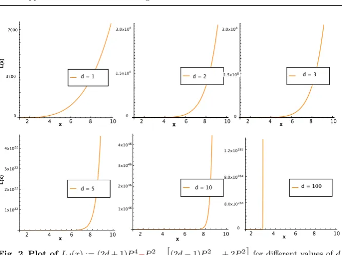
We numerically verify the inequality (39) in Figure 2; however, it is unclear to us how to prove it rigorously. We also recall that it is shown in Theorem
1 that fd(t) behaves like
√
d−1, which is an increasing function of d, as d
is sufficiently large. Motivated by these observations, we make the following prediction.
Conjecture 1 For any givent >0,fd(t) is an increasing function ofd.
We provide further numerical simulation to support this Conjecture by directly plottingfd(t) in Figure 1c.
Remark 2 We recall that in the casen= 2, the variabletis defined byt=1−yy, whereyis the fraction of strategy 1 and 1−yis that of strategy 2. Equivalently,
ycan be expressed in terms oftasy=1+tt. Hence one can also transform the statements of the theorem above (and later) in terms ofy. As has been shown in the beginning of Section2, the transformation fromy tot has the advantage that it transforms a complex equation (Eq. (8)) to a univariate polynomial equation (Eq. (10)). This enables us to exploit many available results and techniques from the literature of random polynomial theory. Moreover, from the relationship between f(t) and g(y), it follows that all the monotonicity properties with respect todare reserved for g2,d(see a numerical illustration
in Figure6).
4 General Cases
In this section, first we prove an estimate for the densityfn,2(t) similarly as
4.1 Two-player multi-strategy games
Theorem 6 (two-player multi-strategy games)
Assume that{Ai= (βi
j)j=1,···,n−1;i= 1, . . . , n−1} are independent random
vectors, then it holds that
fn,2(t) =π−
n
2Γ
n
2
if t1· · ·tn−1= 0 and (40)
fn,2(t)≤π−
n
2Γ
n
2
min
1, 1 nn2t1· · · tn−1
if t1· · ·tn−16= 0. (41)
As a consequence, for any tsuch thatt1· · ·tn−16= 0
lim
n→∞
fn,2(t)
π−n2Γ n
2
= 0. (42)
Proof According to [14, Theorem 3]
fn,2(t) =π−
n
2Γ
n
2
1
1 +
n−1
P
k=1
t2
k
n2
. (43)
The first assertion is then followed. Now suppose thatt1· · ·tn−1 6= 0. By the
Cauchy-Schwartz inequality, which statesPn
i=1an≥n(a1· · ·an)
1
n fornalln
positive numbersa1,· · ·, an, we have
1 +
n−1
X
k=1
t2k
!n2
≥nn2 t1 · · ·tn−1.
Therefore
fn,2(t)≤π−
n
2Γ
n
2
1
nn2 t1 · · · tn−1 .
On the other hand, since
1 +
n−1
P
k=1
t2k
n2
≥1, it follows that
fn,2(t)≤π−
n
2Γ
n
2
.
Therefore, we obtain (41).
Note that the expected number of internal equilibria for a two-player multi-strategy game is given by [14, Theorem 3]
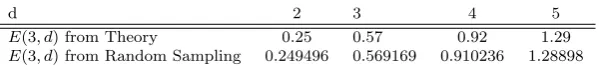
Table 1 Expected number of internal equilibria forn= 3 and differentd, as generated fromE(3, d) and from averaging over 106 random samples of the system of equation in2. In all cases, results from random samplings are slightly smallerE(3, d).
d 2 3 4 5
E(3, d) from Theory 0.25 0.57 0.92 1.29
E(3, d) from Random Sampling 0.249496 0.569169 0.910236 1.28898
Remark 3 In Theorem 6, we need an assumption that the random vectors
{Ai = (βi
j)j=1,···,n−1;i = 1, . . . , n−1} are independent. Recalling from
Sec-tion2that βi
k1,...,kn−1 =α
i
k1,...,kn−α
n
k1,...,kn, where α
i
i1,...,id−1 is the payoff of
the focal player, with i (1 ≤ i ≤ n) being the strategy of the focal player, and ik (with 1≤ik ≤nand 1 ≤k≤d−1) is the strategy of the player in
positionk. The assumption clearly holds forn= 2. Forn >2, the assumption holds only under quite restrictive conditions such asαn
k1,...,kn is deterministic
orαik1,...,kn are essentially identical. Note that the assumption is necessary to apply [15, Theorem 7.1]. Hence, to remove this assumption, one would need to generalize [15, Theorem 7.1]. This is difficult and is still an open problem [30,
31]. Nevertheless, since the system (3) has not been studied in the mathemati-cal literature, it is interesting on its own to investigate the number of real zeros of this system under the assumption of independence of {Ai}. As such, the
investigation not only provides new insights into the theory of zeros of systems of random polynomials but also gives important hint on the complexity of the game theoretical question, i.e. the number of expected number of equilibria. In Figure 7 and Table 1, we numerically compare the density function g3,d
and the expected number of equilibria E3,d computed from the theory with
the assumption and from samplings without the assumption. We observe that
g3,dhave the same shape (behaviour) in both cases. In addition, the values of
E3,dcomputed from samplings are slightly smaller than those computed from
the theory.
We now make a conjecture for the expected density and expected number of equilibria in a general multi-player multi-strategy game.
Conjecture 2 In a multi-player multi-strategy game, it holds that
fn,d∼(d−1)
n−1
2 and lim
d→∞
lnE(n, d) ln(d−1) =
n−1
2 . (44) We envisage that even a stronger statement holds
E(n, d)∼(d−1)n−21. (45)
a system ofn−1 random polynomials, each of the form
X
0≤k1,...,kn≤d−1, n
P
i=1
ki=d−1
βk1,...,kn s
d−1
k1, ..., kn
n
Y
i=1
xki
i , (46)
where the coefficientsβk1,...,kn are independent standard multivariate normal
distribution. Then according to [15, Section 7.2], the expected density and the expected number of real zeros are given by
fEP(t) =π−
n
2Γ
n
2
(d−1)
n−1 2
(1 +t·t)n2
, EEP = (d−1)
n−1
2 . (47)
These formula are direct consequences of Lemma1and the fact thatv(x)Cv(y) is a generating function, which generalises the univariate case
v(x)TCv(y) = X
0≤k1,...,kn≤d−1, n
P
i=1
ki=d−1
d−1
k1, ..., kn
n
Y
i=1
xkiyki = (1 +x·y)d−1.
As mentioned in Remark1, in our casev(x)TCv(y) is no longer a generating function due to the square of the multinomial coefficients. Motivated by this and Theorem 2 for the univariate case, we expect that the conjecture holds for the general case (i.e.d-player n-strategy normal evolutionary games).
4.2 Numerical results
In this section, we provide numerical simulations for all the (main) results obtained in the previous sections. The following figures are plotted. In the following list, (1) to (4) are to illustrate and confirm the analytical results obtained in the previous sections. The others, from (5) to (10), are numerical simulations for the games with large d and n. They also provide numerical support for Conjecture2.
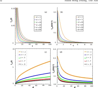
(1) fd(t) andfd(t)/(d−1) as functions oftfor different values ofd, see Figures
1a-b. Figure1a illustrates the fourth property in Proposition1 thatfd(t)
is increasing as a function oft. Figure1b explains the scaling by showing thatfd(t)/(d−1) is a bounded and decreasing function.
(2) fd(t) andfd(t)/(d−1) as functions ofdfor different values oft, see Figures
1c-d. These figures show that fd(t) increases withd while fd(t)/(d−1)
decreases, which are in agreement with Conjecture1and Theorem5. (3) fd(x) andfd(x)/(d−1) as functions of the frequencyx.
(5) f3,d(t1, t2) as a function oft= (t1, t2) for different values ofd, see Figures
5a-c.
(6) f3,d(t1, t2) as a function ofdfor different values oft= (t1, t2), see Figure
4a.
(7) f4,d(t1, t2, t3) as a function oft= (t1, t2, t3) for different values ofd, see
Figures5d-f.
(8) f4,d(t1, t2, t3) as a function ofd for different values of t= (t1, t2, t3), see
Figure4b.
(9) lnln(Ed(3−,d1)) as a function ofd, see Figure3b. (10) lnln(Ed(4−,d1)) as a function ofd, see Figure3c.
In Figures 5, we provide numerical results of fn,d(t) forn= 3 andn= 4.
We observe that the density function decreases withti (namely,t1 andt2 for
n= 3, andt1,t2andt3forn= 4) and increases withd. We conjecture that for
the generald-playern-strategy normal evolutionary game, the density function decreases withti and increases withd.
Figures 3b and3c support Conjecture2. From these two figures, one also can see the complexity of the problem when dincreases. We are able to run simulations for dup to 10000 forn= 2, up to 400 forn= 3 and only up to 20 forn= 4.
5 Discussion and outlook
How do equilibrium points in a general evolutionary game distribute if the pay-off matrix entries are randomly drawn, and furthermore, how do they behave when the numbers of players and strategies change? To address these impor-tant questions regarding generic properties of general evolutionary games, we have analyzed here the density function,fn,d, and the expected number of
(sta-ble) equilibrium points,E(n, d) (respectively,SE(n, d)), in a normald-player
n-strategy evolutionary game. We have shown, analytically and using numer-ical simulations, thatf2,d(t) monotonically decreases with twhile it increases
withd. The latter implies that, as the number of players in the game increases, it is more likely to see an equilibrium at a given pointt. We also proved that its scaling with respect to the number of players in a gamed, f2,d(t)
d , decreases
0 20 40 60 80 100 0.00 0.02 0.04 0.06 0.08 0.10 d=100 d=50 d=20 d=10 d=5 d=2
0 2 4 6 8 10 0.00 0.05 0.10 0.15 0.20 0.25 0.30 0.35
d=100 d=50 d=20 d=10 d=5 d=2
Ê ÊÊ ÊÊ ÊÊ ÊÊÊÊ ÊÊÊÊ ÊÊÊÊÊÊ ÊÊÊÊÊÊ ÊÊÊÊÊÊ ÊÊÊÊÊÊÊÊÊÊ
ÊÊÊÊÊÊÊÊ ÊÊÊÊÊÊÊÊ
ÊÊÊÊÊÊÊÊÊÊÊÊÊ ÊÊÊÊÊÊÊÊÊÊ ÊÊÊÊÊÊÊÊÊÊ ÊÊÊÊÊÊÊÊ ‡‡ ‡‡‡‡‡ ‡‡‡‡‡‡‡‡ ‡‡‡‡‡‡‡‡‡‡ ‡‡‡‡‡‡‡‡‡‡‡‡‡‡‡‡‡‡‡ ‡‡‡‡‡‡‡‡‡‡‡‡‡‡‡ ‡‡‡‡‡‡‡‡‡‡‡‡‡‡‡‡‡ ‡‡‡‡‡‡‡‡‡‡‡‡‡‡‡‡‡‡‡‡‡‡‡‡ ÏÏÏÏ ÏÏÏÏÏÏÏÏÏÏÏÏ ÏÏÏÏÏÏÏÏÏÏÏÏÏÏÏÏÏÏÏ ÏÏÏÏÏÏÏÏÏÏÏÏÏÏÏÏÏÏÏÏÏÏÏÏÏÏ ÏÏÏÏÏÏÏÏÏÏÏÏÏÏÏÏÏÏÏÏÏÏÏÏÏÏÏÏÏÏÏÏ ÏÏÏÏÏÏÏ ÚÚÚÚÚÚ ÚÚÚÚÚÚÚÚÚÚÚÚÚÚÚÚÚÚ
ÚÚÚÚÚÚÚÚÚÚÚÚÚÚÚÚÚÚÚÚÚÚÚÚÚÚÚÚÚÚÚÚÚÚÚÚÚÚÚÚÚÚÚÚÚÚÚ ÚÚÚÚÚÚÚÚÚÚÚÚÚÚÚÚÚÚÚÚÚÚÚÚÚÚÚÚÚ
ÙÙÙÙÙÙÙÙÙ
ÙÙÙÙÙÙÙÙÙÙÙÙÙÙÙÙÙÙÙÙÙÙÙÙÙÙÙÙÙÙÙÙÙÙÙÙÙÙÙÙÙÙÙÙÙ
ÙÙÙÙÙÙÙÙÙÙÙÙÙÙÙÙÙÙÙÙÙÙÙÙÙÙÙÙÙÙÙÙÙÙÙÙÙÙÙÙÙÙÙÙÙÙ
20 40 60 80 100
0 2 4 6 8 10
d-1
f
H
d
,t
L Ù t=0.9
Ú t=0.7 Ï t=0.5 ‡ t=0.3 Ê t=0.1 Ê Ê Ê Ê Ê Ê Ê Ê Ê Ê Ê ÊÊ Ê ÊÊ ÊÊÊÊÊ ÊÊÊÊÊÊÊÊÊ ÊÊÊÊÊÊÊÊÊÊÊÊÊÊÊÊÊ ÊÊÊÊÊÊÊÊÊÊÊÊÊÊÊÊÊÊÊÊÊÊÊÊÊÊÊÊÊÊÊÊÊÊÊÊÊÊÊÊ ÊÊÊÊÊÊÊÊÊÊÊÊ ‡ ‡ ‡ ‡ ‡ ‡ ‡ ‡ ‡‡ ‡‡‡‡‡‡‡ ‡‡‡‡‡‡‡‡‡‡‡‡‡‡‡‡‡‡‡‡ ‡‡‡‡‡‡‡‡‡‡‡‡‡‡‡‡‡‡‡‡‡‡‡‡‡‡‡‡‡‡‡‡‡‡‡‡‡‡‡‡‡‡‡‡‡‡‡‡‡‡‡‡‡‡‡‡‡‡‡‡‡‡ Ï Ï Ï Ï Ï ÏÏ ÏÏÏÏÏÏÏÏÏÏÏÏ ÏÏÏÏÏÏÏÏÏÏÏÏÏÏÏÏÏÏÏÏÏÏÏÏÏÏÏÏÏÏÏÏÏÏÏÏÏÏÏÏÏÏÏÏÏÏÏÏÏÏÏÏÏÏÏÏÏÏÏÏÏÏÏÏÏÏÏÏÏÏÏÏÏÏÏÏÏÏÏÏ Ú Ú Ú Ú ÚÚ ÚÚÚÚ ÚÚÚÚÚÚÚÚÚÚÚÚÚÚÚÚÚÚÚÚÚÚÚÚÚÚÚÚÚÚÚÚÚÚÚÚÚÚÚÚÚÚÚÚÚÚÚÚÚ ÚÚÚÚÚÚÚÚÚÚÚÚÚÚÚÚÚÚÚÚÚÚÚÚÚÚÚÚÚÚÚÚÚÚÚÚÚÚÚÚ Ù Ù Ù Ù ÙÙÙ ÙÙÙÙÙÙÙÙÙÙÙÙÙÙÙÙÙÙÙÙÙÙÙÙÙÙÙÙÙÙÙÙÙÙÙÙÙÙÙÙÙÙÙÙÙ ÙÙÙÙÙÙÙÙÙÙÙÙÙÙÙÙÙÙÙÙÙÙÙÙÙÙÙÙÙÙÙÙÙÙÙÙÙÙÙÙÙÙÙÙÙÙÙ
20 40 60 80 100
0.0 0.1 0.2 0.3 0.4 d f H d ,t LêH d -1 L
Ùt=0.9
Út=0.7 Ï t=0.5
‡ t=0.3 Êt=0.1
d d
t t
f2,d
(t)
f2,d
(t)/
(d
-1
)
f2,d
(t)/ (d -1 ) (a) (b) (c) (d)
d = 2 d = 5 d =10 d =20 d =50 d=100
d = 2 d = 5 d =10 d =20 d =50 d=100
t = .1 t = .3 t = .5
t = .7
t = .9
t = .1 t = .3 t = .5
t = .7
t = .9
0 20 40 60 80 100
0 20 40 60 80 100 0 20 40 60 80 100
0 2 4 6 8 10
0.2 0.1 0 0.3 0.10 0 0.05
f2,d
(t) 10 5 0 0.4 0.3 0.2 0.1 0.0
Fig. 1 (a) Plot of f2,d(t)and (b) off2,d(t)/(d−1) as functions oft, for different
values ofd. We observe that both functions decrease witht, which are in accordance with Proposition1. The second function is bounded from above, having maximum att= 0, which agrees with Theorem1.(c) Plot off2,d(t)and (d) off2,d(t)/(d−1)as functions ofd,
for different values oft. We observe thatf2,d(t) increases withd, whilef2,d(t)/(d−1)
decreases, which are in agreement with Conjecture1and Theorem5. All the results were obtained numerically using Mathematica.
works dealt with two-player games while we address here the general case (i.e. with arbitraryd).
Regarding the expected numbers of internal (stable) equilibrium points, first of all, as a result of the described monotonicity properties of the density function, we established analytically thatE(2, d) andSE(2, d) increase withd
while their scaled forms, E(2d,d) and SE(2d,d), decrease withd. Next, we proved a new upper bounds forn= 2, with arbitrary d:E(2, d).√d−1 ln(d−1). This upper bound is sharper than the one described in [14] (which is also the only known one, to the best of our knowledge). As a consequence, a sharper upper bound for the number of expected number of stable equilibria can be established:SE(2, d). 12√d−1 ln(d−1). More importantly, that allowed us to derive close-form limiting behaviors for such numbers: lim
d→∞
lnE(2,d) ln(d−1) =
1 2
and lim
d→∞
lnSE(2,d) ln(d−1) =
1
2. As such, apart from the mathematical elegance of
[image:23.595.74.389.70.353.2]2 4 6 8 10 1000 2000 3000 4000 5000 6000 7000 d=1
2 4 6 8 10
5.0¥107 1.0¥108 1.5¥108 2.0¥108 2.5¥108 3.0¥108 d=2
2 4 6 8 10
5.0¥107 1.0¥108 1.5¥108 2.0¥108 2.5¥108 3.0¥108
d=3
2 4 6 8 10
1¥1022 2¥1022 3¥1022 4¥1022
d=5
2 4 6 8 10
1¥1046 2¥1046 3¥1046 4¥1046
d=10
2 4 6 8 10
2.0¥10284 4.0¥10284 6.0¥10284 8.0¥10284 1.0¥10285 1.2¥10285 d=100
x x
x x x L (x )
2 4 6 8 10 2 4 6 8 10 2 4 6 8 10
2 4 6 8 10 2 4 6 8 10 2 4 6 8 10
d = 1 d = 2 d = 3
d = 5 d = 10 d = 100
[image:24.595.74.408.75.324.2]x 1x1022 2x10²² 3x10²² 4x10²² 1x1046 2x1046 3x1046 4x1046 1.2x10285 8.0x10284 8.0x10284 0 3.0x10⁸ 0 1.5x10⁸ 3.0x10⁸ 0 1.5x10⁸ 0 L (x ) 3500 7000
Fig. 2 Plot ofLd(x) := (2d+ 1)Pd4−Pd2−1 h
(2d−1)P2
d+1+ 2Pd2
i
for different values ofd. We observe thatLd(x) is always non-negative, thereby supporting Conjecture1, since the
inequalityLd(x)≥0 is the sufficient condition for the conjecture, as shown in Proposition 2 . Ê Ê ÊÊ Ê Ê Ê Ê Ê Ê Ê Ê Ê Ê Ê Ê Ê Ê Ê
ÊÊÊÊÊÊÊÊÊÊÊÊÊÊÊÊÊÊÊÊ Ê Ê Ê Ê Ê Ê Ê Ê Ê
Ê
0 2000 4000 6000 8000 10 000
0.0 0.1 0.2 0.3 0.4 0.5 d ln H E H 3, d LLê ln H d -1 L Ê Ê Ê Ê ÊÊ Ê ÊÊÊÊ Ê Ê ÊÊÊÊÊÊÊÊÊÊÊÊÊÊÊÊÊÊÊÊÊÊÊÊÊÊÊÊÊÊÊÊÊ Ê
Ê Ê Ê
Ê
50 100 150 200 250 300 350 400
0.0 0.2 0.4 0.6 0.8 1.0 d ln H E H 3, d LLê ln H d -1 L Ê Ê Ê ÊÊ
Ê ÊÊ Ê
Ê Ê ÊÊ Ê Ê Ê Ê
Ê
5 10 15 20
0.0 0.5 1.0 1.5 2.0 d ln H E H 4, d LLê ln H d -1 L ln (E(2 ,d ))/ ln (d -1 ) ln (E(3 ,d ))/ ln (d -1 ) ln (E(4 ,d ))/ ln (d -1 )
(a) (b) (c)
d d d
Fig. 3 Plot of lnln(Ed(−1)n,d) as functions of d, (a) for n= 2, (b) forn= 3and (c) for
n= 4. The results confirm the asymptotic behaviour forn= 2 as described in Theorem
2, and clearly support Conjecture 2 for the general case. All the results were obtained numerically using Mathematica.
studies of random evolutionary game theory [14,22,16]. Moreover, generalizing these formulas for the general case, i.e. when the number of strategiesnis also arbitrary, our conjecture that, lim
d→∞
lnE(n,d) ln(d−1) =
n−1
2 , is nicely corroborated by
[image:24.595.77.410.369.509.2]Ê Ê Ê Ê Ê Ê Ê Ê Ê Ê Ê Ê Ê Ê Ê Ê Ê Ê Ê Ê ‡ ‡ ‡ ‡ ‡ ‡ ‡ ‡ ‡ ‡ ‡ ‡ ‡ ‡ ‡ ‡ ‡ ‡ ‡ ‡
Ï Ï Ï Ï Ï Ï Ï Ï Ï
Ï Ï Ï
Ï Ï
Ï Ï
Ï Ï
Ï Ï
Ú Ú Ú Ú Ú Ú Ú Ú Ú Ú Ú Ú Ú Ú Ú Ú Ú Ú Ú Ú
Ù Ù Ù Ù Ù Ù Ù Ù Ù Ù Ù Ù Ù Ù Ù Ù Ù Ù Ù Ù
Á Á Á Á Á Á Á Á Á Á Á Á Á Á Á Á Á Á Á Á
· · · ·
5 10 15 20
0 100 200 300 400 500 600 d f H d ,t L ·0.5,0.5,0.5 Á0.3,0.5,0.5 Ù 0.1,0.5,0.5 Ú 0.1,0.3,0.5 Ï 0.1,0.1,0.5 ‡ 0.1,0.1,0.3 Ê 0.1,0.1,0.1 Ê Ê Ê Ê Ê Ê Ê Ê Ê Ê Ê Ê Ê Ê Ê Ê Ê Ê Ê Ê ‡ ‡ ‡ ‡ ‡ ‡ ‡ ‡ ‡ ‡ ‡ ‡ ‡ ‡ ‡ ‡ ‡ ‡ ‡ ‡
Ï Ï Ï Ï Ï Ï Ï
Ï Ï Ï
Ï Ï Ï Ï
Ï Ï Ï Ï
Ï Ï
Ú Ú Ú Ú Ú Ú Ú Ú Ú Ú Ú Ú Ú Ú Ú Ú Ú Ú Ú Ú
Ù Ù Ù Ù Ù Ù Ù Ù Ù Ù Ù Ù Ù Ù Ù Ù Ù Ù Ù Ù
5 10 15 20
0 20 40 60 80 100 d f H d ,t L Ù 0.5,0.5 Ú 0.3,0.5 Ï 0.1,0.5 ‡ 0.1,0.3 Ê 0.1,0.1 (t1,t2,t3) (t1,t2) f3,d (t) f4,d (t)
d d
(a) (b) 0.1,0.1 0.1,0.3 0.1,0.5 0.3,0.5 0.5,0.5 0.1,0.1,0.1 0.1,0.1,0.3 0.1,0.1,0.5 0.1,0.3,0.5 0.1,0.5,0.5 0.3,0.5,0.5 0.5,0.5,0.5
5 10 15 20 5 10 15 20
[image:25.595.74.407.71.248.2]0 20 40 60 80 100 0 600 500 400 300 200 100
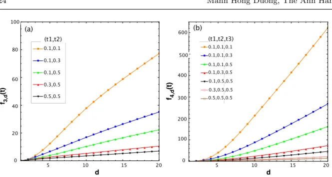
Fig. 4 Plot of (a) f3,d(t1, t2) for different values of (t1, t2)and (b) f4,d(t1, t2)for
different values of(t1, t2, t3), both as a function ofd. We observe that the functions increase withdwhile decrease withti, withi= 1,2 in panel (a) andi= 1,2,3 in panel (b).
All the results were obtained numerically using Mathematica.
the authors focused on the asymptotic behaviour of ESS with large support sizes, i.e. considering also equilibrium points which are not internal, in random pairwise games. In a similar context, in [25], the authors studied ESS but with support size of two, showing the asymptotic behaviors of such ESS when the number of strategies varies. Differently from all these works (which dealt exclusively with two-player interactions), our analysis copes with multi-player games. Hence, our results have led to further understanding with respect to the asymptotic behaviour of the expected number of stable equilibria for multi-player random games.
Last but not least, as the density functions we analyzed here are closely re-lated to Legendre polynomials, and actually, they are of the same form as the Bernstein polynomials, we have made a clear contribution to the longstanding theory of random polynomials [6,15,45,38](see again discussion in introduc-tion). We have derived asymptotic behaviors for the expected real zerosEBof a
random Bernstein polynomial, which, to our knowledge, had not been provided before. Note that the asymptotic behaviors and close forms of the expected real zeros of some other well-known polynomials have been derived by other authors. For instance, the Weyl polynomials forai:= i1!; the elliptic
polynomi-als or binomial polynomipolynomi-als withai:=
s
d−1
i
; and Kac polynomials with
ai := 1. The difference between the polynomial studied here (i.e. Bernstein)
with the elliptic case:ai=
d−1
i
are binomial coefficients, not their square root. In the elliptic case, v(x)TCv(y) = Pd−1
i=1
d−1
i
f3,d
(t)
f4,d
(t)
d=2 d=5 d=10
(a) (b) (c)
(d) (e) (f)
t1 t1
t1 t1 t1
t2 t2 t2
t2 t2 t2
0.5
1.0 0.0
0.5
1.0 0.0
0.5
1.0 0.0
0.5
1.0
0.5
1.0 0.0
0.5
1.0 0.0
0.5 1.0
0.0
0.5 1.0
0.0
0.5 1.0
0.0
0.5 1.0
0.0 0.5
1.0
0.0 0.5
1.0
0.0 1.0
0.0 0.5
8
0.0 4
20
0.0 10
1.0
0.0 0.5
10
0 5
40
0 20
[image:26.595.73.408.75.282.2]t1
Fig. 5 Plot of (a-c) f3,d(t1, t2)as a function of (t1, t2); and (d-f ) f4,d(t1, t2)as a
function of(t1, t2), for different values of t3. We observe that both functions increase withdwhile decrease withti, withi= 1,2 in panels (a)-(c) andi= 1,2,3 in panels (d)-(f).
In panels (a) and (d),d= 2; in panels (b) and (e),d= 5; in panels (c) and (f),d= 10. In panels (d)-(f), the surfaces, from bottom to top, correspond tot3 = 0.1, 0.3, 0.5, 0.7 and 10, respectively. All the results were obtained numerically using Mathematica.
the coefficients,v(x)TCv(y) =Pd−1
i=1
d−1
i
2
xiyi, is no longer a generating function. Indeed, as we notice, the Bernstein polynomials have been introduced for long, but due to such difficulties its direct analysis has been quite limited, see e.g. [3].
In short, our analysis has provided new understanding about the generic behaviors of equilibrium points in a general evolutionary game, namely, how they distribute and change in number when the number of players and that of the strategies in the game, are magnified.
6 Appendix
Detailed proofs of some lemmas and theorems in the previous sections are presented in this appendix.
6.1 Proof of Lemma3
0.2 0.4 0.6 0.8 1.0 0.4 0.6 0.8 1.0 1.2 1.4
0.2 0.4 0.6 0.8 1.0
0.3 0.4 0.5 0.6
d=5
d=4
d=3
d=2
g2, d (y ) g2, d (y )/ (d -1 ) y y
0.2 0.4 0.6 0.8 1.0 0.2 0.4 0.6 0.8 1.0
0.5 0.4 0.6 0.3 1.0 0.2
d = 2 1.4
0.2 0.4 0.6 0.8
1.2 d = 3
d = 4 d = 5
(a) (b)
Fig. 6 (a) Plot of g2,d(y) and (b) of g2,d(y)/(d−1) as functions ofy (note that t=1−yy), for different values ofd. We observe that both functions are symmetric about the liney= 1/2, in accordance with Lemma2. The first function increases withdwhile the second one decreases. All the results were obtained numerically using Mathematica.
d=2 d=3 d=5
0.5 1.0 0.0 0.5 1.0 0.0 0.5 1.0 0.0 0.5 1.0 0.0 0.5 1.0 0.0 0.5 1.0 0.0 0.5 1.0 0.0 0.5 1.0 0.0 0.5 1.0 0.0 0.5 1.0 0.0 0.5 1.0
0.0 0.5 1.0
0.0 0.0004 0.8 0.4 0.0002 3.0 1.5 0.0003 0.0002 0.0001 0.0003 0.0002 0.0001 1.2 0.6 y2 y2 y2 y1 y1 y1
y1 y1 y1
y2 y2 y2 g3 ,d (y1 ,y2 ) Pr o b a b il ity h is to g ra m
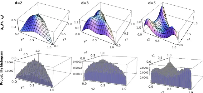
Fig. 7 (Top row)Plot of the density functiong3,d(y1, y2) for different values ofd(here
y1andy2are fractions of strategy 1 and 2, respectively, and 1−y1−y2is that of the third strategy).(Bottom row)Probability histograms plots of results from solving the system of equations2withn= 3 and for differentd, where the payoff entriesα’s are (independently) sampled from Gaussian distribution with mean 0 and standard deviation of 0.5 (106samples in total). The probability histograms have similar shapes tog3,d(y1, y2) (see also Table1). All the results were obtained numerically using Mathematica.
Proof (Proof of Lemma3)Letx=1+1−qq, from (28) we have
Pd
1 +q
1−q = 1 2d d X i=0 d i
21 +q
1−q −1
d−i1 +q
1−q+ 1
i = 1 2d d X i=0 d i
2 2q
1−q
d−i 2
1−q
i
= 1 (1−q)d
d X i=0 d i 2
qd−i
= 1 (1−q)d
d X i=0 d i 2
[image:27.595.71.410.72.250.2] [image:27.595.73.399.317.466.2]Therefore, d X i=0 d i 2
qi= (1−q)dPd
1 +q
1−q
.
By takingq=t2, we obtain (31).
6.2 Proof of Theorem3
Proof (Proof of Theorem3)
By taking the derivative of both sides in (31), we obtain
Md0+1(t) =−2t d(1−t2)d−1Pd
1 +t2
1−t2
+ 4t(1−t2)d−2Pd0
1 +t2
1−t2
=−2t dMd+1(t)
1−t2 + 4t(1−t 2)d−2P0
d
1 +t2
1−t2
.
It follows that
M0
d+1(t)
Md+1(t)
= −2t d 1−t2 +
4t
(1−t2)2
Pd0 Pd
1 +t2
1−t2
.
Now we compute the expression inside the square-root of the right-hand side of (32). We have
tM 0
d+1(t)
Md+1(t)
=−2t
2d
1−t2 +
4t2
(1−t2)2
Pd0 Pd
1 +t2
1−t2
, and tM 0
d+1(t)
Md+1(t)
0
=− 4t d
(1−t2)2+
8t(1 +t2)
(1−t2)3
Pd0 Pd
1 +t2
1−t2
+ 16t
3
(1−t2)4
Pd00Pd−(Pd0)
2
P2
d
1 +t2
1−t2
.
Substituting this expression into (33), we get
(2πfd+1(t))2=−
4d
(1−t2)2+
8(1 +t2)
(1−t2)3
Pd0 Pd
1 +t2
1−t2
+ 16t
2
(1−t2)4
Pd00Pd−(Pd0)2
P2
d
1 +t2
1−t2
.
(48) According to (27), the Legendre polynomialPdsatisfies the following equation
for allx∈R
−2xPd0(x) + (1−x2)Pd00(x) =−d(d+ 1)Pd(x).
As a consequence, we obtain
Pd00(x)
Pd(x)
= 1 1−x2
2xP 0
d(x)
Pd(x)
−d(d+ 1)
Substituting this expression into (48) withx= 1+1−tt22, we get
(2πfd+1(t))2=−
4d
(1−t2)2 +
8(1 +t2) (1−t2)3
Pd0 Pd
1 +t2
1−t2
+ 16t
2
(1−t2)4
1 1−1+t2
1−t2
2
21 +t
2
1−t2
Pd0 Pd
1 +t2
1−t2
−d(d+ 1)
−
P0
d
Pd
21 +t2
1−t2
= 4d
2
(1−t2)2 −
16t2
(1−t2)4
P0
d
Pd
21 +t2
1−t2
,
which is the claimed relation (33).
6.3 Proof of Theorem4
Proof (Proof of Theorem4)Using the following relation of the Legendre
poly-nomials for allx∈R
Pd0(x) =
d
x2−1(xPd(x)−Pd−1(x)),
we get
Pd0(x)
Pd(x)
= d
x2−1
x−Pd−1(x) Pd(x)
. (49)
In particular, takingx=1+1−tt22, we obtain Pd0
Pd
1 +t2
1−t2
= d
1+t2
1−t2
2
−1
1 +t2
1−t2 −
Pd−1
Pd
1 +t2
1−t2
=d(1−t
2)2
4t2
1 +t2
1−t2 −
Pd−1
Pd
1 +t2
1−t2
.
Substituting this expression into (33), we achieve
(2πfd+1(t))2=
4d2
(1−t2)2 −
d2
t2
1 +t2
1−t2 −
Pd−1
Pd
1 +t2
1−t2
2
,
which is (35).
6.4 Proof of Lemma4
Proof (Proof of Lemma 4) This lemma follows directly from [12] (Theorem
2.1) where the authors proved that
Pd(x)2−Pd+1(x)Pd−1(x) =
1−x2
d(d+ 1)
d X i=1 1 i +
d−1
X
i=1
1
i+ 1
i
X
j=1
(2j+ 1)Pj2(x)
,
6.5 Proof of Proposition2
Proof (Proof of Proposition2) We will prove that
fd2+2(t)−fd2+1(t)≥0 ⇐⇒ (38). (50)
From (35), we have
4π2(fd2+2(t)−fd2+1(t)) = 4(d+ 1)
2
(1−t2)2 −
(d+ 1)2
t2
1 +t2
1−t2 −
Pd
Pd+1
1 +t2
1−t2
2
− 4d
2
(1−t2)2 +
d2
t2
1 +t2
1−t2−
Pd−1
Pd
1 +t2
1−t2
2
= 4(2d+ 1) (1−t2)2 −
1
t2
1 +t2
1−t2 −
(d+ 1)Pd2−dPd−1Pd+1
PdPd+1
1 +t2
1−t2
×
(2d+ 1)1 +t
2
1−t2 −
(d+ 1)P2
d +dPd−1Pd+1
PdPd+1
1 +t2
1−t2
.
Thereforefd(t) is increasing as a function ofdif and only if
1 +t2
1−t2 −
(d+ 1)P2
d −dPd−1Pd+1
PdPd+1
1 +t2
1−t2
×
(2d+ 1)1 +t
2
1−t2 −
(d+ 1)P2
d +dPd−1Pd+1
PdPd+1
1 +t2
1−t2
≤ 4(2d+ 1)t
2
(1−t2)2 .
We re-write the expression above using the variablex, using the relationx2−
1 = 4t2
(1−t2)2, as follows
x−(d+ 1)P
2
d −dPd−1Pd+1
PdPd+1
(x)
×
(2d+ 1)x−(d+ 1)P
2
d +dPd−1Pd+1
PdPd+1
(x)
≤(2d+1)(x2−1).
(51) We now simplify this expression using the recursion relation of the Legendre polynomials, i.e.dPd−1= (2d+ 1)xPd−(d+ 1)Pd+1. Namely, we have
xPdPd+1−(d+ 1)Pd2+dPd−1Pd+1=xPdPd+1−(d+ 1)Pd2+ [(2d+ 1)xPd−(d+ 1)Pd+1]Pd+1
= (d+ 1)[−P2
d −P
2
d+1+ 2xPdPd+1]
and
(2d+ 1)xPdPd+1−(d+ 1)Pd2−dPd−1Pd+1
= (2d+ 1)xPdPd+1−(d+ 1)Pd2−[(2d+ 1)xPd−(d+ 1)Pd+1]Pd+1
= (d+ 1)(Pd2+1−Pd2).