Simultaneous fault models for the generation of efficient error detection mechanisms

(1)

warwick.ac.uk/lib-publications

Original citation:

Leeke, Matthew (2017) Simultaneous fault models for the generation of efficient error

detection mechanisms. In: 2017 IEEE 28th International Symposium on Software Reliability

Engineering (ISSRE'17), Toulouse, France, 23-26 Oct 2017. Published in: 2017 IEEE 28th

International Symposium on Software Reliability Engineering (ISSRE) ISBN 2332-6549.

Permanent WRAP URL:

http://wrap.warwick.ac.uk/93232

Copyright and reuse:

The Warwick Research Archive Portal (WRAP) makes this work by researchers of the

University of Warwick available open access under the following conditions. Copyright ©

and all moral rights to the version of the paper presented here belong to the individual

author(s) and/or other copyright owners. To the extent reasonable and practicable the

material made available in WRAP has been checked for eligibility before being made

available.

Copies of full items can be used for personal research or study, educational, or not-for profit

purposes without prior permission or charge. Provided that the authors, title and full

bibliographic details are credited, a hyperlink and/or URL is given for the original metadata

page and the content is not changed in any way.

Publisher’s statement:

© 2017 IEEE. Personal use of this material is permitted. Permission from IEEE must be

obtained for all other uses, in any current or future media, including reprinting

/republishing this material for advertising or promotional purposes, creating new collective

works, for resale or redistribution to servers or lists, or reuse of any copyrighted component

of this work in other works.

A note on versions:

The version presented here may differ from the published version or, version of record, if

you wish to cite this item you are advised to consult the publisher’s version. Please see the

‘permanent WRAP url’ above for details on accessing the published version and note that

access may require a subscription.

(2)

Simultaneous Fault Models for the Generation of

Efficient Error Detection Mechanisms

Matthew Leeke

Department of Computer Science, University of Warwick, Coventry, UK E-mail: [email protected]

Abstract—The application of machine learning to software fault injection data has been shown to be an effective approach for the generation of efficient error detection mechanisms (EDMs). However, such approaches to the design of EDMs have invariably adopted a fault model with a single-fault assumption, limiting the practical relevance of the detectors and their evaluation. Software containing more than a single fault is commonplace, with prominent safety standards recognising that critical failures are often the result of unlikely or unforeseen combinations of faults. This paper addresses this shortcoming, demonstrating that it is possible to generate similarly efficient EDMs under more realistic fault models. In particular, it is shown that (i) efficient EDMs can be designed using fault data collected under models accounting for the occurrence of simultaneous faults, (ii) exhaustive fault injection under a simultaneous bit flip model can yield improvements to EDM efficiency, and (iii) exhaustive fault injection under a simultaneous bit flip model can made non-exhaustive, reducing the resource costs of experimentation to practicable levels, without sacrificing resultant EDM efficiency.

Keywords-Detection; Error; Fault; Injection; Machine Learning

I. INTRODUCTION

The design of error detection mechanisms (EDMs) is integral to the development of dependable software systems [1]. EDMs are fundamentally concerned with the detection of erroneous software states. Once detected by an EDM, erroneous software states can be handled by error recovery mechanisms (ERMs) to maintain proper function. A failure to contain the propagation of erroneous state is known to make recovery more difficult, leading to a focus on the efficiency of EDMs through measures such as coverage and latency [2], [3].

The effectiveness of an EDM has been shown to depend on two factors. These factors are (i) the error detection predicate that it implements and (ii) its location in a software system [4]. This gives rise to two related problems. Firstly, the EDM design problem, which is concerned with the derivation of an error detection predicate over program variables that can be used for the detection of erroneous system states. Secondly, the EDM location problem, which is concerned with the identification of those software locations at which an EDM will be most effective. Though often treated as orthogonal for simplicity, the interaction of the implemented error detection predicate and the software location are demonstrably critical to the efficiency of an EDM [5], [6].

The efficiency of a particular EDM can be characterised by completeness and accuracy [4]. Completeness is the capability

of an EDM to detect erroneous states, i.e., its associated true positive rate. In contrast, accuracy is the capability of an EDM to avoid incorrectly detecting erroneous states, i.e., its associated false positive rate. An erroneous state is one that will lead to system failure if the error is not handled, where a failure is characterised as a violation of a system specification. An EDM that is complete and accurate is commonly known as a perfect detector. Due to implementation constraints, it is not generally possible to generate or guarantee the existence of a perfect detector for a particular software location [7].

The role of a fault model is to provide a means for analysing the response of software system to the presence a well defined set of faults, such that appropriate EDMs and ERMs can be designed to impart dependability. The assumption that faults do not occur simultaneously or interact is a limitation of many fault models and the software fault injection frameworks that implement them, not least because software containing more than a single fault are now commonplace [8]. In addition, numerous existing safety standards recognise that critical system failures are often the result of unlikely or unforeseen interactions combinations of faults [9].

It has been shown that efficient error detection predicates for EDMs can be designed through the application of machine learning algorithms to data sets generated during software fault injection [10]. This approach demonstrated, under a transient data value fault model, that it was possible to generate error detection predicates for specified locations with a true positive rate of nearly 100% and a false positive rate close to 0% for the detection of failure-inducing states. As is consistent with the overwhelming majority of software fault injection frameworks, these results were achieved under a single-fault assumption, calling into question their relevance in the context of real-world software systems.

(3)

including where non-exhaustive fault injection is performed in order to reduce the resource cost of conducting exhaustive experiments under a simultaneous fault model.

A. Contributions

This paper makes several specific contributions to the design of efficient EDMs for practical software. In particular, the research presented demonstrates that:

• Efficient EDMs can be designed using fault injection data

collected under models accounting for the occurrence of simultaneous faults;

• Exhaustive fault injection under a simultaneous bit flip

model can yield better EDM efficiency than under a non-simultaneous fault model;

• Exhaustive fault injection under a simultaneous bit flip

model can be made non-exhaustive without sacrificing the efficiency of the resultant EDMs, thus reducing the resource costs of experimentation to a practicable level. The overarching contribution of this paper is to demonstrate a practicable simultaneous fault model for the generation of efficient EDMs based on the application of machine learning to software fault injection data. In keeping with the simultaneous fault models employed, the generated EDMs are resilient to the single-fault assumption that limits the true efficiency and relevance of EDMs currently designed using such an approach.

B. Paper Structure

The remainder of this paper is structured as follows: Section II provides an overview of research relating to fault models for detector design. System III details the adopted system, data and fault models. Section IV provides an overview of how machine learning algorithms can be used to generate detection predicates for specified software locations. Section V provides details of the experiments conducted in this paper, including details of target software systems and applied machine learning algorithms. Section VI presents the results of the experiments conducted, alongside a discussion of their significance in the context of efficient error detector design. Section VII concludes the paper with a summary of findings and a brief discussion of future work in EDM design.

II. RELATEDWORK

A fault model has been shown to be composed of two parts, a local model and a global model [11]. The local fault model states the type of faults that are assumed to occur, whilst the global model dictates the extent to which the local fault model can occur. Ideally software should be examined under a representative workload and fault model. However, analyses under such circumstances can be impractical due to numbers of test cases or the fault space, particularly in the case of simultaneous fault models that demand consideration of fault combinations. Research has addressed these problems through leveraging parallel architectures in the execution of the large number of fault injection experiments [12], [13], though more scalable techniques have focused on sampling strategies for the test cases and error spaces [14], [15], [16].

The origin of the established bit flip fault model is in the diagnosis of hardware faults. In the context of software fault injection, bit flip and stuck-at fault models are often used to mimic transient and permanent hardware faults [17]. There has been much research on the representativeness of the faults captured by fault models used in software fault injection, motivated by results showing the issue can impact the validity of fault injection analysis. Results presented in [16] demonstrated that representativeness and resource efficiency in fault injection can be improved through the use of machine learning techniques and software metrics, a departure from fault-type focused approaches [18], [19].

The simultaneous fault models evaluated in this paper were proposed in [20] in response to a proliferation of software fault injection frameworks making the single-fault assumption, despite this being known to be unrealistic [8]. The models were developed on notions of coincidence and impact before being evaluated with regard to utility using metrics such as coverage and failure induction. Note that this focus is distinct from research exploring the simultaneous execution of fault injection experiments [21].

The focus of this paper is on the generation of efficient error detection predicates for EDMs under simultaneous fault models. The application of machine learning to EDM design is appealing because it does not assume the availability of a formal system specification [22] or rely on the experience of software engineers [23], the application of each has been shown to provide low efficiencies [24]. The approach is also applicable to practical software systems, as opposed to EDM design for smaller finite-state constructions [25]. Given that simultaneous fault models are more representative of practical software than models used to-date, the efficiencies presented in this paper provide a more representative commentary for the efficacy of machine learning as an EDM design approach.

III. MODELS

In this section the system, fault and data models used in this paper are described.

A. System Model

A software system S is taken to be a tuple, consisting of a

set of software modules,M1. . . Mn, and a set of connections.

A software module Mk consists of an import interface Ik,

an export interface Ek, a set of non-composite program

variables Vk and a sequence of actions Ak1. . . Aki. Each

program variable inVkhas a domain of values. Each action in

Ak1. . . Akimay read or write to a subset ofVk. Two software

modules Mk and Ml are connected if the export interface

of Mk is matched with the import interface of Ml, i.e., a

connection exists ifEk is matched with Il. Thus, a software

systemS = (M OD, CON), where M OD ={M1. . . Mn},

andCON ={(Ma

k, Mla)}, where Mk exports to the import

interface ofMlover connectiona. The adopted system model

(4)

B. Fault Models

The simultaneous fault models described were developed to improve software fault injection by overcoming the single-fault assumption, thus permitting more meaningful analyses [20]. As the fault injection conducted in [20] focused on the point of entry to modules, the fault injection experiments in this paper focus on generating EDMs at the entry points to modules, an approach supported by existing research [26]. To maintain compatibility with existing research, software state was characterised by all variables in scope at the point of fault injection. All variables in scope were subject to fault injection experiments. The described fault models were systematically applied to exhaustive combinations of variables in scope, e.g.,

ifnvariables were in scope then each fault model was applied

to every k-combination for 1≤k≤n.

Fault models were used only for the collection of software fault injection data that served as input to the machine learning algorithms, i.e., the machine learning used took no account of the fault model or data generation process.

Bit Flip (BF)

The BF fault model injects a single bit flip fault into the representation of a single variable in each fault injection experiment, thus incorporating the single-fault assumption and providing a broad basis for comparison with simultaneous fault models. This is a well established model for software fault injection, being consistent with fault model used in previous work on the application of machine learning for the generation of efficient EDMs [10], [17], [27].

Simultaneous Fuzzing (FuzzFuzz)

A single fuzzing injection involves the modification of a variable value to a random value of the same bit length. If fuzzing were simultaneously applied to a single variable, the result would not differ from a single fuzzing injection. This means there is no need to consider injection in the same variable. Rather, under the FuzzFuzz model, the values of more than one target variable are subject to fuzzing. Exhaustive software fault injection using fuzzing is impractical, since the number of possible injection values

for an n-bit variable v is 2n_{. For this reason we restrict}

experimentation to a fixed number of fault injections for each variable combination simultaneous targeted under FuzzFuzz, adhering to the experimental guidance derived from results presented in [20] and [28].

Simultaneous Bit Flip (SimBF)

The SimBF fault model performs fault injections at the resolution of a single variable. In the original formulation of the model, only combinations of two bit flips were con-sidered [20]. To ensure that initial experiments under this model could be said to exhaustive, bit flip fault injection was

systemically applied to exhaustive k-combination

combina-tions of bits in each variable representation. Coupled with

the exhaustive consideration of k-combinations of variables

in which to inject, this fault model requires a large number

of experiments to consider exhaustively. It should be noted that this large number of experiments is not practical at larger scales. An exhaustive approach is initially adopted in this paper to set a standard for EDM efficiencies, such that the efficiencies of EDMs generated by non-exhaustive approaches can be better understood.

C. Data Model

In the application of machine learning, data pertaining to a real-world process is typically modelled as a set of entities, their attributes and their known relationship to other entities. This is commonly known as the relational model of data. Data generated, hence stored, within such a relational data model is a sample of all the data that may be generated by the process. Often, rather than being interested in the retrieval of stored data, it is more interesting and useful to be able to forecast behaviours of the process not previously encountered or derive knowledge about the process if the process itself is not well understood. For example, in the context of the research presented in this paper, it is interesting to understand how a software under test, as the process modelled, is likely to behave when confronted with an injected fault.

IV. EDM GENERATIONUSINGMACHINELEARNING

Recall that the effectiveness of an EDM has been shown to depend the error detection predicate it implements and its location in software. If the software location is known, EDM generation entails the generation of an error detection predicate for implementation, typically as a runtime assertion.

The premise of using machine learning on fault injection data is that the data generated during fault injection analysis captures aspects of the relationships between current software states and future system failure. Based on the software states sampled during fault injection analysis, machine learning algorithms can be applied to learn the relationship between the execution state of the software, as embodied by the values of all variables in scope, and the notion of system failure.

As data collected during fault injection analysis provides an indication of whether a sampled software state resulted in a failure, the generation of a an error detection predicate from that data is a supervised learning problem. Data is assumed to

exist as a single relation consisting of a set ofninput attributes

that define ann-dimensional space called the Instance Space,

I. Every point in I is a potential state of the process being

modelled. In supervised learning a data mining algorithm is

tasked with learning a good approximation,fˆ, of an unknown

functionf, referred to as the target function, given a training

data set, T ⊆I, consisting of the N pairs hxi, f(xi)i. If the

(5)

the concept, are referred to as positive instances. Instances not belonging to the concept are referred to as negative instances. A process for EDM generation using machine learning on fault injection data is described in [10]. The process consists of four generic stages, followed by the evaluation of detection efficiency. The stages of the process, as reflected in Sections IV-A- IV-E, are: Data Collection ( IV-A), Data Preprocessing ( IV-B), Model Generation ( IV-C), Model Refinement ( IV-D), and Model Evaluation ( IV-E).

A. Data Collection

The fault injection process in this context is a means for the generation of data that captures the functional relationship between software state and system failure. To a large extent, the fault model applied in fault injection dictates the nature and extent of the exploration of software states, making the selection and robust application of a representative fault model imperative. The exploration of simultaneous fault models is the fundamental concern of this paper, focusing fault injection analysis on the fault models described in Section III.

B. Data Preprocessing

Data preprocessing is performed to transform collected fault injection data, the format of which varies by fault injection framework, into a suitable relational data format for learning. This transformation provides an opportunity to address issues such as class imbalance, which can prevent the development of reliable predictive models in concept learning problems [29]. In particular, data sets resulting from fault injection analysis often contain significantly fewer instances of system failure than instances of successful software execution. This feature of the fault injection data must be accounted for before predictive models are generated. This is an appropriate point at which to tackle this problem because most approaches to address class imbalance require the generation of derivative data sets, a task made simpler if these are produced during data transformation.

C. Model Generation

Symbolic pattern learning algorithms are an effective class of algorithm for the generation of error detection predicates, not least because their output can easily be interpreted as first-order predicates. This paper applies the decision tree induction and rule induction as machine learning algorithms, since these have been shown to be capable of generating efficient, in some cases near-perfect, predicates for EDMs. The function approximation learnt, referred to as the model, by a classification algorithm needs to be evaluated, in order to obtain a measure of the expected accuracy of the model on unseen data. Typically the accuracy of a model is measured by the percentage of test data instances correctly classified, hence most algorithms seek to learn hypotheses that minimise the number of errors. Conveniently this is consistent with the notions of accuracy and completeness used in the measurement of EDM efficiency. However, this implicitly assumes that all types of misclassification incur an equal cost, which is not always the case. For example, in the case of safety-critical

TABLE I: The general confusion matrix for concept learning.

Predicted Class

Pos. Neg. Margina Sum

Actual

Pos. TP FN npos

Neg. FP TN nneg

Marginal Sums nˆpos nˆneg n

software, a model incorrectly classifying a failure-inducing state will typically result in a much more significant cost than a non-failure-inducing state being classified as failure-inducing.

D. Model Refinement

The models generated are refined by varying the parameters associated with the configuration of the associated machine learning algorithms. In practice this is realised by repeating the execution of the algorithms under different configurations on the undersampled and oversampled data sets generated during preprocessing in order to establish an algorithm configuration and data set which yields the most efficient error detection predicate. Achieving a perfect detector may not be possible for a given location. This is not a direct limitation of the machine learning approach, rather it is a theoretical constraint of the EDM design problem [7].

E. Model Evaluation

The predictions of a model for a data set under test can be cross-tabulated with the actual classes assigned to the instances by the target function to produce a confusion matrix. Table I shows the general form of a confusion matrix for concept learning. TP is the number of positives instances labelled

as positive instances by fˆ, known as true positives, whilst

FN is the number of positive instances labelled as negative, known as false negatives. FP is the number of negative instances labelled as positive, known as false positives, whilst TN is the number of negative instances labelled as negative,

known as true negatives. Finally,npos/nnegare the number of

positive/negative instances in the test data and nˆpos/ˆnneg are

the number of instances predicted as positive / negative. Aggregate measures of model quality seek to balance the concerns of the confusion matrix shown in Table I. The most basic of these measures are true negative rate (TNR) and true positive rate (TPR).

T N R= T N

T N+F P (1)

T P R= T P

T P+F N (2)

These measures give rise to ROC analysis, which is based on a plot in two dimensions where each model is a point defined by the coordinates (1-TNR, TPR). Note that (1-TNR) is also referred to as the false positive rate (FPR).

F P R= F P

T N+F P (3)

(6)

obtained by joining these points to (0,0) and (1,1) is arguably the most common measure of model performance. As the focus of this paper is on evaluating the impact of more realistic fault models on EDM efficiency, understood as their accuracy and completeness, AUC is used in model evaluation.

AU C= T P R−F P R+ 1

2 (4)

Since misclassification costs are likely to vary in the context of dependable software systems, steps must be taken to ensure that high AUC values are not achieved through the neglect of accuracy or completeness. With this in mind, TPR and FPR are also considered in model evaluation.

V. EXPERIMENTALSETUP

In this section the experimental approach employed in this paper is explained, including coverage of the target software systems and machine learning algorithms.

A. Data Collection

Four target software systems were subject to experimentation. Five randomly chosen modules in each system were chosen for experimentation. Failures were identified through comparison with a fault-free execution, where any discrepancy in output or the completion of the test case was deemed a failure.

7-Zip Archiving Utility (7Z):7-Zip is a compression utility that supports archiving and encryption [30]. 7-Zip is widely-used, modular, written in C/C++ and has been designed, developed and maintained by a community of software engineers. Most source code and resources for 7-Zip are freely available under the GNU Lesser General Public License. A single file archiving procedure was executed as a test case.

FlightGear Flight Simulator (FG): FlightGear is an open source flight simulator [31]. The software is modular, contains more than 250,000 lines of C/C++ and simulates a safety critical situation. All source code and resources for FlightGear Flight Simulator are available under the GNU General Public License. A takeoff procedure was executed as a test case.

MP3Gain (MG): MP3Gain is an open source volume normaliser [32]. MP3Gain is modular, written in C/C++ and has been predominantly developed by a single software engineer. All source code for MP3Gain is available under the GNU General Public License. A single file volume normalisation procedure was executed as a test case.

ImageMagick (IM): ImageMagick is an open source image editing suite that can be utilised from the command line [33]. ImageMagick is modular, written in C/C++ and has been de-signed, developed and maintained by a small team of software engineers. All source code and resources for ImageMagick are available under the Apache 2.0 license. A colour balancing, crop and scaling image procedure was executed as a test case.

TRUE (148) TRUE (249)

FALSE (126)

FALSE (59)

TRUE (119)

TRUE (49) TRUE (52)

VarOne

VarThree VarTwo

VarSix VarFour

VarFive

VarSix

VarFive

VarSix

VarSeven

VarTwo

VarFour

< 43.32 ≥ 43.32

< 42 ≥ 42

> 523 ≤ 523 > -0.99 ≤ -0.99

> 0 ≤ 0 > 1 ≤ 1 > 522 ≤ 522

[image:6.612.318.558.55.235.2]

> 0 ≤ 0 > 10 ≤ 10

Fig. 1: Example decision tree generated under C4.5 [10].

B. Data Preprocessing

The data generated during fault injection was stored using the PROPANE logging format, though the lack of simultaneous fault model support meant a bespoke framework was used for the injection of faults [34]. This meant a format transformation between the PROPANE logging format and the Attribute Relation File Format (ARFF) used by the Weka Data Mining suite for model generation [35]. In this format, each variable in scope is an attribute and the class label identifies failures.

There are two approaches for addressing class imbalanced data sets. Either the data distribution can be implicitly changed or the data set can be resampled to make the class distribution more uniform. The former is commonly achieved through the association of weights with training examples [36], [37]. The main problem with this in the context of EDM generation is the identification of appropriate weights. Resampling to make the class distribution more uniform does not suffer from this issue, since it is achieved by oversampling the minority class or, more commonly, undersampling the majority class [38], [39]. Hence, Synthetic Minority Oversampling Technique (SMOTE) was used to address class imbalance. This approach generates synthetic samples for minority classes along the line segment joining an example to k-minority class nearest neighbours, with cross validation being used to set the level of oversampling and undersampling of the majority and minority classes [40], [41].

C. Model Generation

The Weka Data Mining suite provided the implementation of the algorithms used in model generation [35]. In particular, Weka provided implementation of the C4.5 decision tree induction and Repeated Incremental Pruning to Produce Error Reduction (RIPPER) algorithms [42], [43].

(7)

edge emanating from a decision node is labelled with one of the unique values in the domain of the attribute labelling the decision node. A leaf node is labelled using one of the classification labels. Each path of the tree from the root node to a leaf node is interpreted as a set of conjunctive expressions that lead to the classification label at the leaf node. The algorithm performs a greedy search of the space of all possible trees choosing decision node attributes that maximise the reduction in entropy of the class label.

Rule Induction operates in distinct phases. Specifically, beginning with with the least represented class label, the algorithm repeatedly grows and prunes rules until there are no positive examples left or the error rate is greater than 0.5. A rule is grown by incorporating greedy conditions until the rule is perfectly accurate. This is done by attempting to incorporate every possible value of each attribute and selecting the condition providing most information gain. A rule is pruned by removing any final sequences of antecedents according to a fixed pruning metric, providing some facility to incorporate domain knowledge and combat overfitting.

D. Model Refinement

A total of 20 undersampling and 15 oversampling levels were used in model refinement. These levels were distributed over [5,100] and [100,1500] for undersampling and oversampling respectively. The number of nearest neighbours considered in the sampling process were uniformly distributed over [1,15]. These ranges were chosen arbitrarily to provide insight into achievable improvement, as opposed to performing a search of configurations in pursuit of optimal model performance.

E. EDM Evaluation

Following the application of each machine learning algorithm to each fault injection data set, 10-fold cross validation was used to generate the confusion matrices. The use of 10-fold cross validation meant that the entries in each data set are partitioned into 10 stratified samples, then for each cross validation run, one of these partitions is used as a test sample, whilst the other nine partitions are used as the training set for a particular machine learning algorithm.

VI. RESULTS

Following the application of the machine learning algorithms to each of the generated fault injection data sets, including undersampled and oversampled data, 10-fold cross validation was used to generate the confusion matrix for each algorithm on each data set. The use of 10-fold cross validation meant that the entries in each data set are partitioned into 10 stratified samples, then for each cross validation run, one of these partitions is used as a test sample, whilst the other nine are used as the training set for a particular algorithm.

Sections VI-A- VI-E present results for the error detection predicates learnt under varying fault models. For each of the machine learning algorithms applied, results are presented for the error detection predicates generated before and after optimisation. All optimisation performed in this paper was

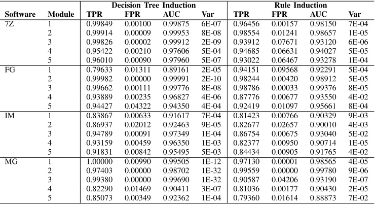
achieved through varying parameters that are independent of any data mining algorithm, i.e., the data set sampling levels applied prior to model generation. This ensures that the same refinement process can be applied regardless of the selected algorithm. In the tables presented in Sections VI-A to VI-E, the FPR and TPR columns give the mean false positive and true positive rates taken across ten cross validations. A true positive corresponds to a model correctly identifying a failure-inducing state, whereas a false positive corresponds to a model incorrectly detecting a state as being failure-inducing. The AUC column shows the area under the ROC curve, the aggregate measure of efficiency that balances the consideration of TRP against FPR. The Var column gives the AUC variance across all ten cross validations, providing an indication of how consistently efficient models were generated.

A. BF Fault Model

Evaluating error detection predicates generated under the non-simultaneous BF fault model provides a convenient benchmark for the analysis of simultaneous fault models. It is desirable for error detection predicates generated under any simultaneous fault models to maintain the high efficiency and low variance that is associated with error detection predicates generated by the same approach under a non-simultaneous fault model.

Table II demonstrates levels of efficiency commensurate with those previously observed when using decision tree induction and rule induction algorithms to generate error detection predicates [10]. The hallmarks of these algorithms for predicate generation can be seen in the consistently high AUC values, ranging from 0.89161 to 0.99991 for decision tree induction and from 0.88873 to 0.99780 for rule induction. Decision tree induction is the better performing of the two model generation algorithms, with higher TPR in most cases, another observation that is commensurate with existing work in machine learning for error detection predicate generation. An AUC of 0.90411 or higher can be found for every module subject to analysis, an indication that the predicates generated are effective classifiers for failure inducing states. It can also be observed that whilst some generated detectors were perfect

with respect to accuracy (T P R = 1) and some perfect with

respect to completeness (F P R = 0), no perfect detector

(T RP = 1,F P R= 0) was generated.

B. FuzzFuzz Fault Model

The FuzzFuzz model is the first simultaneous fault model to be analysed. As the space of possible fault injections under the FuzzFuzz fault model makes exhaustive injections impractical,

since the number of possible injection values for an singlen

-bit variablev is2n_{, experimentation was restricted to a fixed}

number of fault injections for each combination of variables simultaneously targeted. Table III and Table IV present results where the number of fault injections for each combination of variables simultaneously targeted is 30 and 100 respectively.

(8)

[image:8.612.122.493.71.273.2]

TABLE II: The efficiency of error detection predicates generated and evaluated under the BF fault model.

Decision Tree Induction Rule Induction

Software Module TPR FPR AUC Var TPR FPR AUC Var

7Z 1 0.99849 0.00100 0.99875 6E-07 0.96456 0.00157 0.98150 7E-04

2 0.99914 0.00009 0.99953 8E-08 0.98554 0.01241 0.98657 1E-05

3 0.99826 0.00002 0.99912 2E-09 0.93912 0.07671 0.93120 6E-06

4 0.95422 0.00210 0.97606 5E-04 0.94685 0.06631 0.94027 5E-05

5 0.96010 0.00090 0.97960 5E-07 0.93022 0.06467 0.93278 1E-04

FG 1 0.79633 0.01311 0.89161 2E-05 0.94151 0.09568 0.92291 5E-04

2 0.99982 0.00000 0.99991 2E-10 0.98244 0.00420 0.98912 5E-05

3 0.99662 0.00111 0.99776 8E-08 0.98786 0.00033 0.99376 8E-05

4 0.93889 0.00235 0.96827 4E-06 0.87776 0.00677 0.93550 4E-02

5 0.94427 0.04322 0.94350 4E-04 0.92419 0.01097 0.95661 8E-04

IM 1 0.83867 0.00633 0.91617 7E-04 0.81423 0.00766 0.90329 9E-03

2 0.86937 0.02012 0.92463 9E-05 0.82677 0.02657 0.90010 4E-03

3 0.94789 0.00091 0.97349 1E-04 0.86754 0.00675 0.93040 5E-02

4 0.93159 0.00459 0.96350 1E-03 0.82377 0.00950 0.90714 1E-05

5 0.91831 0.00842 0.95495 5E-03 0.84434 0.00905 0.91765 4E-02

MG 1 1.00000 0.00990 0.99505 1E-12 0.97130 0.00001 0.98565 4E-05

2 0.97403 0.00000 0.98702 1E-32 0.99559 0.00000 0.99780 9E-06

3 0.99380 0.00000 0.99690 1E-32 0.90587 0.04206 0.93190 7E-07

4 0.82290 0.01469 0.90411 3E-07 0.81036 0.00177 0.90430 2E-05

[image:8.612.127.489.314.516.2]

5 0.85073 0.00349 0.92362 1E-04 0.79360 0.01614 0.88873 7E-02

TABLE III: The efficiency of error detection predicates generated and evaluated under the FuzzFuzz fault model with 30 fault injection experiments for each combination of target variables.

System Module TPR FPR AUC Var TPR FPR AUC Var

7Z 1 0.64430 0.17731 0.73350 5E-02 0.55872 0.28880 0.63496 7E-03

2 0.59887 0.23541 0.68173 7E-02 0.51426 0.28823 0.61302 2E-03

3 0.54452 0.04431 0.75011 9E-04 0.52676 0.04493 0.74092 7E-03

4 0.63089 0.08624 0.77233 9E-02 0.50364 0.08907 0.70729 9E-03

5 0.56538 0.00793 0.77873 1E-02 0.50114 0.00960 0.74577 9E-03

FG 1 0.67200 0.04847 0.81177 3E-02 0.53404 0.03964 0.74720 6E-03

2 0.61528 0.00626 0.80451 5E-03 0.53584 0.01239 0.76173 6E-03

3 0.52155 0.06680 0.72738 1E-02 0.51829 0.06821 0.72504 9E-04

4 0.69746 0.08621 0.80563 6E-02 0.58829 0.08780 0.75025 7E-03

5 0.53417 0.00917 0.76250 1E-03 0.51322 0.04446 0.73438 4E-03

IM 1 0.61181 0.00258 0.80462 5E-02 0.51907 0.04399 0.73754 6E-02

2 0.61151 0.04591 0.78280 8E-03 0.60607 0.04972 0.77818 4E-03

3 0.64896 0.01207 0.81845 2E-02 0.54398 0.06983 0.73708 5E-03

4 0.66317 0.02439 0.81939 3E-03 0.53377 0.04608 0.74385 5E-03

5 0.62518 0.00411 0.81054 8E-04 0.50813 0.00966 0.74924 1E-03

MG 1 0.53590 0.00987 0.76302 1E-03 0.50873 0.03244 0.73815 9E-03

2 0.63777 0.00879 0.81449 5E-04 0.54761 0.00956 0.76903 8E-02

3 0.55767 0.01651 0.77058 1E-03 0.51580 0.12764 0.69408 4E-03

4 0.57714 0.03535 0.77090 8E-03 0.52553 0.08434 0.72060 4E-02

5 0.52629 0.00890 0.75870 1E-02 0.50150 0.01485 0.74333 5E-02

Table IV demonstrates that it is possible to generate efficient error detection predicates under a fuzzing model. Note that the efficiencies of these error detection predicates are below those observed under the BF fault model, both in this paper and in existing research, with an aggregate mean AUC of 0.90493.

It should be remembered that the levels of performance are not to the detriment of the simultaneous fault model, since the associated the set of injected faults will result in greater perturbation of software state. Intuitively, the impact of fuzzing for a fixed number of repeats is to incur a less structured and thorough exploration of erroneous software state, thus making it more difficult for a machine learning algorithm to discern the relationship between erroneous software state and system failure. This intuition is substantiated by the marked improvement the efficiencies of the error detection predicates

generated using a larger number of fault injection experiments for each combination of target variables.

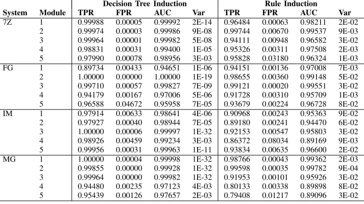
C. SimBF Fault Model

The SimBF fault model is the most computationally expensive set of experiments presented in this paper, since bit flip fault injection was applied to exhaustive combinations of bits in each variable representation across exhaustive combinations of variables. Whilst polynomial in bit representation and the number of variables, conducting this number of experiments in the development of most software systems is impractical. Despite this, the efficiencies shown are the strongest presented and warrant consideration regardless of the cost incurred.

(9)

[image:9.612.126.489.83.284.2]

TABLE IV: The efficiency of error detection predicates generated and evaluated under the FuzzFuzz fault model with 100 fault injection experiments for each combination of target variables.

7Z 1 0.92298 0.08920 0.91689 7E-05 0.85316 0.00538 0.92389 9E-02

2 0.89798 0.00161 0.94819 3E-04 0.81497 0.00887 0.90305 2E-02

3 0.84798 0.00944 0.91927 2E-05 0.79370 0.01118 0.89126 6E-01

4 0.89089 0.06959 0.91065 4E-03 0.79718 0.00204 0.89757 9E-03

5 0.83002 0.00933 0.91035 3E-03 0.78101 0.00145 0.88978 7E-02

FG 1 0.75158 0.02956 0.86101 5E-06 0.77264 0.01997 0.87634 9E-02

2 0.88952 0.00260 0.94346 1E-06 0.75132 0.00987 0.87073 1E-02

3 0.91492 0.06680 0.92406 9E-07 0.83180 0.06126 0.88527 2E-03

4 0.89191 0.00876 0.94158 5E-05 0.88171 0.03874 0.92149 1E-02

5 0.83837 0.00714 0.91562 7E-05 0.80233 0.02890 0.88672 1E-02

IM 1 0.78233 0.00126 0.89054 7E-02 0.81423 0.04303 0.88560 2E-01

2 0.71151 0.00638 0.85257 2E-03 0.82677 0.02987 0.89845 9E-02

3 0.83389 0.00342 0.91524 2E-03 0.86754 0.06319 0.90218 6E-02

4 0.73310 0.02439 0.85436 8E-04 0.82377 0.04415 0.88981 2E-02

5 0.81016 0.00330 0.90343 2E-02 0.84434 0.00750 0.91842 9E-04

MG 1 0.82051 0.00583 0.90734 1E-05 0.97130 0.00761 0.98185 7E-02

2 0.84187 0.00035 0.92076 1E-03 0.99559 0.00319 0.99620 5E-03

3 0.77253 0.00716 0.88269 4E-03 0.90587 0.09489 0.90549 2E-02

4 0.76022 0.01853 0.87085 1E-03 0.81036 0.03768 0.88634 1E-02

5 0.82237 0.00299 0.90969 2E-03 0.79360 0.01193 0.89084 4E-02

TABLE V: The efficiency of error detection predicates generated and evaluated under the SimBF fault model.

7Z 1 0.99988 0.00005 0.99992 2E-14 0.96484 0.00063 0.98211 2E-02

2 0.99974 0.00003 0.99986 9E-08 0.99744 0.00670 0.99537 9E-03

3 0.99964 0.00001 0.99982 5E-08 0.94111 0.00948 0.96582 3E-02

4 0.98831 0.00031 0.99400 1E-05 0.95326 0.00311 0.97508 2E-03

5 0.97990 0.00078 0.98956 3E-03 0.95828 0.03180 0.96324 1E-03

FG 1 0.89734 0.00433 0.94651 1E-06 0.94151 0.00136 0.97008 7E-03

2 1.00000 0.00000 1.00000 1E-19 0.98655 0.00360 0.99148 5E-02

3 0.99710 0.00057 0.99827 7E-09 0.99121 0.00020 0.99551 3E-02

4 0.94179 0.00167 0.97006 5E-06 0.91728 0.00310 0.95709 1E-03

5 0.96588 0.04672 0.95958 7E-05 0.93679 0.00224 0.96728 8E-02

IM 1 0.97914 0.00633 0.98641 4E-06 0.90968 0.00243 0.95363 9E-02

2 0.97927 0.00040 0.98944 7E-05 0.89180 0.00241 0.94470 6E-02

3 1.00000 0.00006 0.99997 1E-32 0.92153 0.00547 0.95803 3E-02

4 0.98926 0.00459 0.99234 3E-03 0.86372 0.08034 0.89169 9E-03

5 0.99956 0.00031 0.99963 1E-11 0.93834 0.00635 0.96600 2E-02

MG 1 1.00000 0.00004 0.99998 1E-32 0.98766 0.00043 0.99362 2E-03

2 0.99855 0.00000 0.99928 1E-32 0.99598 0.00035 0.99782 9E-04

3 0.99964 0.00000 0.99982 1E-32 0.91953 0.00101 0.95926 3E-02

4 0.94480 0.00235 0.97123 4E-03 0.80133 0.00338 0.89898 8E-02

5 0.95439 0.00126 0.97657 2E-03 0.79408 0.01217 0.89096 3E-02

predicated associated with several other modules, most notably IM-3 and MG-1, are near perfect. The aggregate mean AUC for decision tree induction is 0.98861, meaning that it is once again the better performing of the two model generation algorithms. This is higher than the 0.93667 recorded under the BF fault model, despite SimBF being the stronger of the two fault models in terms of the faults imposed / perturbation of software state. Supporting preliminary findings in [10], this is an indication that a comprehensive exploration of erroneous software states is fundamental to the generation of efficient error detection predicates using machine learning.

D. Simultaneous Fault Model Efficacy

Although simultaneous fault models are proposed to be more representative and cross validation allow the efficiency of the generated error detection predicates to be evaluated, gaining

insight into the efficacy of simultaneous fault models is challenging. It is natural to consider the extent to which the error detection predicates generated under a simultaneous fault model can account for the set of faults injected under a non-simultaneous model, since the latter is commonly used to inform EDM design. This is achieved by determining whether the error detection predicates generated under the SimBF fault model account for the faults injected under the BF fault model. These models are related, in that the set of faults injected under the BF fault model is a strict subset of the set of faults injected under the SimBF fault model.

[image:9.612.127.488.314.516.2]

(10)

and evaluated under the BF fault model. The efficiencies of the error detection predicates generated under the SimBF fault model when confronted by the set of faults associated with the BF fault model demonstrate the utility of simultaneous fault models. Once again, the more comprehensive exploration of erroneous state under the SimBF fault model enables the resultant error detection predicates to be more accurate and complete than those generated under the BF fault model. Most notably, at least one perfect detector has been generated for at least one module in each software system.

Simultaneous fault models aim to be more representative of faults that occur in real-world software. Whilst it can not be argued that results presented in Table VI further the argument of representativeness beyond what is shown in [20], the results are a strong indication that simultaneous fault model provides considerations over and above the widely used BF model.

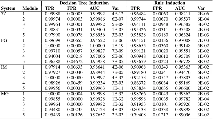
E. Restricted SimBF Fault Model

Having demonstrated the set of fault injections associated with BF is accounted for under SimBF, it is reasonable that SimBF could be used in fault injection analysis, not least with regard to the transient and permanent hardware faults that BF is commonly used to emulate. However, the computational expense of performing bit flip fault injection on exhaustive combinations of bits in each variable representation makes the model impractical for many software validation processes.

The problem of impractical experimental cost can be solved by restricting the number of fault injections performed or developing a strategy to intelligently sample the error space. To this point simultaneous bit flip fault injections have been

exhaustive. That is, ifnvariables were in scope then the fault

model was exhaustively applied to the representation of every

k-combination of variables for 1 ≤ k ≤ n. By restricting

the faults injected to being in every k-combination of bits

in the representation for 1 ≤ k ≤ 2 and, similarly only

k-combinations of variables for 1 ≤ k ≤ 2, the number

of experiments is dramatically reduced whilst preserving the essence of simultaneous fault injection.

Table VII shows the performance of the generated error detection predicates when simultaneous bit flip fault injection

is restricted to every k-combination of bits in representation

for1≤k≤2andk-combinations of variables for1≤k≤2.

This reduces the number of fault injection experiments on a

single variable from n₁+ n₂

+...+ n_k

to n₁+ n₂

, where

nis the number of bits in the variable. Similarly reducing the

number of variable combinations to n₁

+ n₂ + n₃

+...+ n_k

to n₁

+ n₂

, wheren is the number of variables in scope.

The performance of the error detection predicates generated under the SimBF model with 2 or fewer simultaneous faults, shown in Table VII, is identical to the performance of the exhaustive SimBF model for all but five software modules. In each of these cases the associated error detection predicates have decreased in TPR and FPR, hence a commensurate reduction in AUC, though the impact is less severe where the error detection predicates are generated using rule induction.

The TPR, FPR and AUC values of the five impacted soft-ware modules do not revert to the efficiencies of the BF model, despite the restricted model retaining near-perfect detection capability with regard to single fault injections. This represents a further indication that the consideration of the simultaneous fault model is providing greater depth of analysis, now at a more reasonable experimental cost. It is similarly interesting to note the consistency of the AUC variance across the exhaustive and restricted models, suggesting near identical error detection predicates are being generated, despite the cross validation process excluding informative instances for evaluation.

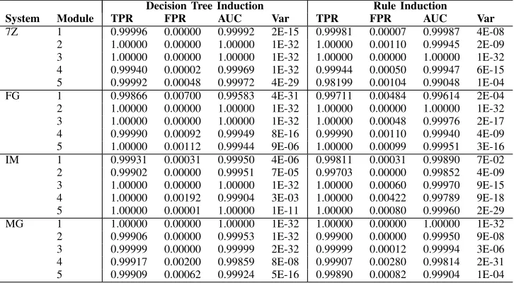
Table VIII shows the performance of the generated error detection predicates when simultaneous bit flip fault injection

is restricted to every k-combination for 1 ≤ k ≤ 3. This

increases the number of fault injection experiments conducted

for a single variable from n₁+ n₂

to n₁+ n₂

+ n₃

, wheren

is the number of bits in the representation. Similarly increasing

the number of variables combinations to n₁

+ n₂

to n₁

+ n

2

+ n₃

, where nis the number of variables in scope.

The performance of the error detection predicates generated under SimBF with three or fewer simultaneous faults, shown in Table VIII, builds on the performance of the model with two or fewer simultaneous faults. The restricted model with three or fewer simultaneous faults yields identical performance to the exhaustive SimBF fault model for all but two software modules, where these are limited to a single software system. The results presented demonstrate that the Restricted SimBF model provides a practical simultaneous fault model for the generation of efficient EDMs based on the application of machine learning to software fault injection data sets. The efficiencies of the generated error detection predicates surpass those of predicates generated under the BF model when evaluated again non-simultaneous or simultaneous faults. It should be noted that the results presented were derived under synthetic workloads and simultaneous fault models developed by existing research, a common limitation of work in the design of error and anomaly detection approaches.

VII. CONCLUSION

In this section the contributions of this paper are summarised and future work discussed.

A. Summary

(11)

[image:11.612.126.489.72.272.2]

TABLE VI: The efficiency of error detection predicates generated under the SimBF fault model and evaluated against BF data.

7Z 1 0.99996 0.00000 0.99992 2E-15 0.99981 0.00007 0.99987 4E-08

2 1.00000 0.00000 1.00000 1E-32 1.00000 0.00110 0.99945 2E-09

3 1.00000 0.00000 1.00000 1E-32 1.00000 0.00000 1.00000 1E-32

4 0.99940 0.00002 0.99969 1E-32 0.99944 0.00050 0.99947 6E-15

5 0.99992 0.00048 0.99972 4E-29 0.98199 0.00104 0.99048 1E-04

FG 1 0.99866 0.00700 0.99583 4E-31 0.99711 0.00484 0.99614 2E-04

2 1.00000 0.00000 1.00000 1E-32 1.00000 0.00000 1.00000 1E-32

3 1.00000 0.00000 1.00000 1E-32 1.00000 0.00048 0.99976 2E-17

4 0.99990 0.00092 0.99949 8E-16 0.99990 0.00110 0.99940 4E-09

5 1.00000 0.00112 0.99944 9E-06 1.00000 0.00099 0.99951 3E-16

IM 1 0.99931 0.00031 0.99950 4E-06 0.99811 0.00031 0.99890 7E-02

2 0.99902 0.00000 0.99951 7E-05 0.99703 0.00000 0.99852 4E-09

3 1.00000 0.00000 1.00000 1E-32 1.00000 0.00060 0.99970 9E-15

4 1.00000 0.00192 0.99904 3E-03 1.00000 0.00422 0.99789 9E-18

5 1.00000 0.00001 1.00000 1E-11 1.00000 0.00080 0.99960 2E-29

MG 1 1.00000 0.00000 1.00000 1E-32 1.00000 0.00000 1.00000 1E-32

2 0.99906 0.00000 0.99953 1E-32 0.99900 0.00000 0.99950 9E-08

3 0.99999 0.00000 0.99999 2E-32 0.99999 0.00012 0.99994 3E-06

4 0.99917 0.00200 0.99859 8E-08 0.99907 0.00280 0.99814 2E-31

5 0.99909 0.00062 0.99924 5E-16 0.99890 0.00082 0.99904 1E-04

TABLE VII: The efficiency of error detection predicates generated and evaluated under the SimBF fault model with simultaneous

fault injections restricted to k-combinations of bits in representation and variables for1≤k≤2.

7Z 1 0.99988 0.00005 0.99992 2E-14 0.96484 0.00063 0.98211 2E-02

2 1.00000 0.00000 1.00000 1E-19 0.98655 0.00360 0.99148 5E-02

3 0.99710 0.00057 0.99827 7E-09 0.99121 0.00020 0.99551 3E-02

4 0.96205 0.00170 0.98018 8E-06 0.94901 0.00311 0.97295 7E-03

5 0.97990 0.00078 0.98956 3E-03 0.95828 0.03180 0.96324 1E-03

FG 1 0.88218 0.00855 0.93682 1E-06 0.94151 0.00136 0.97008 7E-03

2 1.00000 0.00000 1.00000 1E-19 0.98655 0.00360 0.99148 5E-02

3 0.99710 0.00057 0.99827 7E-09 0.99121 0.00020 0.99551 3E-02

4 0.94004 0.00218 0.97006 4E-03 0.90948 0.00610 0.95709 8E-03

5 0.96588 0.04672 0.95958 7E-05 0.93679 0.00224 0.96728 8E-02

IM 1 0.97914 0.00633 0.98641 4E-06 0.90968 0.00243 0.95363 9E-02

2 0.97927 0.00040 0.98944 7E-05 0.89180 0.00241 0.94470 6E-02

3 1.00000 0.00080 0.99997 4E-32 0.92153 0.00547 0.95803 3E-02

4 0.98926 0.00459 0.99234 3E-03 0.86372 0.08034 0.89169 9E-03

5 0.99956 0.00031 0.99963 1E-11 0.93834 0.00635 0.96600 2E-02

MG 1 1.00000 0.00004 0.99998 1E-32 0.98766 0.00043 0.99362 2E-03

2 0.99855 0.00000 0.99928 1E-32 0.99598 0.00035 0.99782 9E-04

3 0.99964 0.00000 0.99982 1E-32 0.91953 0.00101 0.95926 3E-02

4 0.92249 0.00238 0.96006 5E-02 0.80100 0.00348 0.89876 8E-02

5 0.90100 0.00157 0.97657 2E-03 0.79408 0.01217 0.89096 3E-02

using fault data collected under models accounting for the oc-currence of simultaneous faults, (ii) exhaustive fault injection under a simultaneous bit flip model can yield improvements to EDM efficiency, and (iii) exhaustive fault injection under a simultaneous bit flip model can made non-exhaustive, thereby reducing the resource costs of experimentation to practicable levels, without sacrificing the efficiency of the resultant EDMs.

B. Future Work

The results presented have motivated further consideration of simultaneous fault model representativeness. The examination of fault injection data and efficient error detection predicates is a means for gaining insight into fault model representativeness. In contrast, the task of sampling error states and test cases to reduce experimental cost is well researched. Despite this, existing methods for error state and test case sampling require

domain knowledge. Examining the software states captured by efficient error detection predicates will provide insight into how to better sample error spaces and test cases.

VIII. ACKNOWLEDGEMENTS

This work was supported by The Alan Turing Institute under the EPSRC grant EP/N510129/1.

REFERENCES

[1] A. Arora and S. S. Kulkarni, “Detectors and correctors: A theory of

fault-tolerance components,” inProceedings of the 18th IEEE

Interna-tional Conference on Distributed Computing Systems. Amsterdam, Netherlands: IEEE Computer Society, May 1998, pp. 436–443. [2] M. Hsueh, T. K. Tsai, and R. K. Iyer, “Fault injection techniques and

tools,”IEEE Computer, vol. 30, no. 4, pp. 75–82, April 1997.

[3] D. Powell, E. Martins, J. Arlat, and Y. Crouzet, “Estimators for fault

tol-erance coverage evaluation,”IEEE Transactions on Computers, vol. 44,

[image:11.612.127.488.314.516.2]

(12)

[image:12.612.128.489.83.285.2]

TABLE VIII: The efficiency of error detection predicates generated and evaluated under the SimBF fault model with

simultaneous fault injections restricted to k-combinations of bits in representation and variables for 1≤k≤3.

7Z 1 0.99988 0.00005 0.99992 4E-12 0.96484 0.00063 0.98211 2E-06

2 0.99974 0.00003 0.99986 6E-07 0.99744 0.00670 0.99537 6E-04

3 0.99964 0.00001 0.99982 5E-08 0.94111 0.00948 0.96582 3E-02

4 0.98831 0.00031 0.99400 1E-05 0.95326 0.00311 0.97508 2E-03

5 0.97990 0.00078 0.98956 3E-03 0.95828 0.03180 0.96324 1E-03

FG 1 0.89699 0.00655 0.94522 1E-06 0.94151 0.00136 0.97008 7E-03

2 1.00000 0.00000 1.00000 1E-19 0.98655 0.00360 0.99148 5E-02

3 0.99710 0.00057 0.99827 7E-09 0.99121 0.00020 0.99551 3E-02

4 0.94004 0.00218 0.97006 5E-06 0.90948 0.00610 0.95709 1E-03