An algebraic characterisation of staged trees : their geometry and causal implications

warwick.ac.uk/lib-publications

A Thesis Submitted for the Degree of PhD at the University of Warwick

Permanent WRAP URL:

http://wrap.warwick.ac.uk/91331

Copyright and reuse:

This thesis is made available online and is protected by original copyright.

Please scroll down to view the document itself.

Please refer to the repository record for this item for information to help you to cite it.

Our policy information is available from the repository home page.

An algebraic characterisation of staged trees:

their geometry and causal implications

Christiane Görgen

Submitted in partial fulfilment of the requirements

for the degree of

Doctor of Philosophy

12th April 2017

Introduction 1

1. Fundamentals 9

1.1. Parametric statistical models . . . 9

1.2. Tree models . . . 14

1.2.1. Probability trees . . . 14

1.2.2. Bayesian networks as probability trees . . . 20

1.2.3. Staged trees . . . 24

1.2.4. Chain event graphs . . . 30

1.3. Algebraic Statistics . . . 33

1.3.1. A very abbreviated introduction to algebraic geometry . . . 34

1.3.2. Algebraic notions for staged trees . . . 37

2. A geometric analysis of staged tree models 43 2.1. A characterisation in terms of odds ratios . . . 44

2.2. Staged trees as algebraic statistical models . . . 53

2.3. All staged tree models on four atoms . . . 62

3. The interpolating polynomial 71 3.1. A differential approach . . . 73

3.2. Polynomial and statistical equivalence . . . 80

3.2.1. The swap operator . . . 82

3.2.2. The resize operator . . . 98

3.2.3. The full statistical equivalence class . . . 103

3.2.4. The Christchurch Health and Development Study (CHDS) . . . 104

3.3. Eliciting a graph from a tree-compatible polynomial . . . 109

4. Causal inference in staged tree models 119 4.1. Causal interventions on staged trees . . . 120

Conclusions 133

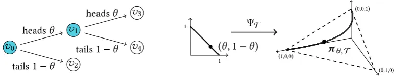
0.1. A staged tree model on three atoms. Graphical representation in terms of a col-oured probability tree and depiction as a parametric curve inside a probability

simplex. . . 2

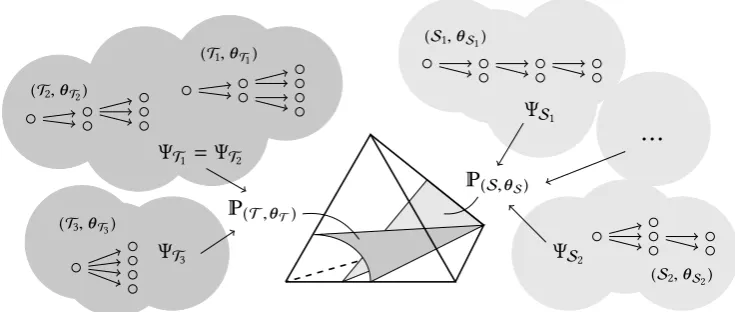
0.2. An illustration of the different aspects of probability tree models analysed in this thesis. . . 4

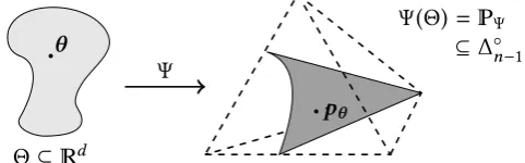
1.1. A discrete and parametric statistical model. . . 11

1.2. An event tree graph. . . 16

1.3. An acyclic digraph which can be transformed into anX-compatible tree. . . . 23

1.4. Two graphical representations for the biology model in Example 1.12. . . 27

1.5. A stratified staged tree, simplified version taken from Barclay et al. (2013). . . 30

1.6. A chain event graph. . . 33

2.1. Primitive probabilities are fractions of probabilities of vertex-centred events. . 45

2.2. Two probability trees whose stage structure is captured in form of polynomial equations in Examples 2.3 and 2.8. . . 47

2.3. An illustration of the solution sets characterised in Lemma 2.5. . . 50

2.4. The image of a tree parametrisation is not necessarily contained in the prob-ability simplex if constraints on its domain are relaxed. . . 60

2.5. All staged trees with four root-to-leaf paths. . . 63

2.6. All staged tree models on four atoms. . . 67

2.7. The varietyV(π3π1−π2(π1+π2)) _⊆’3contains the staged tree model (2.40.6). 69 3.1. An arithmetic circuit for computing an interpolating polynomial. . . 79

3.2. Two polynomially equivalent staged trees with twins and a swap. . . 86

3.3. Three polynomially equivalent labelled event trees. . . 91

3.4. Junction tree representations for Example 3.29. . . 95

3.5. Two staged trees polynomially equivalent to the one in Fig. 1.5. . . 97

3.6. A resize of a star into a binary tree. . . 100

3.8. Three polynomially equivalent staged trees for the CHDS dataset. . . 107

3.9. A root-to-leaf pathλ=(e₁, . . . ,e_l)in an event tree. . . 112

4.1. Two graphical representations for a causal manipulation. . . 123

4.2. A staged tree polynomially equivalent to the one from Fig. 4.1.1. . . 125

4.3. Two alternative graphical representations for a local manipulation. . . 128

First and foremost, I am immensely grateful to my supervisor Jim Smith for the excellent guid-ance and support. Jim has been an exceptional teacher, supervisor and collaborator who has always been available and has never ceased to encourage my efforts. His personal enthusiasm and his scientific intuition have provided me with the best start to an academic career I could have wished for.

Further major thanks go to four people who have played a central role in my young academic life: to my Italian collaborators, Manuelle Leonelli, Eva Riccomagno and Anna Bigatti, for being amazing people to work with and to Elke Thönnes for being a role model.

Second, I wish to thank the panel of my interim reports, Jon Warren and Wilfrid Kendall, for their very thorough examination of my work. The suggestions I have received from both professors have been hugely helpful in improving the presentation of my results.

I declare that I have developed and written the enclosed thesis completely by myself and have not used sources or means without declaration in the text.

I am first author of two papers. The first paper is entitledEquivalence Classes of Staged Trees,

throughout cited as Görgen and Smith (2015), and has been developed in close collaboration with my supervisor Jim Smith. This paper forms the core of my project and has been accepted subject to minor revisions by Bernoulli. An extended version of the results of this paper— containing a number of new examples and additional insights—is the content of Section 3.2 (Polynomial and statistical equivalence) of this thesis. The second paper, entitledA differential approach to causality in staged treesis here cited as Görgen and Smith (2016) and has been

de-veloped in an equally close collaboration. This work was accepted to the proceedings of the Eighth International Conference on Probabilistic Graphical Models after successfully complet-ing a double-blind peer-review. The material of that paper forms Section 4.1 (Causal interven-tions on staged trees) of this thesis. In both of these publicainterven-tions, I have lead the preparation of the material and the conceptual work.

I am joint first author ofA Differential Approach for Staged Trees, cited as Görgen et al. (2015).

This paper has been published in the conference proceedings of the European Conference on Symbolic and Quantitative Approaches to Reasoning with Uncertainty after peer-revision. All material herein has been developed jointly with Manuele Leonelli, with Jim Smith taking a supervisory role, and has my co-author’s approval for presentation in this thesis. These results can be found in Section 3.1 (A differential approach). In addition, the preprint entitled Sensit-ivity analysis, multilinearity and beyondand cited as Leonelli et al. (2015) contains joint work

with Manuele Leonelli and Jim Smith that I am not the lead author of. In this thesis, I will refer to that paper exclusively for pointing out related streams of research, without repeating any of the original results.

The report entitledDiscovering statistical equivalence classes of discrete statistical models using computer algebrais here cited as Görgen et al. (2017) and is the result of joint work with Jim

tree-compatible polynomial) and I have my collaborators’ approval for doing so.

Finally, I am one of three authors of the bookChain Event Graphs, here Smith et al. (2017),

which is currently in preparation for Chapman and Hall. The three chapters I am mainly responsible for contain both new material and parts of the material cited above as well as supplementary illustrations which are not additionally published in this thesis. Chapters in that book which have been written by my co-authors are not repeated in this thesis, and relevant results which are cited here are always marked by their original source.

Chapter 1 (Fundamentals) and Chapter 2 (A geometric analysis of staged tree models) as well as Section 4.2 (Causal discovery in the CHDS) have at the time of writing not been pub-lished elsewhere. In particular, the material presented in Chapter 2 is entirely my own work and I am currently preparing these ideas for a collaboration with Piotr Zwiernik from the Uni-versitat Pompeu Fabra, Spain. The two new streams of research—algebraic geometry and causal discovery—that are only touched upon in these chapters form the foundational part of work in progress which will be discussed at the very end of this thesis.

This text has been typeset using the KOMA-Script classscrbookof LATEX2_ϵ. All illustrations except for Figs. 2.6 and 2.7 have been created using thetikzandpgfplotspackages (pgf TikZ,

Probability trees—or tree diagrams—are perhaps best known as useful illustrations for solving problems in high-school mathematics. For many students, these trees may be the first type of ‘graphical model’ to come across, and even in undergraduate probability classes a quickly drawn tree graph can help to solve tricky questions (Blitzstein and Hwang, 2014). Typical ap-plications of probability trees include discrete experiments such as coin tossing: illustrated in Fig. 0.1. Here, the likelihood of an outcome of the experiment can simply be calculated by multiplying transition probabilities along the relevant path in the tree and possibly summing over all paths belonging to an event of interest. Despite this common application in not too advanced mathematics, the usefulness and true value of probability trees in statistical infer-ence has, until recently, not been fully appreciated by the scientific community. Although tree graphs are frequently used in decision analysis, probability trees themselves have had consid-erably less interest and the standard theory of graphical models is very much dominated by Bayesian networks. In fact, it was Smith and Anderson (2008) who first successfully estab-lished a statistical framework for using probability trees as more than pretty illustrations of simple problems: the authors developed statistical methodologies based on the properties of probability trees which could be applied to inference for instance in health and social sciences. Their main contribution was to establish an elegant and self-contained toolbox to use prob-ability trees not for embellishing other statistical models but as graphical statistical models in their own right. Now, eight years on, researchers have understood this framework so well and have used it so successfully that we are ready to go one step further. We can now use only the abstract characterisation of a model represented by a probability tree and develop statistical methods based on this, without explicitly referring back to a tree graph. In doing so, we are able to find surprising analytical results in a very general framework.

v₀

v1

v2

v₃

v₄

headsθ

tails1₋θ

headsθ

tails1₋θ

(0.1.1)A probability tree (T,θ_T) which represents a repeated coin-toss model.

1

1

(θ,1₋θ) Ψ_T

•_π θ,T (1,0,0)

(0,1,0) (0,0,1)

(0.1.2)The parametrisationΨ_T belonging to(T,θ_T)from Fig. 0.1.1 maps edge labels to a point in the model (0.1). Figure 0.1.A staged tree model on three atoms. Graphical representation in terms of a coloured probability tree and depiction as a parametric curve inside a probability simplex.

order to improve current model selection techniques. And fourth, to develop a framework in which probability trees can be given a putative causal interpretation.

The very simple example below illustrates some of the key ideas of this thesis.

Consider a coin toss which will be repeated once if the first outcome is heads. The probability of heads is assumed to be strictly positive but unknown. We can draw a probability tree denoted

(_T,θT)and depicted in Fig. 0.1.1 to represent this problem. The pair (T,θT)is then given by a tree graph_T, illustrating how the experiment unfolds, and a vector of labelsθ_T whose

components are conditional probabilities of events. In our example, the graph _T = (V,E)

has a vertex setV = {v₀,v₁,v₂,v₃,v_4} and an edge setE = {e₁ = (v₀,v₁),e₂ = (v₀,v₂),e₃ =

(v₁,v₃),e₄ = (v₁,v₄)_{} ⊆} V _×V. We label the edgee₁by the probability of heads, denoted θ = θ(e1), and, because the transition probabilities from the same vertex shall sum to unity,

the edgee₂by the probability of tails, soθ(e₂) = 1−θ. Because two tosses of the same coin

are independent, the transition probabilities fromv₀ to v₁ andv₂ are the same as fromv₁

tov3 andv4, or rather θ(e3) = θ(e1) andθ(e4) = θ(e2). We always code these equations

graphically by assigning the same colour to those vertices in the graph which have the same emanating edge labels: here, using blue colour in Fig. 0.1.1. Two equally coloured vertices are said to be in the samestage. The vector of labelsθT = (θ(e1),θ(e2)) of this probability

tree lies inside the parameter space depicted on the left hand side of Fig. 0.1.2. Note that we will often over-parametrise a model in the way we do here. This approach will be particularly useful when subsequently ignoring sum-to-1 conditions. Now, the set of root-to-leaf paths

Λ(_T) = {λ₁,λ₂,λ_3}of the probability tree corresponds to the set of possible single outcomes

of our experiment as follows. We identify the sequence of edgesλ1= (e1,e3)with the outcome

‘heads, heads’,λ2=(e1,e4)with ‘heads, tails’ andλ3= (e2)with ‘tails’. When multiplying edge

labels along these paths, we obtain the probabilities of the respective outcomes asπ_θ,T(λ1)=

fulfil the criteria above, for all possible probabilitiesθ of ‘heads’:

(T,θ_T) =

θ2,θ(1₋θ),1₋θ _|θ _∈(0,1). (0.1)

Note that all components of a vectorπθ,T ∈(T,θ_T)in the model are strictly positive and sum to unity, and that every vector thus corresponds to a positive distribution over the three atoms. The set (0.1) of all these distributions is called a probability tree model. The model (T,θ_T)can be defined as the image of a bijective map

Ψ_T : ((θ1,θ2)_∈(0,1)2_|θ1+θ2=1)→(T,θ_T), (θ,1−θ) 7→πθ,T (0.2)

which identifies a choice of parameters with a vector of atomic probabilities. Every probability tree thus specifies a parametrisation rule whose image is the model represented by that tree. The probability tree itself is a graphical representation of that model. Interestingly, the map (0.2) also determines a parametric curve in three-dimensional space. We draw this curve, and thus the model(T,θ_T)from (0.1), inside a two-dimensional (probability) simplex on the right hand side of Fig. 0.1.2.

So instead of limiting ourselves to using the probability tree merely as an elegant picture of a discrete experiment, we have already found three different viewpoints from which to analyse this example setting. First, we can characterise properties of the pair (_T,θT) as a labelled graph in the framework of graph theory and computer science. Second, we can specify a prob-ability tree model(T,θ_T) as the set of probability distributions represented by such a graph

(_T,θT). Third, we can define this model as the image of a certain bijective mapΨT. The role played by the labels of a probability tree then changes according to the framework we choose: every component of a vectorθ_T is simply a label in a symbolic framework—or an indetermin-atein an algebraic framework—but aparameterin a geometric and aprobabilityin a statistical framework. We unravel this subtlety in the first chapter below. Within this text, we will then combine all of these different viewpoints, and thus three usually thought of as different discip-lines of mathematics, to answer some simple questions in probability tree models. In addition to the individual results achieved and presented below, in this thesis we thus also make a major contribution in linking the relatively recent study of coloured probability trees to well-known concepts across other fields of research.

(S,θ_S)

_(T,θT)

Ψ_T1 = Ψ_T2

Ψ_T3

Ψ_S1

Ψ_S2

...

(T1,θ_T1) (T2,θ_T2)

(T3,θ_T3)

(S1,θ_S1)

(S2,θ_S2)

Figure 0.2.An illustration of the different aspects of probability tree models analysed in this thesis.

light and dark grey inside this space depict two different generic tree models: as sets of points, or parametric curves, just like in the example above. These models can be specified as the im-ages of feasible parametrisations. Each such parametrisation is in turn induced by a collection of probability tree representations, depicted inside their respective cloudy shapes. The four chapters of this thesis will each analyse a different component of this picture: Chapter 1 form-ally defines all objects within the figure, Chapter 2 analyses algebro-geometric properties of the hypersurfaces inside the simplex, Chapter 3 characterises all probability trees which share a common parametrisation map and all parametrisations which induce the same model, and finally Chapter 4 abstracts from this picture to give a probability tree model an interpretation in an inferential context of interest. In particular, the content of these chapters is as outlined below.

In Chapter 1 of this text we introduce the probability tree model as a certain type of dis-crete statistical model and embed it in well-established theory of statistical methodology and Algebraic Statistics. We show how this formalism significantly tightens the initial work on probability trees. Staged treeandChain Event Graph (CEG) models were first designed to

de-scribe discrete processes which do not follow the implicit symmetries in Bayesian network (or often for shortBN) models. It was only later appreciated how important this class was in

algorithms and model selection techniques. We repeat the respective definitions and give an overview of the relevant results in the main body of the text.

Whilst early publications in this field used the terminology ‘staged tree’ and ‘staged tree model’ exchangeably, we now appreciate the necessity to distinguish between a graphical rep-resentationof a statistical model and the model itself, which is a collection of probability

distri-butions with certain properties. This distinction is common practice in the theory of Bayesian networks whereacyclic digraphsorMarkov random fieldsare graph representations of an

un-derlying statistical model (Lauritzen, 1996). These representations code conditional independ-ence assumptions between a set of random variables in a network where problem variables are vertices and the absence of edges between vertices indicates (conditional) independence assumptions. The set of all distributions which respect these assumptions then determines the corresponding statistical model, a Bayesian network model. We show that every discrete BN model can be represented by a staged tree or CEG but that in many problems CEGs are much more expressive.

In Chapter 2, we make first advances in an analysis of the geometric properties of staged tree models. Here, we always specify such a model as the image of a parametrisation map. For instance in the toy example above, this image was simply given by a parametric curve. In much more generality, staged tree models can be equivalently characterised as solution sets of systems of very specific polynomial equations. Ours models are hence algebraicvarieties or

rathersemi-algebraic sets when imposing positivity constraints on the immanent probability distributions. The main purpose of this chapter is to infer the nature of the equations defining these sets and to present a number of small-scale examples. Intriguingly, we find in Theorem 1 that the system of equations characterising the stage structures in a coloured probability tree always corresponds to relationships betweenodds ratiosof probabilities of events. These

equa-tions allow thus for a very straightforward interpretation in terms of the underlying statistical model. Just like a coloured identification of edge labels in a staged tree, these odds-ratio equa-tions can also be simply read from a tree graph.

We then present a complete analysis of all staged tree models on three or four atoms, drawing these as subsets of probability simplices: compare Figs. 0.1 and 0.2 above. Throughout this chapter, we list methods from algebraic geometry which can be employed in this type of study of a statistical model and outline the challenges which arise when analysing a probabilistic object within an algebraic framework.

this end we define two staged trees to bestatistically equivalentif and only if they represent the same probability tree model—so if they are in a cloud of the same colour as the corresponding surface in Fig. 0.2. We will then solve two problems which are central to statistical inference:

1. How can we classify all staged trees representing the same model?

2. Are every two members within a class of statistically equivalent model representations connected by simple ‘local’ operations?

Thwaites and Smith (2015b) have shown that the question of statistical equivalence in staged tree models can unfortunately not be answered in a purely graphical fashion, as is the case in BN models. However, using the machinery developed in Chapter 1 and Görgen and Smith (2015), we will show that every probability tree is in one-to-one correspondence with a certain factorisation of a polynomial in the edge labels of that graph. We call this polynomial the

interpolating polynomialand derive that all graphs belonging to the same model then share that

same interpolating polynomial, up to possible reparametrisations. Those that share a common polynomial description are in the same cloudy shape in Fig. 0.2 while those that need to be reparametrised are in different clouds pointing towards the same hypersurface in that figure. This answers question (1.) above. Interestingly, the interpolating polynomial can then also be used to answer question (2.). In fact, an application of the distributive law on a certain ‘nested’ form of an interpolating polynomial corresponds to a local change of a subgraph in the staged tree. A series of reorganisations of the nesting together with substitutions of factors in the polynomial is then shown to be analogous to what we callswapandresize operations in the graph. That these can traverse the full equivalence class is the key result of Theorem 2.

We conclude this development with an application of the swap and resize operators on the statistical equivalence class of a staged tree fitted to a real dataset.

In the same chapter, we find a number of other useful features of the interpolating poly-nomial. These are its use in calculating marginal and conditional probabilities in staged tree models using a differential operator as developed in Görgen et al. (2015) and its role in an al-gorithmic elicitation of all members in a given equivalence class of staged trees using computer algebra as in Görgen et al. (2017).

which events can be depicted across a statistical equivalence class. So following Pearl (2000) we assert that if there are two graphical model representations, one stating that an eventA

can happen before a different eventB and the other representation reversing that order toB

happening beforeA, then we would not want to considerAas a possible cause of B or vice

versa. However, if there is an unambiguous ordering across all possible staged tree represent-ations, then we might call one event aputative causeof the other and employ causal inference techniques to measure the strength of that causal effect. We show how this notion can be formalised for staged trees.

In this first chapter we will start off by introducing very general probability trees. These trees can provide elegant graphical representations of certain parametric statistical models. In par-ticular, via a colouring of their vertices, they can code a number of conditional independence assumptions: a tool frequently used in describing real systems. We illustrate briefly that such coloured probability trees—calledstagedtrees—can be specified either by imposing linear con-straints on their parameter space or by finding polynomial concon-straints on certain probabilities of events in an underlying space. Deferring a deeper analysis of this observation to the sub-sequent chapter, we then show that every discrete Bayesian network model can be represented by a staged tree. A small-scale example simplifying a real system illustrates this point. We explain why a graphical representation in terms of a probability tree can often be much more expressive than the more standard choice of an acyclic digraph. We then end the chapter in-troducing some vocabulary from algebraic geometry and polynomial algebra which can be naturally used to capture properties of staged trees. A translation of notions from algebra to staged trees and back will be central to the development in this thesis.

Throughout, we assume a basic knowledge of Bayesian networks (BNs) in order to be able to compare our new tools with those which are well known in graphical models. The terminology

Bayesian network model—or for short BN model—hereby refers to a set of probability

distribu-tions with certain features, and the termacyclic digraphrefers to a graphical representation of

that set, given by a directed graph with no directed cycles. All further concepts needed will be very briefly repeated below. A thorough introduction to BN models can be found in Lauritzen (1996) and a more applied approach is presented for instance in Smith (2010).

1.1. Parametric statistical models

A statistical model, as defined below, is simply a set of probability distributions over a given space (Blitzstein and Hwang, 2014). If that space is countable, we say that such a model is

discrete. Every distribution in a finite and discrete statistical model can be specified as the

Following Drton et al. (2009), discrete statistical models are thus sets of vectors with the above property, so sets of points lying inside aprobability simplex

∆_n−1= (p _∈’n _|

n

X

i=1

p_i =1, and 0_≤p_{i ≤}1 for alli=1, . . . ,n) (1.1)

wheren _∈ Ž is the cardinality of the discrete space. When distributions are assumed to be strictly positive, they are elements of the open probability simplex ∆◦_{n−1 ⊆} ∆n−1 where p_{i ∈}(0,1)for alli=1, . . . ,n. For the purpose of this thesis we often assume openness of

prob-ability simplices. This assumption enables us to avoid distracting technical issues concerning boundary cases and so to focus more directly on inferential matters.

Statistical models can often be characterised using a set of parameters and may then be defined as families of distributions together with certain constraints on these parameters, for instance constraints on the mean and the variance in Gaussian models. Whenever this is the case it is vital to be able to uniquely identify each parameter in a space with one distribution in the model. We will thus use the following definition:

Definition 1.1(Parametric statistical model). LetΩ always denote a finite space withn _≥ 2

atomsω _∈Ω, and letΘ _⊆ ’d,d _∈Ž, denote a parameter space. We writepθ :Ω →(0,1)for

a strictly positive probability mass function over the atoms of such a finite space, and always assume thatpθ can be parametrised using someθ ∈ Θ. The vector of values of that function

is denoted by the bold characterpθ =

pθ(ω) | ω ∈ Ω

. Henceforth we call each of the componentspθ(ω),ω ∈Ω, of that vector anatomic probability.

Adiscrete parametric statistical modelonΩis a set of vectors as above

Ψ=

(

p_{θ |}θ _∈Θ)_⊆ ∆◦_n−1 (1.2)

which lie in the openn₋1-dimensional probability simplex (1.1) forn = #Ω. The indexΨin

Ψis a bijective map

Ψ: Θ_→Ψ, θ 7→pθ (1.3)

which uniquely identifies a choice of parameters with a distribution in the model. Ψis called

aparametrisationof the modelΨ =Ψ(Θ).

θ

Θ _⊆’d

Ψ

pθ

Ψ(Θ) =Ψ ⊆ ∆_n◦₋₁

Figure 1.1.A discrete and parametric statistical modelΨ = Ψ(Θ)depicted in dark grey as a subset of then₋1-dimensional open probability simplex∆_n◦₋₁, here illustrated as the hatched

tetrahedron. The model equals the image of a parametrisationΨ : Θ _→ ∆◦_n−1,θ 7→pθ with

parameter spaceΘ _⊆’d depicted in light grey.

the model itself. Also note in this context that we use the blackboard bold letterfor sets of probability distributionsp, rather than for a probability measure—here instead denotedP—as

is often the case in the literature. Bold symbols such asporθ always indicate vectors, and

calligraphic symbols will be reserved for graphs.

We will henceforth restrict our analysis to discrete models which can always be paramet-rised. So we always refer to a discrete and parametric statistical model when using the term ‘model’.

In the symbolic and algebraic framework used in later sections, instead of specifying a para-meter space Θ _⊆ ’d we will often interpret a parametric model as a set of points whose components can be expressed usingindeterminatesθ = (θ₁, . . . ,θ_d). We would then choose

one symbolic vectorp_θ to represent a set {p_θ | θ ∈ Θ_}. For instance, in the example from

page 2 this would amount to representing the coin-toss model by a vectorp_θ = (θ₁2,θ₁θ₂,θ₂)

whose components are products of indeterminatesθ = (θ₁,θ₂)instead of substituting values

such that these indeterminates are probabilities,(θ1,θ2)_∈∆◦_2−1⊆ ’2.

The discipline of Algebraic Statistics has successfully followed such a symbolic approach to inference and has used it to analyse the algebraic and geometric properties of a number of interesting statistical models, mostly discrete or Gaussian: see the detailed discussion in Chapter 2. In this development, a statistical model is often characterised using polynomial equalities (and inequalities) of one of two types. The first type constrains atomic probabilities, so here we would have a collection of fi(p) = 0 where a probability distributionp ∈∆n−1

functions as a vector of indeterminates andf_iis a polynomial for alli =1, . . . ,k. Alternatively,

constraints to be of polynomial form, model parametrisations are often assumed to be rational functions. In the type of models we introduce below, sometimes polynomial constraints on atomic probabilities can be equivalently expressed as polynomial constraints on parameters and vice versa:

Definition 1.2(Monomial parametrisation). LetΨbe a parametric model as in Definition 1.1. We say that the mapΨ:Θ_→Ψis amonomial parametrisationif every component of its image is a monomial

Ψ_i(θ)=θαi,1

1 · · ·θdαi,d (1.4)

in the parametersθ =(θ1, . . . ,θd)∈Θwith non-negative exponentαi =(αi,1, . . . ,αi,d) ∈šd_≥0 fori=1, . . . ,nandd _∈Ž. A monomial parametrisation is calledmultilinearif the multiplicity of every parameter in every such monomial is at most one,α_{i ∈ {}0,1_}d for alli =1, . . . ,n. We

then also call the modelΨamultilinear model.

A monomial expression like (1.4) is often called apower product(Pistone et al., 2001a) in

Al-gebraic Statistics: see Section 1.3. Perhaps more familiar to the reader than the power-product representation of a monomial model is its alternative reparametrised form as an exponential family

Ψ_i(ϕ)=exp*

,

d

X

j=1

α_i,jϕj+

- (1.5)

whose parametersϕ = (ϕ1, . . . ,ϕd) are given byϕj = log(θj) andθj ∈ (0,1), j = 1, . . . ,d. Incidentally, because of this equivalence the tree models we define in the next section can be viewed as exponential families or log-linear models. In this thesis we will usually prefer the expression (1.4)—which further enables us to interpret multilinear models as certain families of multinomial distributions—over (1.5). This is in order to avoid having to deal with positivity conditions of parameters and in order to be able to develop a theory which links the edge labels of a graph directly to a polynomial representation. This theory in turn has then some surprisingly natural links to other areas of mathematics as we will point out in the introduction to Chapter 3.

Monomial parametrisations commonly occur in statistical modelling. For instance, in every Bayesian network model atomic probabilities are of the typepθ(ωi) = θ₁αi,1· · ·θ_dαi,d where

i = 1, . . . ,n. In this case, theθ-parameters are conditional or marginal probabilities: see also

Consider now an example of a multilinear model which can be completely characterised by a collection of very special polynomial constraints.

Example 1.3(Cross-product differences). We briefly recall a setting analysed in Geiger et al. (2006). LetΩbe a discrete space and letX = (X1,X2,X3) : Ω _{→ {}0,1_}3be a vector of random variables measurable with respect to that space, with a strictly positive probability distribu-tionp : _{0,1_}3 _→ (0,1). We denote the values taken by that distribution by the shorthand px1x2x3 =p(x1,x2,x3)using subscripts for function argumentsxi = 0,1 andi = 1,2,3; and we denote the corresponding vector of atomic probabilities byp= (p_{x1x2x3 |}x_i = 0,1, i=1,2,3).

This vector is an element of the open seven-dimensional probability simplex,p ∈∆◦₈₋₁, because

its eight entries sum to one and are positive. It is easy to check1_{that a statement of the type}

‘X₁is independent ofX₃givenX₂’—in symbolsX_1⊥⊥X_3|X₂—translates into what the authors

of the publication cited above callcross-product differenceson the atomic probabilities. These

are polynomial constraints of the form

f₁(p)=p₀₀₀p₁₀₁₋p₀₀₁p₁₀₀=0 and f₂(p)=p₀₁₀p₁₁₁₋p₀₁₁p₁₁₀=0. (1.6)

So the discrete conditional-independence model we analyse here can be specified as the intersection of the set of all points which both fulfil (1.6) and also lie within a probability simplex:

=(p∈’8| f1(p) =0 and f2(p) =0)∩∆◦₈₋₁. (1.7) In the language of Chapter 2, the model thus equals the intersection of a toric variety with a linear affine hyperplane and a semi-algebraic set.

We will now show here that—different from the approach followed by the authors cited above— can equivalently be specified as a parametric model as in Definition 1.1. This is because the conditional independence constraint above can be expressed by the acyclic digraph

X1→X2→X3and we can write the distributionpx1x2x3 =θx1x2θx1x2x3 in form of a recursive factorisation according to that graph, so as the product of two parametersθ_x1x2 = p(x₁,x₂)

andθx1x2x3 = p(x3|x1,x2)which are marginal and conditional probabilities, forxi = 0,1 and

i =1,2,3. Then the conditional independence assumption above translates into the polynomial constraints

дjk(θ)=θ0jk−θ1jk =0 forj,k=0,1 (1.8)

whereθ = (θ₀₀, . . . ,θ₁₁₁). Hence, the model (1.7) is a parametric model=Ψwith multilinear parametrisation

Ψ: ∆◦_4−1×∆◦_8−1∩(θ ∈’12|дjk(θ)=0 forj,k =0,1)→∆◦8−1 (θ00,θ01,θ10,θ11,θ000,θ001, . . . ,θ111)_7→(θijθijk |i,j,k=0,1)

(1.9)

such that the image ofΨequals the model itself.

There are two important points to note here. First, the constraints in (1.6) are polynomial whereas the new constraints in (1.8) are linear. So our alternative representation is both algeb-raically and geometrically much simpler than the original cross-product differences. However, the linear constraints have the drawback that they depend on a chosen parametrisation of the model. Similarly, and second, whilst (1.9) expresses the properties of our model via a constraint on the domain of a chosen parametrisation, (1.7) expresses these equivalently as constraints on the image of that parametrisation: compare again Fig. 1.1. We will learn in Chapter 2 that in the type of models we are most interested in, linear constraints on the domain of a para-metrisation always translate into polynomial constraints on the image and that both of these characterisations are equivalent.

We will come back to the example above in subsequent sections. Despite its simplicity, it enables us both to discuss an interesting parametric model in a rigorous mathematical fash-ion with a view on possible algebraic characterisatfash-ions of the properties of the underlying probability distributions, and it can be represented by a set of probabilities trees which can be analysed using that algebraic characterisation. In fact, the for us most interesting models are those parametric models whose parametrisation can be read from a certain graph structure. These are also termedgraphical models, or here in particulartree modelsbecause the graph we are interested in is (almost) always a tree graph.

1.2. Tree models

We will firstly recall some notation in order to be able to unambiguously discuss objects from graph theory. We then define models which can be represented by certain graphs, and we formally introduce parametric statistical models with that property. Centrally, our graphs can be enhanced with an additional feature—a colour—to capture key modelling assumptions.

1.2.1. Probability trees

Definition 1.4(Event tree). A finite graph denoted_T = (V,E)with vertex setV and edge

setE _⊆V _×V is called atreeif it is connected and has no cycles. In adirectedtree, each edge

e= (v,v0) _∈Eis a pair of ordered vertices. We call vertices pa(v) = {v0 _|there is(v0,v) _∈E_}

theparentsofv _∈V and ch(v) = {v0 _∈V _|there is (v,v0) _∈ E_} the set ofchildren ofv _∈V.

A vertexv0 ∈V without parents is called aroot of the tree and vertices without children are

calledleaves. We use the symbolλ and the termroot-to-leaf path for a directed sequence of

edgesE(λ) _⊆ Ewhere one edgee = (v,v0)precedes anothere0 = (w,w0)only ifv0 =w, and

where the first edge in the sequence emanates from the root and the final edge terminates in a leaf. Asubpathin a directed tree is then a connected subsequence of a root-to-leaf path. We call

a directed tree anevent treeif all vertices except for one unique root have exactly one parent and each parent which is not a leaf has at least two children.

We denote the set of all root-to-leaf paths of an event tree byΛ(_T). The power set of the

set of root-to-leaf paths is called thepath sigma-algebraof the tree, denotedσ(_T). For fixed v _∈V ande _∈Ewe definevertex-oredge-centred eventsin the path sigma-algebra as the set of

root-to-leaf paths passing through that vertex or edge, so

Λ(v) = (λ_∈Λ(_T)_|there is an edge(_·,v) _∈E(λ)), (1.10.1)

Λ(e) = (λ_∈Λ(_T)_|e_∈E(λ)). (1.10.2)

We setΛ(v0)=Λ(_T).

A graph_T0 _{= (V}0_,E0_{) where(V}0_,E0_{) ⊆ (V,E)is called asubtree of T = (V,E) if it is an} event tree. We then write_T0 _{⊆ T. We say that a subtreeT(v) ⊆ T is aninducedsubtree if}

v _∈V and if the root-to-leaf pathsΛ(_T(v))of this subtree coincide precisely with root-to-leaf

paths in the eventΛ(v) _⊆Λ(_T)centred atv, except for the subpath fromv₀tovin the original

tree_T. We call a subtree (_{v_{} ∪}ch(v),E(v)) _{⊆ T} whose root-to-leaf paths are single edges E(v) = {(v,v0) _∈ E _|v0 _∈ ch(v)_}emanating from the same vertexv _∈V afloret, henceforth

denoted by the shorthand_Fv = (v,E(v)).

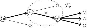
An illustration of the different concepts of the above definition is provided in Fig. 1.2. When representing a tree model as defined below, an event tree _T = (V,E) depicts all

possible unfoldings of events within a system. In particular, every root-to-leaf pathλ_∈Λ(_T)

then corresponds to an atom in an induced sample space and depicts one possible history of a unit in the system. Every vertexv _∈V denotes a state that a unit following a root-to-leaf

pathλ_∈Λ(v)might find itself in, and every edgee= (v,v0)denotes the possibility of passing

from one situationv to the nextv0. The setsΛ(v)or Λ(e), forv _∈V ande _∈ E, of all paths

v₀

v

v0 e

Fv

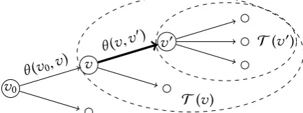
Figure 1.2.An event tree_T = (V,E)with rootv0∈V and non-leaf verticesv,v0 _∈V which

are connected by the edgee= (v,v0)_∈E. The floret_Fv is encircled. The thick depicted edges

correspond to root-to-leaf paths in the edge-centred eventΛ(e). Note that this is equal to the

vertex-centred eventΛ(v0). The induced subtree_T(v) _{⊆ T} is given by the two florets_Fv and Fv0, and the induced subtree T(v0) = Fv0 is a single floret. For simplicity, leaf vertices are

often not named.

central role in the analysis of event trees, as we will see below. Note for instance that Moivrean eventsΛ(v)are in one-to-one correspondence with induced subtrees_T(v)if we ‘condition on’

arriving at their rootv _∈ V. This graphical property is reflected in the calculation of the

probabilities of these events: see Sections 2.1 and 3.1. Naturally, root-to-leaf paths are in one-to-one correspondence with leaf-centred events. We prefer to think about these as sequences of edges because we are often interested in the entire history of a unit rather than in its final state. Furthermore, because the graphs we examine are directed, they allow for an analysis of that directionality and an induced order on vertex- or edge-centred events. So event trees are particularly expressive in terms of an ordering of events, rather than of random variables as is the case in acyclic digraphs. As Thwaites and Smith (2015b) noted, unlike for Bayesian network models, random variables are in fact rather artificial primitives to use in tree models, and alternative event-based semantics suggest themselves. We will see examples of this below and refer to Smith et al. (2017) for further details.

We have developed the following formal definition in order to enable us to equip event trees with a probability distribution.

Definition 1.5(Labelled event trees and probability trees). Let _T = (V,E) be an event tree

and assume there are labelsθ(e) =θ(v,v0)associated to all edgese= (v,v0) _∈E. We call the

vector of all labels on edges emanating from a common vertex a vector offloret labels, denoted θv = θ(e)|e∈E(v). Then the vectorθT = (θv |v ∈V)denotes all labels associated to the event tree2_{. The pair(T,θ}

T)of event tree graph together with a vector of labels is henceforth called alabelled event tree.

We will call a labelled event tree whose labels can take real values aprobability tree if all vectors of floret labels lie within probability simplices, soθv ∈ ∆◦_#E(v)−1for allv ∈V. Then

2 We usually do not a priori assume a particular order on the entries of this vector. Note also that ifvis a leaf then

the vector of all labelsθ_T is an element of a parameter space which is a product of probability

simplices, denotedΘ_T =

×

primitive probability.

Subtrees of probability trees with inherited edge labels are called(probability) subtrees.

In applications in statistical modelling, we can interpret a labelθ(v,v0) on an edgee =

(v,v0) _∈ Ein a probability tree as the transition probability of passing from a situationv to

a situationv0 along that edge in the tree. A vector of floret labelsθv can then be thought of as a vector of conditional transition probabilities. Importantly, the constraint that floret labels shall be elements of probability simplices ensures that primitive probabilities are positive and those belonging to the same floret sum to unity: soP_e∈E(v)θ(e) = 1 andθ(e) ∈ (0,1)for all non-leavesv _∈V ande _∈E.

Note that because of the interpretation above, edge labelsθ(e) were formerly denoted as

conditional probabilities πe(v0|v) (Smith and Anderson, 2008). However, within this thesis we often prefer to think of primitive probabilities as unnormalised potentials which can be marginal or conditional probabilities as in Lauritzen (1996) and whose meaning can be inferred from their positioning within a tree graph. This flexibility is key when discussing statistical equivalence in Chapter 3. Here, two probability trees representing the same model might have the same labels but their respective interpretation—and floret sum-to-1 conditions—can be very different.

Labelled event trees will be important later in this text when we interpret the labels of an event tree simply as indeterminates which are unknown, or not assigned any values. We can then determine whether such a labelled event tree can in fact be a probability tree (Chapter 3) and how the assignment of different values to these labels can change our understanding of the context the tree represents, both in a statistical and in a geometric sense (Chapter 2).

res-ults we present in this thesis. In particular, using the notions below our tree models can for the first time be proven to be interpretable as parametric statistical models.

Let(_T,θ_T)be a labelled event tree with a graph_T = (V,E)and associated labelsθ =θ_T

as in the definition above. We always denote the product of all labels along a root-to-leaf path

λ _∈Λ(_T)by

πθ,T(λ)= Y

e∈E(λ)

θ(e). (1.11)

Henceforth, we will call the monomial in (1.11) anatomic monomial. We show now that if the labelled event tree is a probability tree, then atomic monomials are atomic probabilities. As a consequence,πθ,T defines a strictly positive probability mass function. This in turn induces a probability measure on a probability space associated to(_T,θ_T). We can therefore interpret an

assignment of values to the indeterminates in (1.11) as a monomial parametrisation as given in Definition 1.2. The image of that parametrisation is a statistical model which can be graphically represented by the probability tree(_T,θ_T). Explicitly, we have the following result:

Proposition 1.6(Probability measures on a probability tree). Let(_T,θ_T)be a probability tree andπθ,T as in (1.11). The map

Πθ,T : σ(T) →[0,1]

A_7→X

λ∈A

πθ,T(λ) = X

λ∈A Y

e∈E(λ)

θ(e) (1.12)

is a probability measure. The triple(Λ(_T),σ(_T),Πθ,T)of set of root-to-leaf paths, path

sigma-algebra and the measure above thus forms a discrete probability space, represented by(_T,θT).

Proof. By Definition 1.5, primitive probabilities are strictly positive so πθ,T(λ) ∈ (0,1) is a positive probability for every root-to-leaf pathλ _∈ Λ(_T). Moreover, Definition 1.5 ensures

thatP_e∈E(v)θ(e) = 1 for allv ∈ V. Substituting these subsums into the sum of all atomic probabilities3_{, we obtain that}P

λ∈Λ(T)πθ,T(λ)=1. BecauseT is a finite graph, finite additivity

is sufficient to prove the claim.

We therefore have the following definition.

Definition 1.7(Tree model). Let(_T,θ_T)be a probability tree,_T = (V,E). Denote the

asso-ciated vector of atomic probabilities by the bold symbolπθ,T =

πθ,T(λ)|λ ∈ Λ(T)

. Then the set

_(T,θT)=

πθ,T |θ ∈ΘT

⊆ ∆◦_#Λ(T)−1 (1.13)

is a discrete and parametric statistical model with parameter spaceΘ_T =

×

factorise according toT. The model(T,θ_T)can be parametrised by the bijective map

Ψ_T :

×

v∈V∆ ◦

#E(v)−1→∆◦#Λ(T)−1

θv |v ∈V 7→

_Y

e∈E(λ)

θ(e) _|λ _∈Λ(_T) (1.14)

for whichΨ_T(

×

The nomenclature above has been chosen in analogy to the terminology used in Lauritzen (1996) for Bayesian networks where distributions factorise according to an acyclic digraph. Note that we always index a tree model (T,θ_T) by one graphical representation (T,θT) rather than by the associated tree parametrisation Ψ_T. This is because the same

paramet-risation might arise from different graphs, so maybe Ψ_T = Ψ_S andθ_T = θ_S4 even though

(_T,θT), (S,θS). Compare Fig. 0.2 and see Section 3.2 for details on this subtlety.

Many well-known statistical models are based on underlying tree descriptions. This can be in form of special acyclic digraphs which are trees with hidden variables, often applied to problems in phylogenetics (Zwiernik, 2016), or probability decision graphs which extend the use of probability trees to settings which model decisions as well as uncertainty (Jaeger, 2004) or influence diagrams of tree form which represent a context of interest (Shachter, 1998; Mc-Allester et al., 2008). However, for many of these authors, tree graphs have vertices labelled by random variables rather than by events: so very different from the type of tree models we defined above. Probability trees are rarely thought of as graphical models in their own right but rather as elegant representations to communicate a collection of model assumptions, often also to complement other inferential techniques: see for instance the work of Salmerón et al. (2000). None of the authors cited here introduce tree models as explicitly based on a probab-ility tree and none of the notions developed in the references above can embed conditional independence assumptions graphically. So the framework we develop here is relatively new to the literature, with a first major publication less than a decade ago (Smith and Anderson, 2008) and, importantly, the notion of probability tree models has until now not been formalised as presented in this thesis.

When representing a model by a probability tree, we often not only label edges by primitive probabilities but also by their meaning in a context of interest. For instance, in the coin-toss

example in Fig. 0.1.1, edges are also labelled by ‘heads’ and ‘tails’. In order to avoid ambiguity in the graphical representation of a tree model, this extra identification should always be recov-erable from the graphical representation. We hence introduce some extra notation to ensure this is the case.

Let (_T,θ_T)be a probability tree and_T = (V,E). Because we only consider finite graphs,

we can always identify the set of root-to-leaf pathsΛ(_T)of that tree with some discrete space Ωof the same cardinality. A bijection

ι_T : Ω_→Λ(_T), ω _7→ e _|e _∈E(ι_T(ω)) (1.15)

which maps an element of that space to a sequence of edges is called atree embedding. This map enables us to identify a graphical notionλwith an underlying model interpretationωand

vice versa. So again in the coin-toss example, we set up a model to describe events in the dis-crete spaceΩ = {(heads,heads),(heads,tails),(tails)_}. Every eventA_⊆ Ωin that space can be

depicted in the tree as a union of paths_{λ_|λ _∈ι−_T1(A)_}. Events inΩwhich have zero probability

are not depicted in the tree graph. The existence of an edgee = (v,v0) _∈ Ein a tree

repres-entation can then be interpreted as stating the possibility of the eventι−_T1(Λ(v)) happening

beforeι−_T1(Λ(v0)). So the path sigma-algebra of the event tree is in one-to-one correspondence

with the sigma-algebra of events of an underlying problem description and induces a pre-order on the latter. A detailed discussion of this will be provided in Section 3.2 and Chapter 4 with extensive illustrations in Smith et al. (2017).

Importantly, a distributionπθ,T which factorises according to(T,θT)induces a probability measureP_θ = Π_θ,T◦ι_T on the underlying spaceΩwhose values can be calculated without

ex-plicitly referring to the tree graph. The tree model(T,θ_T)is thus a parametric model onΩ. As a consequence, the probability space(Λ(_T),σ(_T),Πθ,T)represented by any probability tree representation(_T,θ_T)of_(T,θT)can be identified with the probability space (Ω,σ(Ω),P_θ).

So we can deduce two properties of tree models here. First, if a problem is specified in terms of a relationship between events rather than random variables then these can be explicitly and transparently communicated using a tree embedding and an event tree representation of a given space as above. And second, we can characterise a tree model by imposing constraints onΩ or Pθ without relying on a given graphical representation. Both of these observations

will be central to our analyses in the subsequent chapters.

1.2.2. Bayesian networks as probability trees

defined via a collection of conditional independence assumptions on problem variables as in Example 1.3. When this is so, the semantics we develop below enable us to exploit the informa-tion coded in these variables using a probability tree model. Tree models thus contain Bayesian network models as a special case.

Consider a parametric model in thepositive discrete distribution framework(Studený, 2005)

where a discrete probability space (Ω,σ(Ω),P) is equipped with a strictly positive measure.

Here, we assume again that the measure P =Pθ can be parametrised usingθ from a space Θ _⊆ ’d,d _∈ Ž. LetX = (X1, . . . ,Xm) : Ω → ˜ be a vector of discrete random variables on that space which are measurable with respect to the given measure and take values in a product state space˜=˜_1×. . ._ט_m,m_∈Ž. Suppose further that this probability measure can be written in the monomial form

Pθ(X =x) =

k Y

i=1

θ(xAi) for allx ∈˜ (1.16)

wherexAi denotes the vector(xj | j ∈Ai) ∈˜Ai =

×

Then the mapΨ:θ _7→p_θ = pθ(x)|x ∈˜

which maps a choice of these parameters to an atomic probabilitypθ(x)=Pθ(X =x),x ∈˜, is a monomial parametrisation. By construction,

it thus defines a discrete parametric statistical modelΨ as in (1.2). This model captures as-sumptions on the problem variables implicitly, that is via the probability mass function, rather than explicitly in a graph.

Following Smith and Anderson (2008), we can now embed the state space˜—rather thanΩ—

into the set of paths of an event tree_T = (V,E)via a tree embedding

ι_T =ι_T,A : ˜1ט2×. . ._טm →Λ(T)

(x1, . . . ,xm)7→e(xA1), . . . ,e(xAk)

(1.17)

such that atomic probabilities are identified. Soπθ,T(ιT(x)) =Qki=1θ(e(xAi)) =Pθ(X =x)for

We assume in (1.17) that those index sets which are non-emptyA_i ,∅are pairwise different,

Ai , Aj fori , j. This is in order to be able to unambiguously associate one edge in the tree with one (marginal) outcome in the state space. For instance, in practiceAi = {1,2, . . . ,i} is often given by an index and the indices of all of its predecessors in the random vector: see below and Smith et al. (2017) for more details.

Definition 1.8(X-compatible). Let (_T,θ_T) be a probability tree whose set of root-to-leaf

paths can be identified with the product state space˜of a vectorX of random variables as

in (1.17). If in the corresponding tree embedding the setA = {A₁, . . . ,A_k} of index sets is

the same for every statex _∈ ˜, so if every atom is embedded in the same order along every root-to-leaf path, we call this probability treeX-compatible.

In particular, every Bayesian network model on random variablesX can now be represented

by anX-compatible probability tree.

The monomial parametrisation in (1.16) is then often one of two types. First, whenever a re-cursive factorisation of a probability mass function according to an acyclic digraph is based on the local Markov property—stating that every vertex is independent of its ancestor ver-tices given its parents—then theθ-parameters in (1.16) are conditional probabilities of the type pi(xi|xpa(i))for alli=1, . . . ,k. Alternatively, indecomposableBN models the probability mass function (1.16) can take the more compact form

p_θ(x)=

k Y

j=1

θ(x_Cj) for allx _∈˜ (1.18)

where theC_i,i=1, . . . ,k, arecliques—so maximally complete sets of vertices—of an underlying acyclic digraph_D andBj = Cj ∩Cj, whereCj = Sj_i=−1₁Ci forj = 2,3, . . . ,k, are separators between these cliques. Then the model represented by_D respects precisely the conditional independence assumptionsX_{C j ⊥⊥}X_{C j−1\Bj |}X_Bjfor allj =2,3, . . . ,k. This parametrisation of

decomposable models is a natural one to choose because there are no conditional independence constraints between variables within the same clique—so there is no need to specify a local Markov condition between these as above. Hence, inference is often made from a junction tree(Jensen and Jensen, 1994) instead of fromD, or in non-decomposable models from aDAG of chain components(Lauritzen and Richardson, 2002) where certain components of a bigger acyclic digraph are decomposable.

As a result,X-compatible trees allow for a very straightforward interpretation of their edge

labels.

Remark 1.9 (Potentials). InX-compatible trees, the meaning of an edgee(x_Ai) = (v,v0) of

X₁

X₂ X₃

X₄

X₅

X₆

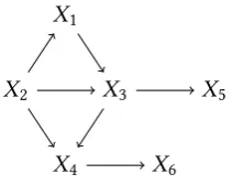
Figure 1.3.An acyclic digraph_Ddepicting conditional independence assumptions on the ran-dom variablesX = (X1, . . . ,X6) which can be equivalently represented by theX-compatible

tree constructed in Example 1.10.

‘x_Ai−1happened before’, whereAi−1=Si_j−₌1₁Ajis the union of all indices in the monomial occur-ring beforeAi andi ≥2. This conditional interpretation is then the same along every root-to-leaf path because the order in whichι_T embeds these states is the same for every atom. Thus,

the primitive probabilitiesθ(xAi)=θ(e(xAi))from (1.16) and (1.17) arepotentialsorkernelsas

in Lauritzen (1996). In particular, they have a conditional or marginal meaning that depends on the graph_T and its sum-to-1 conditions in the parameter spaceΘ_T. As a consequence, the

vec-tors of floret labels of anX-compatible tree are of the typeθv = θ(xAi)|xAi\Ai−1 ∈˜Ai\Ai−1

forv _∈ V. They are thus rows of conditional probability tables of the underlying random

variables.

Consider an illustration below.

Example 1.10(Constructing anX-compatible tree). LetX = (X₁,X₂, . . . ,X₆)be a vector of

random variables with joint probability mass function of the monomial form

pθ(x)=θ(x{1,2,3})θ(x{2,3,4})θ(x{3,5})θ(x{4,6}) (1.19)

for allx _∈ ˜_1×. . ._ט₆as in (1.18). Here,pθ is given in terms of a clique-based

factorisa-tion according to the decomposable acyclic digraph_D in Fig. 1.3. Every indeterminate in the monomial in (1.19) is hence a potential as in Remark 1.9.

We can now draw anX-compatible tree using the embedding

ι_T(x)= e(x_{1,2,3}),e(x{2,3,4}),e(x{3,5}),e(x{4,6}) (1.20)

for allx _∈˜as follows. The root-vertex will correspond to the joint random variableX_{1,2,3} =

(X1,X2,X3)and every emanating edgee(x_{1,2,3}) will correspond to one element in the state space of these three variables, (x1,x2,x3) _∈ ˜1× ˜2× ˜3. These edges are then labelled

by their respective marginal probabilityθ(x_{1,2,3}) = p123(x1,x2,x3). Every child of the root

by the edgee(x_{1,2,3}) corresponds to the random variableX{2,3,4} | X{1,2,3} = x{1,2,3}. Each of these vertices in turn has edgese(x_{2,3,4}) corresponding to states in the space associated to these variables,x_{2,3,4} ∈ ˜2ט3ט4. These edges are now labelled by the conditional

probabilitiesθ(x_{2,3,4})=p4(x4|x2,x3). Continuing in this way, we then attach children to these

vertices which correspond to random variablesX_{3,5}|X{1,2,3} =x{1,2,3},X{2,3,4} =x{2,3,4}and whose edges are labelled byθ(x_{3,5})=p5(x5|x3). To these we finally attach children and leaves

corresponding toX_{4,6} |X{1,2,3} = x{1,2,3},X{2,3,4} = x{2,3,4},X{3,5} = x{3,5} and whose edges are labelled by the conditional probabilitiesθ(x_{4,6})=p6(x6|x4).

The labelled event tree constructed here is now anX-compatible probability tree inducing a

probability mass functionπθ,T◦ιT =pθ which lies in the Bayesian network model{pθ |θ ∈Θ}

of distributions (1.19) which factor according to_D, whereΘis again a product of probability

simplices—one for each row in the conditional probability tables of the components ofX.

Interestingly, we could also have embedded these labels in a different order of vertices and edges: in fact, in any order compatible with_D. Each of the resultingX-compatible trees is then

an alternative representation of the same Bayesian network model and the same tree model: see Example 3.29. Corollary 3.28 on page 93 will state this result in much more generality.

In the development in this section, a certain collection of random variables can be used to construct a labelled event tree which is a probability tree. We will hugely generalise this point in Chapters 2 and 3 where we state conditions under which a collection of monomials can be associated to a tree model.

We will now direct our focus on probability trees which, via an additional graphical property, can capture conditional independence assumptions on distributions which factorise according to their graph. We will then be able to provide expressive illustrations to the concepts intro-duced above, in particular in Example 1.12.

1.2.3. Staged trees

Probability trees are most interesting when two or more florets share the same labels, and distributionsπθ,T factorise according to a ‘coloured’ graphT which captures these equalities. We will analyse this type of model in the remainder of this text.

We first present a definition adapted from Smith and Anderson (2008) and tailored to the development below.

{θ(e) _|e _∈E(v)_{} ∩ {}θ(e0)_|e0_∈E(w)_}=∅for anyv,w _∈ V. We say that two vertices which

have equal floret labels are in the samestage and we denote by∼ the induced equivalence relation on the vertex set.

If no two related vertices lie on the same path,Λ(v)_∩Λ(w)=∅for anyv _∼w, we will call

the staged tree(_T,θ_T)square-free.

For instance, the coin-toss model from the introduction (on page 3) is represented by a staged tree whose two inner vertices are in the same stage. This tree is not square-free.

An interpretation of stage structure is always based on the graph. In particular, given two vertices are in the same stage and a unit arrives at one of them, the transition probabilities to all children of that vertex will not depend on which of the two vertices the unit is actually in, and will thus not depend on the way that unit took to arrive in that situation. The edge (or transition) probabilities in these stages are in this sense independent of their history or location in the tree. See Thwaites and Smith (2015b) for a formal presentation of this type of conditional independence. Note that we will always colour all vertices in the same stage accordingly, as done in Barclay et al. (2013). In doing so, all assumptions on the distributions which factorise according to a staged tree can be coded in a purely graphical way.

When having a preassigned collectionX of random variables as in Section 1.2.2 above,

set-ting vectors of floret labels equal to each other in anX-compatible tree can be interpreted as

specifying a set ofcontext-specificconditional independences of the typeXi ⊥⊥ Xj |Xk = xk for somei,j,k _{∈ {}1, . . . ,m_}. For instance, it is easy to see in Example 1.10 that many of the

constructed vertices will be in the same stage. Indeed, often context-specific constraints hold only on subsets of the state spaces of a collection of random variables. These then provide structure which is additional to the one that can be represented in an acyclic digraph, and this structure is not of graphical nature. Models with these types of constraints are now widely used in BN modelling, especially when the domain of application is large (Boutilier et al., 1996; Smith, 2010).

Just like for Bayesian networks, stage constraints in staged tree models are by construction qualitative assumptions: whatever values two vectors of floret labels take, if their correspond-ing vertices are in the same stage then these labels will be identified. In the symbolic frame-work of later chapters, where we do not assign values to these indeterminates, we will thus often interpret the stage structure of a labelled event tree as a set of linear binomial constraints

θ(e)₋θ(e0) =0 on the edge labels, fore_∈E(v),e0_∈E(v0)andv_∼v0.