Original citation:
Bhattacharya, Sayan, Henzinger, Monika and Nanongkai, Danupon (2017) Fully dynamic
approximate maximum matching and minimum vertex cover in O(log3 n) worst case update
time. In: Twenty-Eighth Annual ACM-SIAM Symposium on Discrete Algorithms, Barcelona,
Spain, 16-19 Jan 2017. Published in: Proceedings of the Twenty-Eighth Annual ACM-SIAM
Symposium on Discrete Algorithms pp. 470-489.
Permanent WRAP URL:
http://wrap.warwick.ac.uk/97558
Copyright and reuse:
The Warwick Research Archive Portal (WRAP) makes this work by researchers of the
University of Warwick available open access under the following conditions. Copyright ©
and all moral rights to the version of the paper presented here belong to the individual
author(s) and/or other copyright owners. To the extent reasonable and practicable the
material made available in WRAP has been checked for eligibility before being made
available.
Copies of full items can be used for personal research or study, educational, or not-for-profit
purposes without prior permission or charge. Provided that the authors, title and full
bibliographic details are credited, a hyperlink and/or URL is given for the original metadata
page and the content is not changed in any way.
Publisher’s statement:
Copyright © 2017 by the Society for Industrial and Applied Mathematics
A note on versions:
The version presented here may differ from the published version or, version of record, if
you wish to cite this item you are advised to consult the publisher’s version. Please see the
‘permanent WRAP URL’ above for details on accessing the published version and note that
access may require a subscription.
Fully Dynamic Approximate Maximum Matching and
Minimum Vertex Cover in
O
(log
3
n
)
Worst Case Update
Time
Sayan Bhattacharya
∗Monika Henzinger
†Danupon Nanongkai
‡Abstract
We consider the problem of maintaining an approximately maximum (fractional) matching and an approximately min-imum vertex cover in a dynamic graph. Starting with the seminal paper by Onak and Rubinfeld [STOC 2010], this problem has received significant attention in recent years. There remains, however, a polynomial gap between the best known worst case update time and the best known amortised update time for this problem, even after allowing for ran-domisation. Specifically, Bernstein and Stein [ICALP 2015, SODA 2016] have the best known worst case update time. They present a deterministic data structure with approxima-tion ratio (3/2 +) and worst case update timeO(m1/4/2), where m is the number of edges in the graph. In recent past, Gupta and Peng [FOCS 2013] gave a deterministic data structure with approximation ratio (1+) and worst case up-date timeO(√m/2). No known randomised data structure
beats the worst case update times of these two results. In contrast, the paper by Onak and Rubinfeld [STOC 2010] gave a randomised data structure with approximation ratio
O(1) and amortised update timeO(log2n), where n is the
number of nodes in the graph. This was later improved by Baswana, Gupta and Sen [FOCS 2011] and Solomon [FOCS 2016], leading to a randomised date structure with approxi-mation ratio 2 and amortised update timeO(1).
We bridge the polynomial gap between the worst case and amortised update times for this problem, without using any randomisation. We present a deterministic data structure with approximation ratio (2 +) and worst case update timeO(log3n), for all sufficiently small constants.
1 Introduction
A matching in a graph is a set of edges that do not share any common endpoint. In the dynamic match-ing problem, we want to maintain an (approximately) maximum-cardinality matching when the input graph
∗Institute of Mathematical Sciences, Chennai, India. Email: [email protected].
†University of Vienna, Faculty of Computer Science. Email:
[email protected]. The research leading to these results has received funding from the European Research Council under the European Union’s Seventh Framework Programme (FP/2007-2013) / ERC Grant Agreement no. 340506.
‡KTH Royal Institute of Technology, Sweden. Email:
[email protected]. Supported by Swedish Research Coun-cil grant 2015-04659 “Algorithms and Complexity for Dynamic Graph Problems”.
is undergoing edge insertions and deletions. The time taken to handle an edge insertion or deletion in the in-put graph is called theupdate timeof the concerned dy-namic algorithm. We want a dydy-namic algorithm whose update time is as small as possible.
We denote the number of nodes and edges in the input graph by n and m respectively. The value of
n remains fixed over time, since the set of nodes in the graph remains the same. However, the value of m
changes as edges get inserted or deleted in the graph. Similar to static problems where we want the running time of an algorithm to be polynomial in the input size, in the dynamic setting we desire the update time to be polylog(n), for an input (edge insertion or deletion) to a dynamic problem can be specified usingO(logn) bits. The dynamic matching problem has been exten-sively studied in the past few years. We now know that within polylog(n) update time we can maintain a 2-approximate matching using a randomized algorithm [15, 1, 13] and a (2 +)-approximate matching using a deterministic algorithm [5, 4, 3]. The downside of these algorithms, however, is that their update times are amortised. Thus, the algorithms take polylog(n) update time on average, but from time to time they may take as large as O(n) time to respond to a single update. It is much more desirable to be able to guaran-tee a small update time after every update. This type of update time is calledworst-case update time.
Unfortunately, known worst-case update time bounds for this problem arepolynomial inn: the known algorithms take O(n1.495) worst-case update time to maintain the value of the maximum matching exactly [14],O(√m/2) time to maintain a (1 +)-approximate maximum matching [8, 12], O(m1/3/2) time to main-tain a (4 +)-approximate maximum matching [4], and
O(m1/4/2) time to maintain a (3/2 +)-approximate maximum matching in bipartite graphs [2]. There is no algorithm with polylog(n) worst-case update time even with a polylog(n) approximation ratio.
We note that the lack of a data structure with good worst-case update time is not at all specific to the
lem of dynamic matching. Other fundamental dynamic graph problems, such as spanning tree, minimum span-ning tree and shortest paths also suffer the same is-sue [7, 9, 10, 6]. One exception is the celebrated ran-domized algorithm with polylog(n) update time for dy-namic connectivity [11].
Our result. We present a deterministic algorithm that maintains a fractional matching1 and a vertex cover2 whose sizes are within a (2 +) factor of each other, for all sufficiently small constants . Since the size of a maximum fractional matching is at most 3/2 times the size of a maximum matching, we can also maintain a (3 +)-approximation to the size of the maximum matching inO(log3n) worst-case update time.
2 A high level overview of our algorithm
In this section, we present the main ideas behind our algorithm. The formal description of the algorithm and the analysis appears in subsequent sections.
Hierarchical Partition. Our algorithm builds on the ideas from a dynamic data structure of Bhattacharya, Henzinger and Italiano [4] called (α, β)-decomposition. This data structure maintains a (2 +)-approximate maximum fractional matching inO(logn/2) amortised update time. It defines the fractional edge weights using levels of nodes and edges. In particular, fix two constants α, β ≥ 1, and recall that the input graph
G = (V, E) has |V| = n nodes. Partition the node set V into L+ 1 levels {0, . . . , L}, where L = logβn. Let`(y)∈ {0, . . . , L} denote the level of a node y∈V. The level of an edge (x, y) is given by Eq. (2.1), and we assign a fractional weightw(x, y) as per Eq. (2.2).
`(x, y) = max(`(x), `(y)) (2.1)
w(x, y) = β−`(x,y)
(2.2)
Thus, the weight of an edge decreases exponentially with its level. The weight of a node y ∈ V is defined as
Wy = P(x,y)∈Ew(x, y). This equals the sum of the weights of the edges incident on it. The goal is to maintain a partition satisfying the following property.
Property 2.1. Every node y with `(y)>0 has weight
1/(αβ) ≤ Wy < 1. Furthermore, every node y with
`(y) = 0 has weight0≤Wy <1.
To provide some intuition, we show how to con-struct a hierarchical partition satisfying Property 2.1
1In a fractional matching each edge is assigned a nonzero weight, ensuring that for every node the sum of the weights of the edges incident to it is at most 1. The size of a fractional matching is the sum of the weights of all the edges in the graph. 2A vertex cover is a set of nodes such that every edge in the graph has at least one endpoint in that set.
in the static setting, when there is no edge inser-tions/deletions. For notational convenience, we de-fine V∗
L = V. Initially, we put all the nodes in level
L, and as per equations 2.1, 2.2 we assign a weight
w(x, y) = β−L = 1/n to every edge (x, y)
∈ E. Since every node has degree at mostn−1, we get 0≤Wy<1 for ally∈VL∗. We now execute aForloop as follows.
Fori=Lto 1:
We partition the node-set Vi∗ into two subsets: Vi =
{y ∈ V : 1/β ≤ Wy < 1} and Vi∗−1 = {y ∈ V : 0 ≤
Wy<1/β}. Next, we move down the nodes inVi∗−1 to level i−1. The level and weight of every edge incident on a node inV \V∗
i−1=Vi∪. . .∪VL remain unchanged during this step, as per equations 2.1 and 2.2. Hence, just after the nodes inV∗
i−1are moved down to leveli−1, we get 1/β ≤ Wy < 1 for all nodes y at level i. The weights of the remaining edges (whose both endpoints lie inV∗
i−1) increase by a factor ofβ. Hence, the weights of the nodes inV∗
i−1also increase by at most a factor of
β. Before the nodes inV∗
i−1 were moved down to level
i−1, we had 0≤Wy<1/βfor ally∈Vi∗−1. Thus, just after the nodes in Vi∗−1 are moved down to level i−1, we get 0≤Wy<1 for ally∈Vi∗−1.
When the above For loop terminates, we have 1/β ≤
Wy < 1 for all nodes y ∈ V at levels `(y) > 0, and 0 ≤ Wy < 1 for all nodes y ∈ V at level `(y) = 0. Specifically, Property 2.1 is satisfied withα= 1.
Theorem 2.1. ([4]) Under Property 2.1, the
edge-weights{w(e)}form a2αβ-approximate maximum frac-tional matching in G.
In [4], Bhattacharya et al. showed that we can dynamically maintain such a partition with α = β = (1 +) inO(logn/2) amortised update time. The main idea is as follows. Assume that we have a partition that satisfies Property 2.1. Now an edge (u, v) is inserted or deleted. This causesWuandWvto increase or decrease. Hence, it might happen that some node x ∈ {u, v}
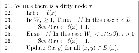
violates Property 2.1 after the insertion/deletion of the edge (u, v), i.e. either (1)Wx ≥1 or (2)Wx <1/(αβ) and`(x)>0. We call such a nodexdirty, and deal with this event by changing the level ofxin a straightforward way as per Figure 1: If Wx is too large (resp. too small), then we increase (resp. decrease) `(x) by one. This causes the weights of some edges incident on xto decrease (resp. increase), which in turn decreases (resp. increases) the value ofWx. For each leveli∈[0, L], we define the set of edges Ei(x) as follows.
Ei(x) ={(x, y)∈E|`(x, y) =i}.
(2.3)
An important observation is that as a nodexmoves up (resp. down) from level i to level i+ 1 (resp. i−1),
the edges whose weights get changed all belong to the set Ei(x). Since the relevant data structures can be maintained efficiently, this implies that the runtime of one iteration of theWhileloop in Figure 1 is dominated
by the cost of Line 7, which takesO(|Ei(x)|) time. In [4], the authors showed that this cost can be amortised over previous edge insertions/deletions.
Note that one iteration of theWhileloop can make
some neighbours of x dirty, and xitself might remain dirty at the end of the iteration. These dirty nodes are dealt with in subsequent iterations in a similar way (until there is no dirty node left).
01. Whilethere is a dirty nodex
02. Leti=`(x)
03. IfWx≥1,Then // In this case i < L
04. Set`(x)←`(x) + 1.
05. Else // In this caseWx<1/(αβ),i >0 06. Set`(x)←`(x)−1.
[image:4.612.63.300.233.324.2]07. Update`(x, y) for all (x, y)∈Ei(x).
Figure 1: Fixing the dirty nodes.
Example: Inserting edges to a star. The following example shows the basic idea behind the amortisation argument. Consider a star centred at nodevconsisting ofβi−1edges, for some largei. To satisfy Property 2.1, we can set `(v) = i, while all other nodes have level 0. Thus, we get Wv = 1/β since every edge has weight 1/βi. Now keep inserting edges to the star (the graph remains a star throughout). Property 2.1 remains satisfied until the (βi
−βi−1)-th edge is inserted – at this point the star consists ofβi edges,W
v = 1, and the node v becomes dirty. We fix the node by increasing
`(v) toi+ 1 as in Algorithm 1, thus reducing the edge-weights to 1/βi+1 and the value of W
v to 1/β. To do this we have to pay the cost of O(|Ei(v)|) = O(βi) in terms of update time. We can amortise this cost over the (βi −βi−1) newly inserted edges. This gives an amortised update time of O(1) for constant β.
Note that in the above example the algorithm does not perform well in the worst case: after the (βi
−βi−1
)-th insertion it has to “probe” all edges inEi(v). So the worst case update time becomes O(βi), which can be polynomial in nwhen iis large. But in this particular instance the problem can be fixed easily: Whenever
v becomes dirty due to the insertion of an edge with weight 1/βi, we reduce the weight of the newly inserted edge and some other edge in the star from 1/βi to 1/βi+1. Thus, the net increase in the weight of v becomes equal to 1/βi−2(1/βi−1/βi+1) = 2/βi+1− 1/βi ≤ 0 (the last inequality holds as long as β ≥2). In other words, when the node v becomes dirty, by
reducing the weights of two edges to 1/βi+1 we can ensure that Wv again becomes smaller than one. Once every edge has weight 1/βi+1, we set `(v) =i+ 1.
Shadow-level (`y(x, y)). To make the above idea concrete, we introduce the notion of ashadow-level. For every node y ∈ V and every incident edge (x, y) ∈ E, we define the shadow-level of y with respect to (x, y), denoted by `y(x, y) ∈ {0, . . . , L}, to be an integer in
{0, . . . , L}such that the following property holds.
Property 2.2. For every node y and edge (x, y),
`(y)−1≤`y(x, y)≤`(y) + 1.
We modify the definition of the level of an edge (x, y)∈E (in Eq. (2.1)) to
`(x, y) = max(`x(x, y), `y(x, y)). (2.4)
This affects the value of w(x, y) and the set Ei(y) as they depend on the levels of edges (see Eq. (2.2) and (2.3)). The idea of the shadow-level is that if
`y(x, y) > `(y) (respectively `y(x, y) < `(y)), then from the perspective of the edge (x, y) we have already increased (resp. decreased) `(y); thus, the level and weight of (x, y) has changed accordingly. In this case, we say thatyup-marks(respectivelydown-marks) the edge (x, y). We will use this operation whenWy is too large (resp. too small). Intuitively, y should not up-mark and down-mark edges at the same time. In particular, let Mdown(y) = {(x, y) ∈E : `y(x, y) = `(y)−1} and
Mup(y) ={(x, y)∈E:`y(x, y) =`(y) + 1}respectively denote the set of all edges down-marked and up-marked byy. Then, we will maintain the following property.
Property 2.3. EitherMup(y) =∅ orMdown(y) =∅.
To see the usefulness of this new definition, consider the following algorithm for dealing with the case where the graph is always a star centred atv: If there are only edge insertions, thenvup-marks the newly inserted edge and another edge inE`(v)(v) whenever it becomes dirty (i.e. Wv≥1). It is easy to see that this will be enough to keepWv <1 as long asβ≥2. OnceE`(v)(v) =∅, we increase `(v) by one. Similarly, if there are only edge deletions, then v can down-mark an edge in E`(v)(v) whenever it becomes dirty (i.e. Wv<1/(αβ)).
The algorithm follows the same strategy when there are both edge insertions and deletions, albeit with one caveat: To ensure that Property 2.3 holds, it cannot up-mark an edge ifMdown(v)6=∅, and cannot down-mark an edge ifMup(v)6=∅. Suppose thatMdown(v)6=∅and we want to reduce the weight of v. In this event, the nodevpicks an edge (u, v) inMdown(v) and sets`v(u, v) back from `(v)−1 to`(v), which reduces the value of
w(u, v). This causes the edge (u, v) to be removed from
··
···
·
··
···
·
··
···
···
·
v
u1
uk
x11
x1j
xk1
xkj
k= i 1/↵
[image:5.612.111.243.85.166.2]j= i 2
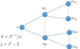
Figure 2: Example. Suppose that i is very large, e.g.
i= (logn)/2, andβ is a large constant.
Mdown(v) and be added to E`(v)(v). We say that the node v un-marks the edge (u, v). Next, suppose that
Mup(v)6=∅and we want to increase the weight ofv. In this event, the nodev un-marks an edge inMup(v).
Failures. So far we have described an idea that leads to small worst-case update time when the input instance is a star graph. To make this idea work on a general input instance, we have to deal with several issues that make the algorithm more complicated. The chief one among them is the observation that the algorithm may fail in adjusting edge weights. Consider, for example, a tree rooted at a node v having k=βi−1/αchildren, sayu1, . . . uk. Further, eachui hasj=βi−2 children. See Fig. 2. Suppose that we satisfy Property 2.1 by setting`(xp,q)←0 for every leaf-nodexp,q withp∈[k] and q ∈[j], `(up)← ifor every internal node up with
p ∈[k], and`(v)← i for the root nodev. No edge is down-marked or up-marked by any node. This implies that Wv = 1/(αβ),Wup = 1−1/β
i for all p
∈[k], and
Wxp,q = 1/β
i for allp
∈[k] andq∈[j].
Now, suppose that the edge (v, u1) gets deleted. This makes v dirty, for Wv becomes smaller than 1/(αβ). The algorithm responds by down-marking an edge in Ei(v), say (v, u2). Unfortunately, this down-marking does not change the weight w(u, v2) since
`v2(u, v2) = i. I We say that this down-marking fails.
When a down-marking fails, the node v remains dirty and Property 2.1 remains unsatisfied. In fact, in this example, the node vwill remain dirty even if we down-mark all the edges inEi(v). To satisfy Property 2.1, we have no other option but to set`(v)←0. However, we cannot do so unless we probe all the edges inEi(v), for we have to ensure that all the down-markings on these edges fail. This takes too much time.
To deal with this issue, we keep down-marking the edges in Ei(v) as long as we fail, until the point when we experience polylog(n) failures. We might still end up having Wv < 1/(αβ). Nevertheless, we will guarantee a constant approximation ratio by arguing that we continue to have Wv = Ω(1/(αβ)). Intuitively, every
time Wv decreases by 1/βi because of these failures, we down-mark many edges in the set Ei(v). Since
|Ei(v)| ≤ βi−1/α, we are able to down-mark all the edges inEi(v) before the value ofWvbecomes too small. At that point, we are ready to decrease the level of v.
Specifically, suppose that the edges inci-dent to v keep getting deleted. While handling
t = βi−1/(αlog2
n) such deletions, we perform
t ·polylog(n) ≥ βi−1/α failed down-markings. This is enough to down-mark every edge in Ei(v). At this point we move v down to level (i−1), and we still have Wv ≥ 1/(αβ)−t/βi = (1−1/log2n)/(αβ). By repeating this argument, we conclude that even if there are more deletions, we still have Wv= Ω(1/(αβ)) until the point in time whenv moves down to level 0 (where
v can not be dirty for its weight being small).
The algorithm in a nutshell. Our algorithm obeys the following principles. When a nodey becomes dirty, it either (1) up-marks or down-marks an edge (x, y), or (2) un-marks an edge (x, y) if up-marking or down-marking would violate Property 2.3. Such an action may fail, meaning that w(x, y) might not change, for reasons exemplified in Fig. 2. In this event,y continues probing its other incident edges, and stops when it experiences either its first success or its polylog(n)th failure. We show: (a) the failures do not cause the weight Wy to become too small or too large, (b) fixing one dirty node leads to at most one new dirty node, and (c) the level of the dirty node under consideration drops after constantly many fixes. Item (a) guarantees a constant approximation factor. Items (b), (c) guarantee a polylog(n) update time, for there areO(logn) levels.
3 Preliminaries
Henceforth, we focus on formally describing our dy-namic algorithm and analysing its worst-case update time. For the rest of the paper, we fix two constants
β, K and define L and f(β) as in equation 3.5. Note that K < Lwhennis sufficiently large.
(3.5) β ≥5, K= 20, f(β) = 1−3/β, L=dlogβne. We will maintain a hierarchical partition of the node-set inG= (V, E), and a fractional matching where the weights assigned to the edges depend on the levels of their endpoints. For technical reasons, however, there will be two key differences between the hierarchical partition actually used by our dynamic algorithm and the one that was defined in Section 2.
1. We will collapse all the nodes in levels{0, . . . , K}into a single level K. Accordingly, the level of a node will lie in the range [K, L] in this new hierarchical partition. The weights of the nodesyin levels`(y)> Kwill satisfy the constraint: f(β)≤Wy <1. On the other hand, the
weights of the nodesy at the lowest level`(y) =Kwill satisfy the constraint: 0 ≤Wy < 1. Comparing these constraints with Property 2.1, it follows that the term 1/(αβ) is replaced byf(β) in the new partition. 2. We will allow the weight of an edge (u, v) to be off by a factor ofβ from its ideal valueβ−max(`(u),`(v)). The structure maintained by our algorithm will be called anice-partition. This is formally defined below.
Definition 3.1. In a nice-partition, the node-setV is
partitioned into (L−K+ 1) subsets VK, . . . , VL. For
i ∈ [K, L], if a node v belongs to Vi, then we say that the node v is at level `(v) = i. Each edge (u, v) ∈ E
gets a weight w(u, v). Let Wv = P(u,v)∈Ew(u, v) be the total weight received by a node v from its incident edges. The following properties hold.
1. For every edge (u, v) ∈ E, we have
β−max(`(u),`(v))−1≤w(u, v)≤β−max(`(u),`(v))+1.
2. If a nodev has `(v)> K, thenf(β)≤Wv<1.
3. If a nodev has `(v) =K, thenWv <1.
Lemma 3.1. Suppose that we can maintain a
nice-partition in O(T(n)) worst-case update time. Then we can also maintain a2/f(β)-approximate maximum frac-tional matching and a 2/f(β)-approximate minimum vertex cover in O(T(n))worst case update time.
Proof. Let Er =
{(u, v) ∈ E : `(u) = `(v) = K} be
the subset of edges with both endpoints at levelK. We will maintain aresidualweightwr(e)
≥0 for every edge
e∈Er. For notational consistency, we definewr(e) = 0 for every edgee∈E\Er. LetWr
v =P(u,v)∈Erwr(u, v) denote the residual weight received by a nodevfrom all its incident edges. Two conditions are satisfied: (a) For each nodev∈V, we have 0≤Wv+Wvr≤1. (b) For every edge (u, v) ∈ Er, we have either W
v +
Wr
v ≥1−1/β orWu+Wur≥1−1/β.
Let degr(v) denote the degree of a node v∈ V among the edges in Er. By condition (1) of Definition 3.1, every edge (x, y) ∈ Er has weight w(x, y)
≥ β−K−1.
Hence, for every node v ∈ V, we get: 1 > Wv ≥
P
(u,v)∈Erw(u, v)≥degr(v)·β−K−1. This implies that degr(v)< βK+1 for every node v
∈V. Sinceβ, K are constants, we get: degr(v) =O(1) for every nodev∈V. Maintaining the residual weights {wr(e)
}, e∈Er.
For every node v ∈ V, let b(v) = 1−Wv denote the capacityof the node. Let br(v) be equal to the value of
b(v) rounded down to the nearest multiple of 1/β. We say that br(v) is the residual capacity of node v. We create anauxiliary graphG∗= (V∗, E∗), where we have
βcopiesof each nodev∈V. For every edge (u, v)∈Er,
there are β2 edges inG∗: one for each pair of copies of
uand v. For each node v∈V, if br(v) =t/β for some integert∈[0, β], thentcopies ofvareturned oninG∗,
and the remaining (β−t) copies ofvareturned offinG∗.
We maintain a maximal matching M∗ in the subgraph
of G∗ induced by the copies of nodes that are turned on. Since degr(v) =O(1) for every nodev∈V, we can maintain the matchingM∗inO(1) update time using a trivial algorithm. From the matching M∗, we get back the residual weights{wr(e)} as follows. For every edge (u, v)∈Er, if there aretedges inM∗between different copies ofuandv, then we setwr(u, v)
←t/β. It is easy to check that this satisfies both conditions (a) and (b). Approximation guarantee.
Condition (a) implies that the edge-weights {w(e) +
wr(e)
} form a valid fractional matching in G. Define the subset of nodes V∗ ={v ∈V :W
v+Wvr ≥f(β)}. Consider any edge (u, v)∈E. If at least one endpoint
x∈ {u, v} lies at a level`(x)> K, then condition (2) of Definition 3.1 implies that Wx+Wxr ≥Wx ≥f(β), and hence x ∈ V∗. On the other hand, if both the
endpoints {u, v} lie at level K, then by conditions (a) and (b) we have: Wx+Wxr≥1−1/β≥f(β) for some
x∈ {u, v}, and hencex∈V∗. It follows thatV∗ forms a valid vertex cover in G. Applying complementary slackness conditions, we infer that the edge-weights
{w(e) +wr(e)} form a 2/f(β)-approximate maximum fractional matching inG, and thatV∗ forms a 2/f(β
)-approximate minimum vertex cover inG.
Fix any constant 0< <1 and letβ = 3(2 +)/. Then β ≥ 5 and 2/f(β) = 2 + (see equation 3.5). Setting β in this way, we can use Theorem 3.1 and Lemma 3.1 to maintain a (2+)-approximate maximum fractional matching and a (2+)-approximate minimum vertex cover in O(log3n) worst-case update time. We devote the rest of the paper to proving Theorem 3.1.
Theorem 3.1. We can maintain a nice-partition in
G= (V, E)inO(log3n)worst case update time.
3.1 Shadow-levels. As in Section 2, the shadow-levels will uniquely determine the weight w(u, v) as-signed to every edge (u, v)∈E. They will ensure that
w(u, v) differs from the ideal value β−max(`(u),`(v)) by at most a factor ofβ. This implies condition (1) of Def-inition 3.1. Specifically, we require that each edge has two shadow-levels: one for each of its endpoints. Let
`y(x, y)∈ [K, L] be the shadow-level of a node y with respect to the edge (x, y). We require that this shadow-level can differ from the actual shadow-level of the node by at most one. This is formally stated in the invariant below.
Invariant 1. For every node y ∈ V and every edge
(x, y)∈E, we have `(y)−1≤`y(x, y)≤`(y) + 1.
Next, as in Section 2, we define thelevel of an edge to be the maximum value among the shadow-levels of its endpoints. Let `(x, y) ∈ [K, L] be the level of an edge (x, y). Then for every edge (x, y)∈E we have:
(3.6) `(x, y) = max(`x(x, y), `y(x, y)).
As in Section 2, we now require that the weight assigned to an edge (u, v)∈E be given byβ−`(u,v).
(3.7) w(x, y) =β−`(x,y) for every edge (u, v)∈E.
Thus, the weight of an edge decreases exponentially with its level. It is easy to check that if Invariant 1 holds, then assigning the weights to the edges in this manner satisfies condition (1) of Definition 3.1.
Corollary 3.1. Suppose that Invariant 1 holds and
edges are assigned weights as in equations 3.6, 3.7. Then for every edge (x, y)∈E we have:
β−max(`(x),`(y))−1≤w(x, y)≤β−max(`(x),`(y))+1.
Proof. Since each shadow-level differs from the actual level by at most one (see Invariant 1), the maximum value among the shadow-levels also differs from the maximum value among the actual levels by at most one. Specifically, we get: max(`(x), `(y))−1 ≤ `(x, y) = max(`x(x, y), `y(x, y)) ≤ max(`(x), `(y)) + 1. The corollary now follows from the fact that the weight of an edge (x, y)∈E is given byw(x, y) =β−`(x,y).
As in Section 2, we now define the concept of an edge marked by a node. Consider any edge (x, y)∈ E
incident to a nodey∈V. If`y(x, y) =`(y) + 1, then we say that the edge (x, y) has beenup-markedby the node
y. Similarly, if`y(x, y) =`(y)−1, then we say that the edge (x, y) has been down-marked by the nodey. And if`y(x, y) =`(y), then we say that the edge (x, y) is un-marked by the node y. We let Mup(y) and Mdown(y) respectively be the set of all edges (x, y)∈ E incident toy that have been up-marked and down-marked byy. For everyi∈[K, L], we letEi(y) be the set of all edges (x, y)∈E incident toy that are at level`(x, y) =i.
Mup(y) = {(x, y)∈E:`y(x, y) =`(y) + 1} (3.8)
Mdown(y) = {(x, y)∈E:`y(x, y) =`(y)−1}
(3.9)
Ei(y) = {(x, y)∈E:`(x, y) =i}
(3.10)
3.2 Different states of a node. Our goal is to maintain a nice-partition in G. In Section 3.1, we defined the concept of shadow-levels so as to ensure that the edge-weights satisfy condition (1) of Definition 3.1. In this section, we present a framework which will ensure that the node-weights satisfy the remaining conditions
(2), (3) of Definition 3.1. Towards this end, we first need to define the concept of anactivationof a node.
Activations of a node. The deletion of an edge (x, y) inGleads to a decrease in the values ofWxandWy. In contrast, when an edge (x, y) is inserted inG, we assign values to its two shadow-levels `x(x, y) and `y(x, y) in such a way that Invariant 1 holds, and then assign a weight to the edge as per equation 3.7. This leads to an increase in the values ofWx andWy. These two events are called natural activations of the endpoints x, y. In other words, a node isnaturally activated whenever an edge incident to it is either inserted into or deleted from
G. The weight of a node changes whenever it encounters a natural activation. Hence, such an event might lead to a scenario where the node-weight becomes either too large or too small, thereby violating either condition (2) or condition (3) of Definition 3.1. For example, consider a nodeyat a level`(y)> Kwhose current weight is just slightly smaller than one. Thus, we have: 1−δ≤Wy< 1 for some smallδ. Now, suppose thaty gets naturally activated due to the insertion of an edge (x, y). Further, suppose that this leads to the value of Wy becoming larger than one after the natural activation. So the node y violates condition (2) of Definition 3.1. In our algorithm, at this stage the nodey will select some edge (x0, y) ∈E
`(y)(y) and up-mark that edge. Specifically, the node will set `y(x0, y) ← `(y) + 1, insert the edge
(x0, y) into the setsMup(y) andE`(y)+1(y), and remove
the edge from the setE`(y)(y). The new level of the edge will be given by`(x0, y) =`(y) + 1. This will reduce the
node-weightWybyβ−`(y)−β−(`(y)+1), and (hopefully) the new value ofWywill again be smaller than one. The up-marking of the edge (x0, y), however, will change the
weight of the other endpoint x0. We call such an event
an induced activation of x0. Specifically, an induced activation of a node x0 refers to the event when the node-weight Wx0 increases (resp. decreases) because
the other endpoint y of an incident edge (x0, y) has decreased (resp. increased) its shadow-level`y(x0, y).
In general, consider an activation of a node y that increases its weight. Suppose that the node wants to revert this change (weight increase) so as to ensure that conditions (2) and (3) of Definition 3.1 remain satisfied. Then it either up-marks some edges fromE`(y)(y) or un-marks some edges from Mdown(y). This, in turn, might activate some of the neighbours ofy.
Similarly, consider an activation of a node y that decreases its weight. Suppose that the node wants to revert this change (weight decrease) so as to ensure that conditions (2) and (3) of Definition 3.1 remain satisfied. Then it either down-marks some edges fromE`(y)(y) or un-marks some edges from Mup(y). Again, this might in turn activate some of the neighbours ofy.
We require that a node cannot simultaneously have an up-marked and a down-marked edge incident on it. This requirement is formally stated in Invariant 2. Intuitively, a node has up-marked incident edges when it is trying to ensure that its weight does not become too large, and down-marked incident edges when it is trying to ensure that its weight does not become too small. Thus, it makes sense to assume that a node cannot simultaneously be in both these states.
Invariant 2. For every node y ∈V, eitherMup(y) =
∅ orMdown(y) =∅.
Invariant 3 states that if a nodeyhas up-marked or down-marked an incident edge (x, y), then the shadow-level `x(x, y) of the other endpoint x is no more than the level ofy. Intuitively, the nodeyup-marks or down-marks an incident edge only if it wants to change its weightWywithout changing its own level`(y). Suppose that the invariant is false, i.e., the nodeyhas up-marked or down-marked an edge (x, y) with `x(x, y) > `(y). Then we have `y(x, y) ≤ `(y) + 1 ≤ `x(x, y), where the first inequality follows from Invariant 1. But, this implies that y can never change the weight w(x, y) by up-marking or down-marking (x, y), for the value of
w(x, y) is determined by the shadow-level of the other endpoint x. Thus, the node y does not gain anything by up-marking or down-marking the edge (x, y). This is why we guarantee the following invariant.
Invariant 3. For every edge (x, y)∈E, if `y(x, y)6=
`(y), then we must have`x(x, y)≤`(y).
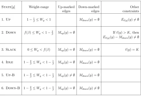
Six different states. For technical reasons, we will require that a node is always in one of six possible states. See Table 1. It is easy to check that this is sufficient to ensure conditions (2), (3) of Definition 3.1. See Lemma 3.2. One way to classify these states is as follows. Definition 3.1 requires that the weight of a node
y lies in the range 0≤Wy<1. We partition this range into four intervals: I1, I2, I3 andI4. These intervals are non-empty as long asβ is a sufficiently large constant.
I1= [0, f(β)), I2= [f(β),1−2/β)
I3= [1−2/β,1−1/β) and I4= [1−1/β,1).
A node y is in Up state when Wy ∈ I4, Down state
when Wy ∈ I2, and Slack state when Wy ∈ I1. As per Table 1, the node y has to satisfy some additional constraints whenState[y]∈ {Up,Down,Slack}.
Fi-nally, ifWy∈I3, thenyis in one of three possible states
–Idle,Up-B,Down-B– depending on whether or not
it has up-marked or down-marked any incident edge. By Invariant 2, a node cannot simultaneously up-mark
some incident edges and down-mark some other incident edges. Hence, three cases can occur when Wy∈I3. (a)
Mup(y) =Mdown(y) =∅. In this caseyis inIdlestate.
(b) Mdown(y) =∅and Mup(y)6=∅. In this casey is in
Up-Bstate. (c)Mup(y) =∅andMdown(y)6=∅. In this
casey is inDown-B state.
The six states are precisely defined in Table 1.
Lemma 3.2. If a node y ∈ V is in one of the states
described in Table 1, then its weight Wy satisfies condi-tions (2) and (3) of Definition 3.1.
Proof. In every state, we have 0≤Wy<1 (see Table 1). We consider two mutually exclusive and exhaustive cases. (a) f(β) ≤ Wy < 1. (b) 0 ≤ W < f(β). In case (a), clearly the node-weightWy satisfies conditions (2), (3) of Definition 3.1. In case (b), the node must be in Slack state (see Table 1), and so we must have
`(y) = K. Thus, the node satisfies conditions (2), (3) of Definition 3.1 even in case (b).
Note that each of the intervals I1, I2, I3 and I4 defined above is of length at least 1/β(see equation 3.5). On the other hand, for every edge (u, v) ∈E we have
w(u, v) ≤ 1/βK, for K is the minimum possible level in a nice-partition. Accordingly, a natural or induced activation of a node can change its weight by at most 1/βK. Note that 1/βK is much smaller than 1/β. This apparently simple observation has an important implication, namely, that a node must be activated at leastβK−1times for its weight to cross the feasible range of any interval in {I1, I2, I3, I4}. As a corollary, if a node y has, say, Wy ∈I3 just before getting activated, then the activation can only moveWyto aneighbouring interval –I2orI4. But it is not possible to haveWy∈I3 just before the activation, and Wy ∈ I1 just after the activation. Throughout the rest of the paper, we will be using this observation each time we consider the effect of an activation on a node. Next, we will briefly explain the motivation behind considering all these different states.
1. State[y] =Up. See row (1) in Table 1.
A nodeyis inUpstate when 1−1/β≤Wy <1. In this state the node’s weight is close to one. Hence, whenever its weight increases further due to an activation the node tries to up-mark some incident edges from E`(y)(y), in the hope that this would reduce the node’s weight and ensure that Wy never exceeds one. The node y can up-mark an edge only if the set E`(y)(y) is nonempty. Hence, we require that E`(y)(y)6=∅. Further, to ensure that a up-marking does not violate Invariant 2, we require thatMdown(y) =∅.
2. State[y] =Down. See row (2) in Table 1.
A nodeyis inDownstate whenf(β)≤Wy <1−2/β. In this state the node’s weight is close to the threshold
State
[
y
]
Weight-range
Up-marked
Down-marked
Other
edges
edges
constraints
1.
Up
1
−
β1≤
W
y<
1
M
down(
y
) =
∅
E
`(y)(
y
)
6
=
∅
2.
Down
f
(
β
)
≤
W
y<
1
−
β2M
up(
y
) =
∅
If
`
(
y
)
> K
, then
E
`(y)(
y
)
−
M
down(
y
)
6
=
∅
3.
Slack
0
≤
W
y< f
(
β
)
M
up(
y
) =
∅
M
down(
y
) =
∅
`
(
y
) =
K
4.
Idle
1
−
β2≤
W
y<
1
−
β1M
up(
y
) =
∅
M
down(
y
) =
∅
5.
Up-B
1
−
β2≤
Wy
<
1
−
β1Mup
(
y
)
6
=
∅
Mdown
(
y
) =
∅
[image:9.612.69.546.219.543.2]6.
Down-B
1
−
β2≤
W
y<
1
−
β1M
up(
y
) =
∅
M
down(
y
)
6
=
∅
Table 1: Constraints satisfied by a node in different states.
f(β). There are two cases to consider here, depending on the current level of the node.
2-a. `(y) > K. In this case, whenever the value of
Wy decreases further due to an activation, the node tries to down-mark some incident edges fromE`(y)(y)\
Mdown(y), in the hope that this would increase the node’s weight and ensure that Wy does not drop below the thresholdf(β). The nodeycan down-mark an edge only if the setE`(y)(y)\Mdown(y) is nonempty. Hence, we require that E`(y)(y)\Mdown(y)6=∅. Furthermore, in order to ensure that a down-marking does not violate Invariant 2, we require that Mup(y) =∅.
2-b. `(y) = K. In this case, the node y cannot down-mark any incident edge (x, y), for we must always have `y(x, y) ∈ [K, L]. Thus, we get Mdown(y) = ∅ in addition to the constraints specified in row (2) of Table 1. If an activation makes Wy smaller than f(β), then we simply setState[y]←Slack.
We highlight one apparent discrepancy between the statesUpandDown. If a nodeyis inDownstate with
`(y)> K, then it tries to down-mark some edges from
E`(y)(y)\Mdown(y) after an activation that reduces its weight. However, if the same node is in Upstate, then
it tries to up-mark some edges from E`(y)(y) after an activation that increases its weight. This discrepancy is due to the fact that E`(y)(y)∩Mup(y) =∅, as every edge (x, y)∈Mup(y) has `(x, y)≥`y(x, y) =`(y) + 1. In other words, an edge up-marked by y can never belong to the setE`(y)(y), and henceE`(y)(y)\Mup(y) =
E`(y)(y). In contrast, an edge (x, y)∈Mdown(y) belongs to the set E`(y)(x, y) if`x(x, y) =`(y).
3. State[y] =Slack. See row (3) in Table 1.
A node y is in Slack state when 0 ≤ Wy < f(β). In order to ensure condition (2) of Definition 3.1, we require that the node be at level K. Since K is the minimum possible level, there is no need for the node to prepare for moving down to a lower level in future. Hence, we require that Mdown(y) = ∅. Further, the node’s weight is currently so small that it will take quite some time before the node has to prepare for moving up to a higher level. Hence, we require thatMup(y) =∅.
4. State[y] =Idle. See row (4) in Table 1.
A nodeyis inIdlestate when 1−2/β≤Wy<1−1/β and Mup(y) =Mdown(y) =∅. In this state the node’s weight is neither too large nor too small, and the node does not have any up-marked or down-marked incident edges. Intuitively, the node need not worry even if its weight changes due to an activation in this state. In other words, when a node gets activated inIdle state,
it does not up-mark, down-mark or un-mark any of its incident edges. After a sufficiently large number of activations when the node’s weight drops below (resp.
rises above) the threshold 1−2/β (resp. 1−1/β), it switches to the state Down(resp. Up).
5. State[y] =Up-B. See row (5) in Table 1. The term
“Up-B” stands for “Up-Backtrack”.
A nodeyis inUp-Bstate when 1−2/β≤Wy<1−1/β,
Mup(y)6=∅andMdown(y) =∅. Intuitively, this state of the node captures the following scenario. Some time back the node y was in Up state with 1 − 1/β ≤
Wy < 1, Mup(y) =6 ∅ and Mdown(y) = ∅. From that point onward, the node encountered a large number of activations that kept on reducing its weight. Eventually, the value of Wy became smaller than 1−1/β and the node entered the stateUp-B. If the node keeps getting
activated in this manner, then in near future Wy will become smaller than 1−2/β and the nodey will have to enter the state Down. At that time we must have
Mup(y) =∅. In other words, the node y has to ensure that Mup(y) = ∅ before its weight drops below the threshold 1−2/β. Thus, whenever State[y] = Up-B
and the node-weightWydecreases due to an activation, the nodey un-marks some edges fromMup(y).
6. State[y] =Down-B. See row (6) in Table 1. The
term “Down-B” stands for “Down-Backtrack”.
A node y is inDown-B state when 1−2/β ≤ Wy < 1−1/β, Mdown(y) 6= ∅ and Mup(y) = ∅. Intuitively, this state of the node captures the following scenario. Some time back the node y was in Down state with
f(β)≤Wy <1−2/β, Mdown(y)6=∅ andMup(y) =∅. From that point onward, the node encountered a large number of activations that kept on increasing its weight. Eventually, the value ofWybecame greater than 1−2/β and the node entered the state Down-B. If the node
keeps getting activated in this manner, then in near future Wy will become greater than 1−1/βand it will have to enter the stateUp. At that time we must have
Mdown(y) =∅. In other words, the nodeyhas to ensure that Mdown(y) = ∅ before its weight increases beyond the threshold 1−1/β. Thus, whenever State[y] =
Down-B and Wy increases due to an activation, the
node yun-marks some edges fromMdown(y).
3.3 Dirty nodes. Our algorithm maintains a bit
D[y]∈ {0,1}associated with each node y∈V. We say that the nodeyisdirtyifD[y] = 1 andcleanotherwise. Intuitively, the node y is dirty when it is unsatisfied about its current condition and it wants to up-mark, down-mark or un-mark some of its incident edges. Once a dirty node is done with up-marking, down-marking or un-marking the relevant edges, it becomes clean again. In our algorithm, a node becomes dirty only after it encounters a natural or induced activation. The converse of this statement, however, is not true. There may be times when a node remains clean even after
getting activated, and this will be crucial in bounding the worst-case update time of our algorithm. Whether or not a node will become dirty due to an activation depends on: (1) the state of the node, (2) the type of the activation under consideration (whether it increases or decreases the node-weight), and (3) the node’s current level. We have three rules that determine when a node becomes dirty.
Rule 3.1. A node y with State[y] ∈ {Up,Down-B}
becomes dirty after an activation that increases its weight. In contrast, such a node does notbecome dirty after an activation that decreases its weight.
Justification for Rule 3.1.
Case 1. State[y] = Up. Here, we have 1−1/β ≤
Wy < 1 and Mdown(y) = ∅. If an activation increases the value of Wy, then y needs to up-mark some edges fromE`(y)(y), in the hope thatWyremains smaller than 1 (see the discussion in Section 3.2). Hence, the node becomes dirty. In contrast, if an activation reduces the value of Wy, then y need not up-mark, down-mark or un-mark any of its incident edges. Due to this inaction, if it so happens that 1−2/β≤Wy <1−1/βafter the activation, then the node simply switches to stateUp-B
or Idledepending on whether or notMup(y)6=∅.
Case 2. State[y] = Down-B. Here, we have 1 −
2/β ≤ Wy < 1−1/β, Mdown(y) 6= ∅ and Mup(y) =
∅. Such a node must un-mark all its incident edges before its weight rises past the threshold 1−1/β (see the discussion in Section 3.2). Hence, whenever its weight increases due to an activation and State[y] =
Down-B, the nodeybecomes dirty and un-marks some
edges from Mdown(y). In contrast, if an activation reduces its weight, then the node y need not up-mark, down-mark or un-mark any of its incident edges. Due to this inaction, if it so happens thatf(β)≤Wy<1−2/β after the activation, then we set State[y] ← Down.
At this point, if we have E`(y)(y)\Mdown(y) = ∅ and
`(y)> K, then the nodey moves to a lower level while being inDownstate (see Case 2-b in Section 4.1).
Rule 3.2. Consider a node y such that either (1)
State[y] = Down and `(y) > K, or (2) State[y] =
Up-B. This node becomes dirty after an activation that
decreases its weight. In contrast, the node does not be-come dirty after an activation that increases its weight.
Justification for Rule 3.2.
Case 1. State[y] = Down and `(y) > K. Thus, we
have f(β) ≤ Wy < 1−2/β and Mup(y) = ∅. If an activation decreases its weight, then y needs to down-mark some edges fromE`(y)(y)\Mdown(y), in the hope that Wy does not become smaller than f(β) (see the
discussion in Section 3.2). Hence, the node y becomes dirty. In contrast, if an activation increases its weight, thenyneed not up-mark, down-mark or un-mark any of its incident edges. Due to this inaction, if it so happens that 1 −2/β ≤ Wy < 1−1/β after the activation, then the node simply switches to stateDown-BorIdle
depending on whether or notMdown(y)6=∅.
Case 2. State[y] = Up-B. Thus, we have 1−2/β ≤
Wy < 1 −1/β, Mup(y) 6= ∅ and Mdown(y) = ∅. Such a node must un-mark all its incident edges before its weight drops below the threshold 1−2/β (see the discussion in Section 3.2). Hence, whenever its weight decreases due to an activation and State[y] = Up-B,
the node y becomes dirty and un-marks some edges from Mup(y). In contrast, if an activation increases its weight, then y need not up-mark, down-mark or un-mark any of its incident edges. Due to this inaction, if it so happens that 1−1/β≤Wy<1 after the activation, then we set State[y]←Up. At this point, if we have
E`(y)(y) = ∅, then the node y moves to a higher level while being inUp state (see Case 2-a in Section 4.1).
Rule 3.3. A node y with either (1) State[y] ∈
{Slack,Idle} or (2) {State[y] = Down and `(y) =
K} never becomes dirty after an activation.
Justification for Rule 3.3.
Case 1. State[y] =Slack. Here, we have 0≤Wy <
f(β), Mup(y) = Mdown(y) = ∅ and `(y) = K. When such a node gets activated, it need not up-mark or down-mark any of its incident edges. Due to this inaction, if it so happens that f(β) ≤ Wy < 1 −2/β after the activation, then we setState[y]←Down.
Case 2. State[y] = Idle. Here, we have 1−2/β ≤
Wy < 1−1/β and Mup(y) = Mdown(y) = ∅. When such a node gets activated, it need not up-mark or down-mark any of its incident edges. Due to this inaction, if it so happens that 1−1/β≤Wy<1 after the activation, then we set State[y]←Up. At this point, if we have
E`(y)(y) = ∅, then the node y moves to a higher level while being in Up state (see Case 2-a in Section 4.1).
In contrast, if it so happens thatf(β)≤Wy <1−2/β after the activation, then we set State[y] ← Down.
At this point, if we have E`(y)(y)\Mdown(y) =∅ and
`(y)> K, then the nodey moves to a lower level while being inDownstate (see Case 2-b in Section 4.1).
Case 3. State[y] = Down and `(y) = K. Thus, we
have f(β) ≤ Wy < 1−2/β and Mup(y) = ∅. Since
`(y) =Kand`y(x, y)∈[K, L] for every edge (x, y)∈E, we also have Mdown(y) = ∅. When such a node gets activated, it need not up-mark or down-mark any of its incident edges. Due to this inaction, if we have 0≤
Wy< f(β) after the activation, then we setState[y]←
Slack. In contrast, if 1−2/β ≤Wy <1−1/β after the activation, then we setState[y]←Idle.
Corollary 3.2. If an activation of a nodey makes it
dirty, then the state of the node remains the same just before and just after the activation (see Section 6.1).
Proof. While justifying Rules 3.1 – 3.3, whenever we changed the state of the node y due to an activation, we ensured that the node did not become dirty.
3.4 Data structures. In our dynamic algorithm, ev-ery nodey∈V maintains the following data structures. 1. Its weight Wy, level `(y), and state State[y] ∈
{Up, Down, Slack, Idle, Up-B, Down-B}.
2. The setsMup(y), Mdown(y) as balanced search trees. 3. A bitD[y]∈ {0,1} to indicate if the nodey isdirty. 4. For every level i∈ {0, . . . , L}, the set of edgesEi(y) as a balanced search tree.
Furthermore, every edge (x, y)∈Emaintains the values of its weightw(x, y) and level`(x, y).
Remark about maintaining the shadow-levels.
Note that we do not explicitly maintain the shadow-level `x(x, y) of a nodey ∈V with respect to an edge (x, y)∈E. This is due to the following reason.
For the sake of contradiction, suppose that our algorithm in fact maintains the values of the shadow-levels `y(x, y). Consider a scenario where the node y
has State[y] = Up, `(y) = i, and the value of Wy
is very close to one. Next, suppose that an activation increases the value ofWy, and the node up-marks one or more edges from the set Ei(y) to ensure that the value of Wy remains smaller than one. Since `(x, y) = i+ 1 for every edge (x, y)∈Mup(y), all the newly up-marked edges get deleted from the set Ei(y) and added to the set Ei+1(y). At this point, we might end up in a situation where Ei(y) = ∅, which violates a constraint of row (1) in Table 1. Our algorithm deals with this issue by moving the node y up to level (i+ 1), i.e., by setting `(y)← (i+ 1). Since Ei(y) = ∅, this does not affect the weight of any edge. However, for every edge (x, y)∈E with`(x, y)> i+ 1, the shadow-level`y(x, y) changes from i to (i+ 1). Since each edge (x, y) ∈ E
with `(x, y) > i+ 1 has weight at most β−(i+2), and sinceWy <1, there can be βi+2−1 many such edges. Accordingly, the nodey might be forced to change the values of the shadow-levels `y(x, y) for O(βi+2) many edges (x, y). The worst-case update time then becomes
O(βi+2), which is polynomial in nfor large values ofi. We avoid this problem by giving up on explicitly maintaining the values of the shadow-levels `y(x, y). Still we can determine the value of `x(x, y) inO(logn)
time from the data structures that are in fact main-tained by us. Specifically, we know that if (x, y) ∈
Mup(y), then `y(x, y) = `(y) + 1. Else if (x, y) ∈
Mdown(y), then `y(x, y) = `(y)−1. Finally, else if (u, y)∈/Mup(y)∪Mdown(y), then`y(x, y) =`(y).
For ease of exposition, we nevertheless use the no-tation `y(x, y) while describing our algorithm in subse-quent sections. Whenever we do this, the reader should keep it in mind that we are implicitly computing`y(x, y) as per the above procedure.
4 Some basic subroutines
4.1 The subroutine UPDATE-STATUS(y).
This subroutine is called each time a node y experi-ences a natural or an induced activation. This tries to ensure, by changing the state and level ofyif necessary, that y satisfies the constraints specified in Table 1. If the subroutine fails to ensure this condition, then our algorithm HALTS. During the analysis of our algorithm, we will prove that it never HALTS due to a call to UPDATE-STATUS(y). This implies that every node satisfies the constraints in Table 1, and hence Lemma 3.2 guarantees that conditions (2) and (3) of Definition 3.1 continue to remain satisfied all the time. We say that a node is fit in a state X ∈
{Up,Down,Slack,Idle,Up-B,Down-B} if it
satis-fies all the constraints for state X as specified in Ta-ble 1, and unfit otherwise. If D[y] = 1, then our al-gorithm HALTS if y is unfit in its current state. In contrast, if D[y] = 0, then our algorithm HALTS if y
is unfit in every state, albeit with one caveat: If the node is unfit in either stateUpor stateDown, then we
first try to make it fit in that state by changing its level
`(y). Hence, there is a sharp distinction between the treatments received by the clean nodes on the one hand and the dirty nodes on the other. Specifically, the state of a node y can change during to a call to UPDATE-STATUS(y) only if y is clean at the beginning of the call. This distinction comes from Corollary 3.2, which requires that a node does not change its state if it be-comes dirty. We now describe the subroutine in details.
Case 1. D[y] = 1. The node yis dirty.
If y is fit in its current state, then we terminate the subroutine. Otherwise our algorithm HALTS.
Case 2. D[y] = 0. The node yis clean.
If we can find some state X ∈
{Up,Down,Slack,Idle,Up-B,Down-B} in which
y is fit, then we set State[y] ←X and terminate the
subroutine. Else if the node y is unfit in every state, then we consider the sub-cases 2-a, 2-b and 2-c.
Case 2-a. The node is unfit in state Up only due to
the last constraint in row (1) of Table 1. Thus, we have
1−1/β≤Wy<1,Mdown(y) =∅andE`(y)(y) =∅. Let
i←`(y) be the current level ofy. We find the minimum level j > iwhere Ej(y)6=∅. Such a levelj must exist since Wy > 0. We move the node y up to level j by setting `(y) ← j. This does not change the weight of any edge. Furthermore, when the node was in level i, we had `y(x, y) ≤`(y) + 1≤ i+ 1≤j for every edge (x, y)∈E incident ony (see Invariant 1). Hence, after the node moves up to levelj, we have`y(x, y) =j=`(y) for every edge (x, y) ∈ E. In other words, the node y
is not supposed to have any up-marked edges incident on it just after moving to level j. Accordingly, we set
Mup(y)← ∅. Then we terminate the subroutine.
Case 2-b. The node is unfit in state Down only due
to the last constraint in row (2) of Table 1. Thus, we have f(β) ≤ Wy < 1−2/β, Mup(y) = ∅, E`(y)(y)\
Mdown(y) = ∅ and `(y) > K. Let i ← `(y) be the current level ofy. We first move the node down to level
i−1 by setting`(y)←i−1. We claim that this does not change the level (and weight) of any edge. To see why the claim is true, consider any edge (x, y)∈E incident on y. Since Mup(y) = ∅, we must have `y(x, y) ≤ i
just before the node moves down to level (i−1). If
`x(x, y) ≥ i, then the value of `(x, y) is determined by the other endpoint xand the level of such an edge does not change as y moves down to level (i−1). In contrast, if`x(x, y)< i, then we have (x, y)∈Mdown(y): for otherwise the edge (x, y) will belong to the set
Ei(y)\Mdown(y) which we have assumed to be empty. The level of such an edge remains equal to (i−1) as the node y moves down from level i to level (i−1). This concludes the proof of the claim that the edge-weights do not change as y moves down from level i to level (i−1). Next, consider any edge (x, y) that was down-marked when the node y was at level i. At that time, we had `y(x, y) = i−1. Hence, after the node moves down to leveli−1, we get`y(x, y) =i−1 =`(y). Thus, the node cannot have any down-marked edge incident on it just after moving down to leveli−1. Accordingly, we set Mdown(y) ← ∅. At this point, if we find that
Ei−1(y) = ∅, then we move the node further down to
the lowest levelK, by setting`(y)←K. This does not change the level and weight of any edge in the graph. Finally, we terminate the subroutine.
Case 2-c. In every scenario other than 2-a and 2-b described above, our algorithm HALTS.
A note on the space complexity. In cases 2-a and 2-b of the above procedure, there is a step where we set Mup(y) ← ∅ and Mdown(y) ← ∅ respectively. It is essential to execute this step in O(poly logn) time: otherwise we cannot claim that the update time of our algorithm is O(poly logn) in the worst-case. Unfortunately for us, there can be Ω(β`(y)) many edges
in the set Mup(y) or Mdown(y). Hence, it will take Ω(β`(y)) time to empty that set if we have to delete all those edges from the corresponding balanced search tree. Note that β`(y)= Ω(n) for large`(y).
To address this concern, we maintain two pointers
root[Mup(y)] and root[Mdown(y)] for each node y∈V. They respectively point to the root of the balanced search tree for Mup(y) and Mdown(y). When we want to set Mup(y) ← ∅ or Mdown(y) ← ∅, we respectively setroot[Mup(y)]←NULL orroot[Mdown(y)]←NULL. This takes only constant time. The downside of this ap-proach is that the algorithm now uses up a lot of junk space in memory: This space is occupied by the bal-anced search trees that wereemptied in the past. As a result, the space complexity of the algorithm becomes
O(tpoly logn) for handling a sequence oft edge inser-tions/deletions starting from an empty graph. This is due to the fact that our algorithm will be shown to have a worst-case update time of O(poly logn). Hence, we can upper bound the total time taken to handle these edge insertions/deletions byO(tpoly logn), and this, in turn, gives a trivial upper bound on the amount ofjunk spaceused up in the memory.
A standard way to bring down the space complexity is to run aclean-upalgorithm in the background. Each time an edge is inserted into or deleted from the graph, we visit O(poly logn) memory cells that are currently junk andfree them up. Thus, the worst case update time of the clean-up algorithm is alsoO(poly logn), and this increases the overall update time of our scheme by only a O(poly logn) factor. The size of all setsMup(.) and
Mdown(.) that exist at a given point in time is O(m). Hence, this clean-up algorithm is at most O(m) space “behind”, i.e., the additional space requirement for junk space is O(m). For ease of exposition, from this point onward we will simply assume that we can empty a balanced search tree inO(1) time.
Lemma 4.1. The subroutine UPDATE-STATUS(y)
takes O(logn)time.
Proof. Case 1 can clearly be implemented in O(1) time. In case 2-a, we have to find the minimum level j > i where Ej(y) 6= ∅. This operation takes time proportional to the number of levels, which is
L−K+ 1 =O(logn). Everything else takesO(1) time. Finally, case 2-b and case 2-c also take O(1) time.
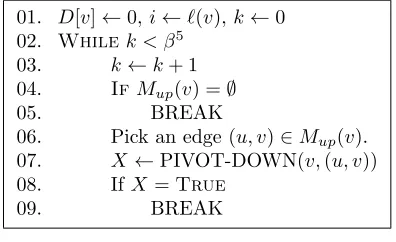
4.2 The subroutine PIVOT-UP(v,(u, v)). This is described in Figure 3. This subroutine is called when the nodev is dirty and it wants to increase its shadow-level `v(u, v) with respect to the edge (u, v). There are two situations under which such an event can take place: (1) State[v] =Up and v wants to up-mark the
edge (u, v), and (2) State[v] =Down-B and v wants
to un-mark the edge (u, v). The subroutine PIVOT-UP(v,(u, v)) updates the relevant data structures, de-cides whether the node ushould become dirty because of this event, and returnsTrueif the event changes the
weight of the edge (u, v) andFalseotherwise. Thus, if
the subroutine returns True, then this amounts to an
induced activation of the nodeu.
The subroutine MOVE-UP(v,(u, v)). Step (01) in Figure 3 calls another subroutine MOVE-UP(v,(u, v)). This subroutine updates the relevant data structures as the value of `v(u, v) increases by one, and returns
Trueif the weightw(u, v) gets changed andFalse
oth-erwise. To see an example where MOVE-UP(v,(u, v)) returns False, consider a situation where State[v] =
Down-B, `(v) = i, `v(u, v) = i−1, and `u(u, v) =
`(u) = i. In this instance, even after the node v in-creases the value of `v(u, v) by un-marking the edge (u, v), the weightw(u, v) does not change.
The subroutine MOVE-UP(v,(u, v)) ensures that Invariant 3 remains satisfied. Specifically, after the value of`v(u, v) increases we might have`v(u, v)> `(u), and then we must ensure that the edge (u, v)∈/ Mup(u)∪
Mdown(u): otherwise Invariant 3 will be violated (set
y = u and x = v in Invariant 3). If we end up in this situation, then the subroutine MOVE-UP(v,(u, v)) removes the edge fromMup(u)∪Mdown(u).
01. Y ←MOVE-UP(v,(u, v))
02. IfY =Trueandeither State[u] =Up-Bor
(State[u] =Downand`(u)> K)
03. D[u]←1 04. UPDATE-STATUS(u) 05. RETURNY.
Figure 3: PIVOT-UP(v,(u, v)).
Deciding if the node u becomes dirty. We now continue with the description of the subroutine PIVOT-UP(v,(u, v)). After step (01) in Figure 3, it remains to decide whether the node u should become dirty. This decision is made following the three rules specified in Section 3.3. Note that if we increase the value of
`v(u, v), then it can never lead to an increase in the weightWu. Thus, ifY =True, then it means that the
weight Wu dropped during the call to the subroutine MOVE-UP(v,(u, v)). On the other hand, ifY =False,
then it means that the weightWudid not change during the call to the subroutine MOVE-UP(v,(u, v)). In this event, the node unever becomes dirty.
As per Rules 3.1 – 3.3, if the weight Wu gets reduced, then u becomes dirty iff either State[u] =
Up-B or (State[u] =Down, `(u)> K). Thus, the
subroutine setsD[u]←1 iff two conditions are satisfied: (1) Y = True, and (2) either State[u] = Up-B or
(State[u] =Down, `(u)> K).
Finally, just before terminating the subroutine PIVOT-UP(v,(u, v)) in Figure 3, we call the subrou-tine UPDATE-STATUS(u). The reason for this call is explained in the beginning of Section 4.1.
Lemma 4.2. The subroutine PIVOT-UP(v,(u, v))
takes O(logn) time. It returns True if the weight
w(u, v) gets changed, and False otherwise. The node
ubecomes dirty only if the subroutine returns True.
Proof. A call to the subroutine UPDATE-STATUS(y) takes O(logn) time, as per Lemma 4.1. The rest of the proof follows from the description of the subroutine.
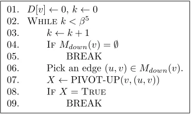
4.3 The subroutine PIVOT-DOWN(v,(u, v)).
This is described in Figure 4. This subroutine is called when the node v is dirty and it wants to decrease its shadow-level `v(u, v) with respect to the edge (u, v). There are two situations under which such an event can take place: (1) State[v] =Down and v wants to
down-mark the edge (u, v), and (2) State[v] =Up-B
and v wants to un-mark the edge (u, v). The subrou-tine PIVOT-DOWN(v,(u, v)) updates the relevant data structures, decides whether the node u should become dirty, and returnsTrueif the weight of the edge (u, v)
gets changed andFalseotherwise. Thus, if the
subrou-tine returnsTrue, then this amounts to an induced
ac-tivation of the nodeu. This subroutine, however, is not a mirror-image of the subroutine PIVOT-UP(v,(u, v)). The difference between them is explained below.
In the subroutine PIVOT-DOWN(v,(u, v)), sup-pose that the nodevhas decreased the value of`v(u, v), and this has increased the weight Wu. Furthermore, the nodeuis currently in a state where Rules 3.1 – 3.3 dictate that it should become dirty when its weight in-creases. If this is the case, then the node uattempts to undo its weight-change by increasing the value of
`u(u, v). To take a concrete example, suppose that just before the subroutine PIVOT-DOWN(v,(u, v)) is called, we have State[v] =Up-B, `(v) =i, `v(u, v) =
i+ 1, State[u] =Up, `(u) =i and `u(u, v) =i. The
node v now decreases the value of `v(u, v) by one, and un-marks the edge (u, v). Thus, the weight w(u, v) changes from β−(i+1) to β−i. This also increases the weight Wu by an amount β−i−β−(i+1). The node u will now undo this change by up-marking the edge (u, v), which will increase `u(u, v) by one. This will bring the weightWuback to its initial value. In contrast, the sub-routine PIVOT-UP(v,(u, v)) does not allow the nodeu
to perform such “undo” operations. This “undo” opera-tion performed byuin PIVOT-DOWN(v,(u, v)) will be