Tractable consideration set structures for assortment optimization and network revenue management

warwick.ac.uk/lib-publications

Original citation:

Strauss, Arne and Talluri, Kalyan. (2017) Tractable consideration set structures for

assortment optimization and network revenue management. Production and Operations

Management.

Permanent WRAP URL:

http://wrap.warwick.ac.uk/84313

Copyright and reuse:

The Warwick Research Archive Portal (WRAP) makes this work by researchers of the

University of Warwick available open access under the following conditions. Copyright ©

and all moral rights to the version of the paper presented here belong to the individual

author(s) and/or other copyright owners. To the extent reasonable and practicable the

material made available in WRAP has been checked for eligibility before being made

available.

Copies of full items can be used for personal research or study, educational, or not-for profit

purposes without prior permission or charge. Provided that the authors, title and full

bibliographic details are credited, a hyperlink and/or URL is given for the original metadata

page and the content is not changed in any way.

Publisher’s statement:

"This is the peer reviewed version of the following article: Strauss, Arne and Talluri, Kalyan.

(2017) Tractable consideration set structures for assortment optimization and network

revenue management. Production and Operations Management., which has been published

in final form at

http://doi.org/10.1111/poms.12685

This article may be used for

non-commercial purposes in accordance with

Wiley Terms and Conditions for Self-Archiving

."

A note on versions:

The version presented here may differ from the published version or, version of record, if

you wish to cite this item you are advised to consult the publisher’s version. Please see the

‘permanent WRAP URL’ above for details on accessing the published version and note that

access may require a subscription.

Tractable consideration set structures for assortment optimization

and network revenue management

Arne K. Strauss

_{, Kalyan Talluri}

7 October 2016

Abstract

Discrete-choice models are widely used to model consumer purchase behavior in assortment optimization

and revenue management. In many applications, each customer segment is associated with a

consider-ation set that represents the set of products that customers in this segment consider for purchase. The

firm has to make a decision on what assortment to offer at each point in time without the ability to

iden-tify the customer’s segment. A linear program called the Choice-based Deterministic Linear Program

(CDLP_{) has been proposed to determine these offer sets. Unfortunately, its size grows exponentially}

in the number of products and it is NP-hard to solve when the consideration sets of the segments

over-lap. The Segment-based Deterministic Concave Program with some additional consistency equalities

(SDCP_{+) is an approximation of}CDLP _{that provides an upper bound on}CDLP_{’s optimal objective}

value. SDCP+ can be solved in a fraction of the time required to solve CDLP and often achieves

the same optimal objective value. This raises the question under what conditions can one guarantee

equivalence ofCDLP andSDCP+. In this paper, we obtain a structural result to this end, namely that

if the segment consideration sets overlap with a certain tree structure or if they are fully nested,CDLP

can be equivalently replaced with SDCP_{+. We give a number of examples from the literature where}

this tree structure arises naturally in modeling customer behavior.

Keywords: discrete choice models, assortment optimization, network revenue management, consideration sets

1

Introduction

This paper is concerned with three closely related problems: The Assortment Optimization problem is to

determine an assortment of products to maximize the expected revenue from a heterogenous population of

customers. This population is modeled as being made up of multiple latent customer segments. Revenue

management (RM) is dynamic assortment optimization for products that share a common resource. In

Network Revenue Management (NRM), products may use inventory from multiple resources (for example, a

hotel stay for three nights uses three days of inventory; airline itineraries involving multiple flights use seats

on the connecting flight legs). Network interactions arise as the decision to offer a product depends on the

future revenues attainable from the sale of the other products that share resources on the network.

Underlying all three problems is a model of how consumers choose a product to purchase. Talluri and

van Ryzin [18] introduced RM based on a discrete-choice model of customer purchases. Discrete-choice

models represent purchase probability as a function of available products and customer characteristics. Such

modeling was later applied to NRM by Gallego, Iyengar, Phillips, and Dubey [7] and Liu and van Ryzin [12]

who formulated a Choice-based Deterministic Linear Program (CDLP), the main object1 _{of study in this}

paper. The linear programCDLP has an exponential number of variables and is difficult to solve except for

a few restricted choice models.

In our model, the customer population consists of multiple segments. Each segment is associated with a

subset of products called the consideration set, along with segment-specific parameters of the choice model.

Assuming that all products are available, the consideration set represents the set of products that customers

in that segment would consider for purchase. Consideration sets play a crucial role in the solvability of the

assortment optimization problem: If the segments’ consideration sets overlap, the assortment optimization

problem is NP-hard when there are just two segments, even for simple choice models such as the

Multinomial-Logit (MNL) (Bront, M´endez-D´ıaz, and Vulcano [5]).

Motivated by this intractability of CDLP, Talluri [19] develops a weaker formulation called

Segment-based Deterministic Concave Program (SDCP), weaker in the sense that its optimal objective value gives an

upper bound on the optimal objective value ofCDLP. The idea is to solve a collection of small subproblems,

each corresponding to a segment, with some constraints that loosely link them together. SDCP is generally

poor in approximatingCDLP when segment consideration sets overlap, i.e. its optimal objective function

value is significantly higher than that of CDLP, and it also performs poorly in revenue simulations. To

improve this situation, Meissner, Strauss, and Talluri [14] propose an extension of the SDCP formulation

calledSDCP+ (defined in§2.4) that obtains a significantly tighter relaxation ofCDLP for the case of over-lapping consideration sets. In their numerical experiments,SDCP+ achieves theCDLP optimal objective

function value in many instances despite being faster to solve by an order of magnitude.

The main contribution of this paper is that we identify two consideration set structures for whichCDLP

is equivalent toSDCP+, i.e. a solution to CDLP can be obtained by instead solving the simpler problem

SDCP+ with significantly fewer decision variables in a fraction of computation time. We give a number of

applications from the literature where such consideration set structures naturally occur in the modeling of

customer behavior. Our results depend only on the consideration set structure and not on the structure of

the network of resources and, importantly, apply for any general discrete-choice model.

The remainder of the paper is organized as follows: In §2 we introduce the notation, the demand model,

the basic dynamic program and the two approximations of the dynamic program, namely the CDLP and

theSDCP+. In§3 we present the main structural results. In §4 we illustrate some applications from the literature where the desired structure of the consideration set is naturally present. In§5 we summarize our conclusions.

2

Models

We introduce the notation in§2.1. In§2.2, we state a dynamic programming formulation of the choice-based NRM problem. Its intractability motivates the formulation of approximations: in§2.3 we define the Choice-based Deterministic Linear Program (CDLP), and in §2.4 the Enhanced Segment-Based Deterministic

Concave Program (SDCP+).

2.1

Notation

A product is a specification of a price (usually with restrictions such as advance purchase requirements)

combination of fare class (price and restrictions) and the itinerary (the flight legs of the itinerary); in a hotel

network, a product is a multi-night stay for a particular room type at a certain price point.

We define a discrete-time booking horizon that consists of T intervals, indexed by t. The sale process

begins at time 0 and all resources perish instantaneously at timeT. We make the standard assumption that

the time intervals are small enough so that the probability of more than one customer arriving in a time

period is negligible.

The underlying network has mresources (indexed by i) andnproducts (indexed byj), and we refer to

the set of all resources as I and the set of all products as J. The resources used by j are represented by

a resource-product incidence matrix A, with aij = 1 if product j uses resource i, and aij = 0 otherwise.

Columns ofA are the 0-1 incidence vectorsAj. We denote the vector of capacities at time t as ct, so the

initial set of capacities at time 0 isc0.

We assume that there are L:={1, . . . , L}customer segments, each with distinct purchase behavior. In each period, a customer arrives with probabilityλand belongs to segmentl with probabilitypl. We denote

λl=plλand assume P_l∈Lpl= 1, so λ=P_l∈Lλl. We assume time-homogenous arrivals (homogenous in

rates and segment mix), but the model and all solution methods in this paper can be clearly extended to

the case where rates and mix change by period. Customers in segmentl have aconsideration set Cl ⊆J

of products that they consider to purchase (see Shocker et al. [17] for a survey on the consideration-set

modeling literature).

In each period the firm offers a subset S of its products for sale, called theoffer set. Given an offer set

S, an arriving customer purchases a productj (at the pricerj) in the setS or decides not to purchase any

(no-purchase). The no-purchase option is indexed by 0 and is always present for the customer.

A segment-l customer’s choice probabilities are not affected by the availability of productsj ∈J\Cl. A

segment-lcustomer purchasesj∈S ifj∈S∩Cl with probabilityPjl(S), S⊆J. These functions are either

given by an oracle or by a functional form such as in the MNL model wherePl

j(S) =vlj/(Pk∈Cl∩Svlk) for

a set of “weights”vl∈R|Cl| that capture the attractiveness of the products for each segmentl.

Whenever we specify probabilities for a segment l for a given offer set S, we just write it with respect

to Sl =Cl∩S (note that Pjl(S) = Pjl(Sl)). So when the firm offers setS, it sellsj ∈ S with probability

We define the vector Pl_{(S) = [P}l

1(Sl), . . . , Pnl(Sl)] (recall the no-purchase option is indexed by 0, so

it is not included in this vector). We define the vector P(S) = [P1(S), . . . , Pn(S)]. Notice that P(S) =

P

l∈LplPl(S). We define the vectorsQl(S) =APl(S) andQ(S) =AP(S) to denote the expected resource

consumption for an offer set S by segment l. Likewise, the expected revenue function for segment l is

Rl_{(S) =}P

j∈SlrjP

l

j(Sl) and the expected revenue from a given arrival,R(S) =Pj∈SrjPj(S).

In our notation and demand model we broadly follow Bront et al. [5] and Liu and van Ryzin [12].

2.2

Dynamic Program

We describe the stochastic dynamic program to determine the optimal offer set at each point in time. While

computationally intractable, it gives a conceptual reference point of the value we are trying to approximate

with tractable methods.

Let Vt(ct) denote the maximum expected revenue that can be earned over the remaining time horizon

[t, T], given remaining capacityctin periodt. LetJ(ct) denote the set of products thatcanbe offered given

remaining available capacity, i.e.,J(ct) :={j∈J|Aj ≤ct}. ThenVt(ct) satisfies the Bellman equation

Vt(ct) = max S⊆J(ct)

 

 X

j∈S

λPj(S)

rj+Vt+1(ct−Aj)

+λP0(S) + 1−λ

Vt+1(ct)

 



, ∀t,∀ct, (1)

with the boundary condition VT(cT) = 0 for all cT. Let VDP := V0(c0) denote the optimal value of this

dynamic program from 0 toT, for the given initial capacity vectorc0. Solving the dynamic program (1) is

intractable because the state space explodes even for small problems. Therefore, we are forced to look at

approximations to the dynamic program (1).

2.3

Choice Deterministic Linear Program (

C DLP

₎

The Choice-based Deterministic Linear Program (CDLP) approximation defined in Gallego et al. [7] and

Liu and van Ryzin [12] has 2n _{decision variables w}

decision variables can be interpreted as the amount of time setS is offered:

max X

S⊆J

λR(S)wS

s.t. X

S⊆J

λwSQ(S)≤c0

(CDLP) X

S⊆J

wS =T (2)

0≤wS, ∀S ⊆J.

That is, we maximize the total expected revenue, subject to the constraint that the total expected capacity

consumption on each resourceimust be less than or equal to the initially available capacityc0i. The second

constraint (2) says that we offer product sets overT time units.

Liu and van Ryzin [12] show that the optimal objective value of CDLP is an upper bound on VDP_.

They also show that the problem can be solved efficiently by column generation for the MNL model with

non-overlapping segment consideration sets. Bront et al. [5] and Rusmevichientong, Shmoys, Tong, and

Topaloglu [16] investigate this further and show that column generation is NP-hard if the consideration sets

for the segments overlap for the MNL choice model with two segments.

2.4

Enhanced Segment-Based Deterministic Concave Program (

SDC P

₊

₎

Talluri [19] proposed an upper bound onCDLP called the Segment-based Deterministic Concave Program

(SDCP). SDCP optimizes the offer set for each segment separately. SDCP and CDLP have the same

objective values when the consideration sets for the different segments are disjoint. We do not elaborate on

theSDCP formulation as it is not considered further in this paper, but it corresponds to the formulation

(SDCP+) given below without the constraints (4).

In applications, the segments’ consideration sets can overlap in a variety of ways and, as the choice

probabilities depend on the offer set, they do not have any structure that we can exploit. We call a set

of constraints valid for a linear programming approximation of the dynamic program (1) if adding the

constraints preserves the property that its optimal objective value still forms an upper bound on VDP_.

below—that tighten theSDCP bound. We call the formulationSDCP+ in light of the additional constraints

(4). LetSlmrepresent subsets ofCl∩Cm, i.e., subsets in the intersection of the consideration sets of segments

l andm. SDCP+ is:

max

L

X

l=1 X

Sl⊆Cl

λlRl(Sl)wlSl

s.t.

(SDCP+)

L

X

l=1

yl≤c₀ (3)

X

Sl⊆Cl

λlQl(Sl)wSll≤yl, ∀l∈ L

X

Sl⊆Cl wl

Sl=T, ∀l∈ L

X

{Sl⊆Cl|Sl⊇Slm} wl

Sl−

X

{Sm⊆Cm|Sm⊇Slm} wm

Sm = 0,

∀Slm ⊆Cl∩Cm,∀ {l, m} ⊂ L:Cl∩Cm6=∅ (4)

wl

Sl≥0, ∀Sl⊆Cl,∀l∈ L,

yl≥0, ∀l∈ L.

The vectorylrepresents capacity allocation to segmentlsubject to total available capacityc0. We maximize

total expected revenue from each segment l subject to several constraints. The first represents that the

capacity allocations are limited by the overall available network capacity. The second set enforces that each

segment can only consume at most as many resources as have been allocated to it. The third ensures that

we offer product sets (possibly the empty set) over the full time horizon. The intuition behind the product

cuts (4) is the following: SDCP+ can be seen as a collection of segment-level implementations of CDLP

linked via the constraint (3) and tightened via the product cuts (4). For any setSlm⊂Cl∩Cm, the length

of time that setSlm is offered to segmentl(possibly alongside other products) must be equal to the length

of time that it is being offered to segment m (again possibly alongside other products). The numerical

experiments of Meissner et al. [14] show that generating just a few of these constraints can be sufficient to

3

Analysis of

C DLP

_and

SDC P

₊

We wish to understand when the optimal objective value of SDCP+ is the same as CDLP. To this

end, we first develop a simple example to illustrate that there can be a strict gap between the

opti-mal objective values of CDLP and SDCP+, even if all product cuts are satisfied. The underlying

rea-son for that gap is that there is no solution to CDLP that can be projected onto the segment

con-sideration sets so as to coincide with the segment-level optimal solution. When are these two

formu-lations equivalent then? We explore this issue in the remainder of this section following the example.

A

B

C

1 2

3 4

5

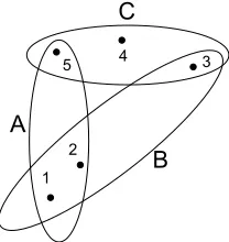
Figure 1: Consideration sets for 3 segments,

5 products

Example 1 Our example has five products and three

seg-ments and their respective consideration sets are shown in

Fig-ure 1. For this example we show that there is a gap between

the optimal objective values ofSDCP+ andCDLP even if we

generate all constraints of type (4). Assume T = 1, capacity

c = 1, revenue rj = 1 for all products j ∈ J ={1,2,3,4,5},

λl = 1/3 for all segments l ∈ {A, B, C}, and the purchase

probabilities defined as follows: PA

j ({1,2}) := 0.5 forj= 1,2,

PA

j ({2,5}) := 0.5 forj = 2,5,P2B({2}) := 1,PjB({1,2,3}) :=

1/3 forj= 1,2,3,PC

4 ({4}) := 1 andPjC({3,5}) := 0.5 forj= 3,5, and 0 for all other sets.

We show that there is a feasible solution to SDCP+ for this example with objective value 1. A feasible

solution toSDCP+ is given byyl= 1/3 for all segmentsl, andw{A1,2}=w{A2,5}= 0.5,wB{2}=wB{1,2,3}= 0.5,

wC

{4} = wC{3,5} = 0.5, and wlSl = 0 otherwise for all l ∈ {A, B, C}, Sl ⊂ Cl. This solution is feasible to SDCP+ since λlP_Sl⊆ClQ

l_(S

l)wlSl = 1/3 = yl for all segments l, and the product cuts (4) for all pairs

of segments{l, m} and sets Slm ⊂Cl∩Cm, Slm 6=∅ are satisfied as reported in Table 1. They also hold

for Slm = ∅ since the solution satisfies P_Sl⊆Clw

l

Sl = 1 for all segments l. The other constraints are

like-wise satisfied as can easily be checked. The objective value is 1 since λlP_Sl⊆ClR

l_(S

l)wlSl = 1/3 for each l∈ {A, B, C}.

Next, we show that there is no corresponding solution to CDLP with the same objective value. Note that

A

B

C

{1,2}=

C

∩C

{3}=

C

∩C

{5}=

C

∩C

Figure 2: Intersection graph for the example in Figure 1.

described above, we can enumerate all 32 subsets S and calculate the corresponding objective coefficient

λR(S). We find that λR(S) ≤ 2/3 for all S ⊂ J, with equality reached for the sets {1,2,3}, {1,2,4},

{2,3,5}, {1,2,3,4} and {1,2,3,5}. It follows that there can be no feasible solution to CDLP that has objective value greater than 2/3 since the objective is a convex combination of these coefficients (note that

T = 1).

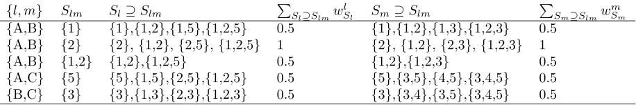
{l, m} Slm Sl⊇Slm P_Sl⊇Slmw

l

Sl Sm⊇Slm

P

Sm⊇Slmw

m Sm

{A,B} {1} {1},{1,2},{1,5},{1,2,5} 0.5 {1},{1,2},{1,3},{1,2,3} 0.5

{A,B} {2} {2},{1,2},{2,5},{1,2,5} 1 {2},{1,2},{2,3},{1,2,3} 1

{A,B} {1,2} {1,2},{1,2,5} 0.5 {1,2},{1,2,3} 0.5

{A,C} {5} {5},{1,5},{2,5},{1,2,5} 0.5 {5},{3,5},{4,5},{3,4,5} 0.5

{B,C} {3} {3},{1,3},{2,3},{1,2,3} 0.5 {3},{3,4},{3,5},{3,4,5} 0.5 Table 1: Evaluation of all product cuts (4) for the example given in Figure 1.

Moving on from the example, we seek to obtain a structural result on when CDLP and SDCP+ are

equivalent. Since the overlap of the consideration sets plays a critical role in Example 1, let us represent the

overlap structure in a graph. Specifically, we define a bipartiteintersection graph as follows: There are two

types of nodes, one type called segment node, the other is called intersection node. Each node of the former

type corresponds to a segment, each of the latter represents a set of the formCk∩Clfor some segment pair

(k, l). If there are two pairs of segments (m, n) and (k, l) with Cm∩Cn =Ck∩Cl, then S =Cm∩Cn is

represented by a single intersection node. Edges from segment node k connect to all the sets of the form

Ck∩Cl6=∅ for anyl6=k. In graph theory, a connected graph without cycles is called a tree, and a disjoint

union of trees is called a forest [4].

The intersection graph of the example of Figure 1 has a cycle, as can be seen from Figure 2. This turns

out to be the critical feature: If the segment consideration sets do not have a cycle and are arranged say

in the form of a tree (or, in general, a forest), then the product cuts are sufficient to ensure equivalence

some intuition for it: The intersection tree tells us which segments are directly or indirectly connected to

each other, in the sense that a solution wl _{for some segment l is dependent on the solution w}k _{for any}

segment nodekthat is reachable from segment nodel. Example 1 illustrates this point: It is not possible to

arrange the segment-level solutions in a way such that they are consistent. By consistent, we mean that there

is a feasible solution to CDLP that can be projected onto the segments to obtain theSDCP+ solution.

For instance, if we would arrange the SDCP+ solution so that the sets SA

1 ={1,2}, S1B ={1,2,3}, and SC

1 ={3,5} are offered in parallel (recall that they are all offered for the same duration), then we cannot

find a single set S ⊂ J whose projection onto the segment consideration sets results in SA

1, S1B and S1C,

respectively. To see this, note that SA

1 requires us not to offer product 5, whereas S1C does require us to

offer product 5. In fact, there is no possibility to arrange the segment-level solutions so that all sets that

would be offered in parallel are consistent, and this shows that the segment-level solutions of Example 1 do

not have a correspondingCDLP solution.

The product cuts ensure that any offer set in the intersection of any two segments’ consideration sets is

being offered to both segments for the same time (possibly alongside offering other products). This is the

case in Example 1: All sets are offered for the same duration. Suppose we have a tree-structured intersection

graph with a segment node l connected to a segment nodek via a single intersection node. For a given

solution wl_{, the product cuts allow us to arrange the segment-level solutions w}k _{in a way such that they}

represent the projections of a feasible global solution onto the respective segments. We can repeat this

argument to construct a globalCDLP solution by moving along the tree. However, if there is a cycle, then

this pairwise approach to construct a global solution does not work any more because there is no guarantee

that the last segment-level solution (wC _{in Example 1) in the sequence along the cycle is consistent with the}

first segment-level solution (wA _{in Example 1).}

Proposition 1. If the intersection graph is a forest, then CDLP and SDCP+ have the same optimal

objective value (henceforth referred to by the shorthand notation CDLP =SDCP+).

Proof

A

B

U

wA_(S 1)

wA(S2) w B_(S

3)

wB(S4)

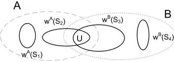
Figure 3: Merging procedure used in the proof of Proposition 1.

example with two segments, A and B, displayed in Figure 3 along with their corresponding consideration

sets. Figure 3 shows a feasible solution toSDCP+. We wish to construct a feasible solution toCDLP from

this solution with the same objective value. For simplicity assume that the only sets with positive weights

that contain U are S2 in the consideration set of A and S3 in the consideration set ofB. Note that the

product cuts imply the restriction wA S2 =w

B

S3 since S2 and S3 are the only offer sets with positive weight

in the segment-level solution for segments A andB respectively that contain the set U in the intersection

of the consideration sets. Moreover, wA S1 +w

A

S2 = T and w

B S3+w

B

S4 = T. This implies that w

A S1 =w

B S4.

So we construct weights for the CDLP formulation as wCDLP

S1∪S4 = w

A S1 = w

B

S4 and w

CDLP

S2∪S3 = w

A S2 = w

A S3.

This CDLP solution satisfies wCDLP

S1∪S4+w

CDLP

S2∪S3 =T, as well as the capacity constraints, and has the same

objective value as theSDCP+ solution.

In the proof of Proposition 1 (see appendix), we essentially repeat this argument for the more complicated

case with Lsegments and arbitrary consideration sets using an induction argument (made possible by the

tree structure).

✷

In addition to the tree-structured intersection graphs, we identify another structure that guarantees

equivalence of CDLP and SDCP+. We show that nested consideration sets also guarantee CDLP =

SDCP+ even though such consideration sets do not have the tree structure.

Proposition 2. For a nested consideration set structureC1⊆C2⊆. . .⊆CL,CDLP =SDCP+.

Proof

See appendix.

✷

step in the proof of Proposition 1 is a merging procedure between a leaf node and the rest of the intersection

graph. What we require is that at every step we should be able to find a leaf node. Once we identify the

leaf node (segment), and remove it, the intersection graph of the remaining segments can be quite different

from the original. Indeed, that is the reason for the tractability of the nested consideration structure in

Proposition 2 even though the original intersection graph is not a tree. Hence, we can write a more general

version of Proposition 1 as follows:

Proposition 3. CDLP is equivalent to SDCP+ when the intersection graph has a sequence of

segment-nodes, such that the first node in the sequence is a leaf node, and after removal of each leaf node and a

re-drawing of the intersection graph with the remaining segments the next segment-node in the sequence is

also a leaf node in the new intersection graph.

4

Applications

In this section we present some applications from the literature where the consideration set structures that

we have described appear naturally in the modeling. These applications are: RM of advance tickets and

ticket options for sport events (§4.1), RM for primary care clinics (§4.2), dynamic pricing of home delivery time slots (§4.3), low cost airlines (§4.4), and retail (§4.5).

4.1

Revenue management of advanced tickets and options for sports tickets

Sport event ticket options have become so popular that there is a software company called TTR that

specializes in selling Internet platforms to teams and events that wish to offer options. Balseiro, Gocmen,

Gallego, and Phillips [2] consider a scenario where advance tickets for the tournament are sold before it

starts—hence the identities of the two teams playing in a tournament final are unknown at this time.

However, fans of a specific team are only interested in attending the event if their team makes it to the final.

To address this uncertainty, the authors propose team-specific call options under which a customer can pay

a small non-refundable amount in advance for the right to attend the event if and only if the specified team

makes it to the final and if he pays an additional amount once the finalists are known. Such options allow

event organizers in principle to oversell capacity many times because only fans with advance tickets or with

1

2

L

...

΂΃ O1

O2 _A OL

...

Figure 4: A star consideration structure (left) and the corresponding intersection graph (right) in sports RM.

support; assuming there areLteams in the tournament in total, we therefore haveLcustomer segments. A

customer from segmentl has the choice between buying an advance ticket Athat would give access to the

final regardless of who will be playing, and an optionOl _{for team l. In other words, a customer in segment}

l has a consideration set{A, Ol_{}. Thus we obtain a star consideration set structure (Figure 4).}

Balseiro et al. [2] use the CDLP to solve the problem, and show for their specific model that an

equiv-alent, more compact formulation exists that actually is special case of SDCP+. The main result of our

paper provides a more general explanation for the equivalence of CDLP and SDCP+, namely that the

consideration set structure is a tree.

4.2

Revenue management for primary care clinics

Gupta and Wang [8] present an application of revenue management under patient choice of primary care

providers and appointment time-slots. Specifically, the problem is to manage physicians’ consultation time

slot availabilities over a finite booking horizon so as to maximize revenues. Each physician has a panel of

patients for whom he is the designated primary-care provider; these patient groups correspond to customer

segments with preferences for particular physicians. Patients of any segment can choose between all available

combinations of all appointment time-slots and all physicians, hence the consideration sets are all identical.

Same-day patients form another segment and are assumed to be willing to accept any available slot with any

physician on the workday. In this application, the product is a combination of physician-time combination.

All patient segments consider all products, and therefore the intersection tree has a star structure as in

the previous example. Gupta and Wang [8] proposed various heuristics to tackle the problem; our main

result tells us that we can use the tractableSDCP+ formulation in lieu ofCDLP as an alternative solution

4.3

Dynamic pricing of home delivery time-slots

Another application related to appointment scheduling is the work of Asdemir, Jacob, and Krishnan [1]

who look at the question of how to dynamically price delivery time-slots for attended home delivery over

a finite booking horizon using dynamic programming. Different prices can be quoted for different delivery

time-slots at any given point in time. There are different customer segments in a given area based on a

choice model that reflects their preferences for specific time-slots as well as price sensitivity. Their model

considers all geographic areas as independent of each other. All segments in a given area are assumed to

consider all available delivery time-slots. If the time slot prices have to be the same across all segments

within a given geographical area (which would be reasonable so as to avoid customer dissatisfaction due to

perceived unfairness of this group-based discrimination), we again have a star-shaped tree as the intersection

graph. Similar to the previous application, the geographic area and time-slot combination is the product.

As solution method, Asdemir et al. [1] propose a dynamic program that has an exponentially growing

state space in the number of delivery time-slots. Alternatively, one could again useSDCP+ (equivalent to

CDLP owing to the tree structure) to obtain an approximate policy that can be calculated even for large

problem instances where dynamic programming becomes intractable.

4.4

Nested consideration set structure (low-cost airline model)

Consider a fully nested consideration set structure where the L consideration sets are nested as C1 ⊆ C2 ⊆. . .⊆CL. This models buy-up/buy-down amongst unrestricted products where complete dilution is

possible. This type of structure is encountered on single-leg flights or in a retail context where customers

remove products from consideration based on certain cutoff values for the products’ attributes or qualities,

and these can be ranked linearly. The latter example was proposed by Feldman and Topaloglu [6] to motivate

work on assortment optimization under MNL with nested consideration sets. Proposition 2 shows that this

is tractable, following the structure defined in Propostion 3.

4.5

Retail

When defining segments and their consideration sets, there is often a certain degree of subjectivity and

5 4 3 2 1 P C B A

{A,B,C,P} {P} {C} {B} {A}

4’ 3’ 2’ 1’ P C B A

{B,C} {A,B} {P} {C} {B} {A}

2’

3’

4’

{B,C} {A,B}

Figure 5: Intersection graph for the retail data set in [9] (left), transformed after merging segment 5 and 3 and after reducing consideration sets to those with purchase probability greater than 10% (middle), and after removing leaf nodes as in Proposition 3 (right).

and Russell [9]. Initially, they discover nine customer segments with intersection graph as illustrated on the

left of Figure 5. There are four loyal segments for the brands A, B, C and P, respectively, and five switching

segments. They found that segment 5 and segment 3 could be merged without major impact on the preference

structure. Furthermore, one could refine the sets of the switching segments by including only the products

with purchase probabilities greater than 10% (the threshold mentioned in Kamakura and Russell [9]). The

resulting simplified consideration sets of the modified segments 1′_{, 2}′_{, 3}′_{, 4}′ _{were{A},{A,B},{A,B,C} and}

{B,C,P}, respectively. The corresponding intersection graph is depicted in the middle of Figure 5 along with the simple tree structure on the right that results from removing leaf nodes as in Proposition 3. This serves as

an example of how a modeler could sensibly change the segmentation so as to obtain a tractable structure;

effectively it comes down to balancing the loss in modeling accuracy with tractability of the subsequent

5

Conclusions

Discrete-choice models are widely used to model consumer purchase behavior in assortment optimization

and revenue management. The firm has to make a decision on what assortment to offer at each point in

time without the ability to identify the customer’s segment. In many applications, each customer segment

is associated with a consideration set that represents the set of products that customers in this segment

consider for purchase. The formulationCDLP has been proposed to determine these offer sets but its size

grows exponentially in the number of products and it is computationally intractable for even modest-sized

applications when segment consideration sets overlap. The formulation SDCP+ runs much faster than

CDLP and often obtains the same optimal objective function value. In this paper we show that CDLP

and SDCP+ are equivalent if the intersection graph of the segment consideration sets is a tree or if the

consideration sets are nested. We give a number of examples from the literature that naturally exhibit these

structures.

References

[1] Asdemir, Kursad, Varghese S. Jacob, Ramayya Krishnan. 2009. Dynamic pricing of multiple home

delivery options. European Journal of Operational Research 196246–257.

[2] Balseiro, S., C. Gocmen, G. Gallego, R. Phillips. 2011. Revenue management of consumer options for

sporting events. Tech. rep., IEOR, Columbia University, New York.

[3] Bodea, T., M. Ferguson, L. Garrow. 2009. Choice-based revenue management: Data from a major hotel

chain. Manufacturing & Service Operations Management 11356–361.

[4] Bondy, J.A., U.S.R. Murty. 1976. Graph Theory with Applications. Elsevier Science Publishing Co.

[5] Bront, J. J. M., I. M´endez-D´ıaz, G. Vulcano. 2009. A column generation algorithm for choice-based

network revenue management. Operations Research 57(3) 769–784.

[6] Feldman, J., H. Topaloglu. 2015. Assortment optimization under the multinomial logit model with

nested consideration sets. Working Paper, Cornell University.

[7] Gallego, G., G. Iyengar, R. Phillips, A. Dubey. 2004. Managing flexible products on a network. Tech.

[8] Gupta, D., L. Wang. 2008. Revenue management for a primary-care clinic in the presence of patient

choice. Operations Research 56(3) 576–592.

[9] Kamakura, W. A., G. J. Russell. 1989. A probabilistic choice model for market segmentation and

elasticity structure. Journal of Marketing Research 26379–390.

[10] Kunnumkal, S. 2014. Randomization approaches for network revenue management with customer choice

behavior. Production and Operations Management 231617–1633.

[11] Kunnumkal, S., H. Topaloglu. 2010. A new dynamic programming decomposition method for the

net-work revenue management problem with customer choice behavior. Production and Operations

Man-agement 19575–590.

[12] Liu, Q., G. van Ryzin. 2008. On the choice-based linear programming model for network revenue

management. Manufacturing and Service Operations Management 10(2) 288–310.

[13] Meissner, J., A. K. Strauss. 2012. Network revenue management with inventory-sensitive bid prices and

customer choice. European Journal of Operational Research 216(2) 459–468.

[14] Meissner, J., A. K. Strauss, K. Talluri. 2013. An enhanced concave program relaxation for choice

network revenue management. Production and Operations Management 22(1) 71–87.

[15] M´endez-D´ıaz, I., J. Miranda Bront, G. Vulcano, P. Zabala. 2014. A branch-and-cut algorithm for the

latent-class logit assortment problem. Discrete Applied Mathematics 164246–263.

[16] Rusmevichientong, P., D. Shmoys, C. Tong, H. Topaloglu. 2014. Assortment optimization under the

multinomial logit model with random choice parameters. Production and Operations Management 23

2023–2039.

[17] Shocker, A.D., M. Ben-Akiva, B. Boccara, P. Nedungadi. 1991. Consideration set influences on consumer

decision-making and choice: Issues, models, and suggestions. Marketing Letters 2(3) 181–197.

[18] Talluri, K. T., G. J. van Ryzin. 2004. Revenue management under a general discrete choice model of

consumer behavior. Management Science 50(1) 15–33.

[19] Talluri, K.T. 2014. New formulations for choice network revenue management. INFORMS Journal of

[20] Zhang, D., D. Adelman. 2009. An approximate dynamic programming approach to network revenue

management with customer choice. Transportation Science43(3) 381–394.

Appendix

Proof of Proposition 1

Proof

Any solution toCDLP is a solution toSDCP+ as shown in [14], henceCDLP ≤SDCP+. It remains to

showCDLP ≥SDCP+.

Consider the case of a single segmentL= 1, and a given feasible solution (wL

SL, yL)SL toSDCP+. Then wCDLP

S :=wSL for allS ⊂J is a feasible solution toCDLP with the same objective value.

Next, we consider L >1. Without loss of generality, the discussion will focus on an intersection graph

that is a finite tree rather than a forest since the same arguments can be made for each tree that makes

up the forest. Assuming that it is a tree, there must be at least two leaves, i.e. nodes with degree 1. By

definition, intersection nodes have at least degree 2, so there exists a segment node that is a leaf. Without

loss of generality, let this node correspond to the consideration set of segmentL, and letSDCP+ represent

the problem SDCP+ with the segmentLremoved. Consider a feasible solution (w, y) toSDCP+, where

(w, y) is shorthand notation for wl

Sl for Sl ⊆ Cl, for all segments l ∈ L := {1,2, . . . , L}, and yil for all

resourcesiandl∈ L.

This solution induces a feasible solution ( ¯w,y¯) toSDCP+ by defining ¯wl Sl:=w

l

Sl for allSl⊆Cl, for all l∈L¯:=L \ {L}, and ¯yl:=yl for alll∈L¯. The solution ( ¯w,y¯) produces an objective value equal to that of

SDCP+ lessP

SL⊆CLλLR

L_(S

L)wSLL. By the induction assumption, there exists a feasible solution ¯w

CDLP S

for allS⊆J¯:=∪L−1

l=1Cl toCDLP with the same objective value, and ¯wCDLP induces ( ¯w,y¯) meaning that

¯

wl Sl=

P

S⊆J¯|S∩Cl=Slw¯

CDLP

S for alll∈L¯,Sl⊆Cl forl∈L¯, and ¯yl=PSl⊆ClλlQ

l_(S

l) ¯wlSl for alll∈

¯

L.

Now we construct a feasible solution wCDLP

S for all S ⊂J to CDLP that induces (w, y) forSDCP+

with the same objective value. SinceLis a leaf of the intersection tree, all interactions with other segments

are via a set Sint that is associated with the intersection node to which L is connected. Let us denote all

Consider a setU ⊆Sint_{that ismaximalfor segmentLwith respect toS}int_{, that is there is no setS}

L⊆CL

such thatU (SL∩Sint and positive support wSLL >0. Note that for a feasible solution toSDCP+, the

product cuts ensure that if a set is maximal forLwith respect toSint_{, it is maximal for all segmentsl∈ L}int

with respect toSint_{. Moreover, from the definition of maximal}

X

{Sl⊆Cl|Sl∩Sint_⊇

U} wl

Sl =

X

{Sl⊆Cl|Sl∩Sint₌

U} wl

Sl,∀l∈ Lint.

We select an arbitrarymaximal setU ⊆Sint _{and segment l∈ L}int_{. The following argument shows that}

the total weightτ(U) that we offer sets that intersect withSint _{exactly inU is the same in solutionsw}L _and

¯

wCDLP_:

τ(U) = X

SL⊆CL|SL∩Sint₌

U

wL

SL (5)

= X

Sl⊆Cl|Sl∩Sint_=U

wSll (6)

= X

Sl⊆Cl|Sl∩Sint

=U

¯

wl

Sl (7)

= X

Sl⊆Cl|Sl∩Sint_=U

X

S⊆J¯|S∩Cl=Sl

¯

wCDLP

S (8)

= X

S⊆J¯|S∩Sint_=U

¯

wCDLP S .

The first equality holds by definition, the second due to maximality and the product cuts being satisfied by

the solutionwto SDCP+, the third sincewl Sl = ¯w

l

Sl, the fourth because ¯w

CDLP _{induces ¯w, and the final}

one as a result of a reformulation.

As a consequence, we can merge the solutionwL

Sl with ¯w

CDLP _{over total weightτ(U) to obtainw}CDLP

for all sets that intersect withSint _{only in the fixed setU. We illustrate the process in Figure 6 by drawing}

two parallel bars of equal length representing the weight τ(U), each bar with intervals corresponding to

the support of the solutionswL _{and ¯w}CDLP _{(the order of the sets does not matter). Merging the sets as}

depicted ensures that the constructed solutionwCDLP _induceswL _{as well asw}l _{forl∈L¯(the latter due to}

the induction assumption on ¯wCDLP_).

Now remove all the solution componentswL SLandw

l

Slwith positive support for alll∈ L

int_withS

l∩Sint=

because of the equalities (5–6). We repeat this merging process by taking a maximalU ⊆Sint_{at each stage}

till we conclude withU =∅. At every stage, asUis a maximal set, all the sets that containedU, namely sets of the formU (Sl∩Sint, l∈ Lintwere maximal sets in previous stages and therefore accounted for by equalities

(5–6) for the setSl; now combining it with the product cuts for the setU, we again obtain equalities (5–6).

wCDLP

S1∪S4 w

CDLP

S2∪S4 w

CDLP

S2∪S5 w

CDLP

S3∪S5 wL

S1 w

L

S2 w

L S3

¯

wCDLP

S4 w¯

CDLP

S5

Figure 6: Illustration of the procedure to merge solutions in the support ofwL _{and ¯w}CDLP _{to obtainw}CDLP _{for a fixed setU ⊆}

Sint_.

The solution wCDLP _{that emerges}

from this process is feasible to CDLP:

it holds that P

U⊆Sintτ(U) = T (note

that U = ∅ ⊂ Sint), and therefore, by construction,P

SwSCDLP =T. That the

capacity constraint ofCDLP is satisfied

follows from the induction assumption

that ¯wCDLP _{induces ( ¯w,y¯), with ¯w:=w}

and ¯y:=y, combined with the fact that

(w, y) is feasible toSDCP+ and that we

constructed wCDLP _{in a way such that we only added capacity consumption equal to that of segment L}

under solutionwL_{. So the combined solution also satisfies the induction forLsegments.}

The objective value ofCDLP equals that ofSDCP+ because in the merging process we only add

prod-ucts ofCL\Sint to the solution ¯wCDLP, and since these products do not influence other segments as they

are only in the consideration set of segmentL, we only add the contribution of segmentLto the objective

without a change of the contribution of other segments.

✷

Proof of Proposition 2

Proof

Any solution toCDLP induces a feasible solution inSDCP+ with the same value. To show equivalence,

we have only to construct a feasible solution to CDLP from a feasible solution to SDCP+ with the same

Assume without loss of generality that a solution toSDCP+ has at least one setS1⊆C1withwS11 >0.

Note that segment node 1 is a leaf in the intersection graph due to the fully nested structure. Then there are

setsSl⊆Clsuch thatwS11≥w

l

Sl for alll >1. Moreover, we can describe a sequence of maximal nested sets Slforl= 2, . . . , LcontainingS1 that, due to the product cuts (4), have positivewS11 and these variables are

non-increasing: namely,S1⊆S2⊆. . .⊆SL andw1S1 ≥. . .≥w

L

SL >0. Moreover, as the consideration sets

are nested, the product cuts (4) imply thatSl−1=Sl∩Cl−1, as no positive maximal set in l−1 contains Sl−1.

As each is maximal within its consideration set, these sets have the property that Slis not contained in

any setS⊆Clof segmentl with positive weightwS1 >0. Therefore, we can create a solution to CDLP by

giving the maximal setSL a weightwSLLand subtractingw

L

SL fromw 1

S1, . . . , w

L

SL. Now repeat this operation,

at each step peeling off the maximal sequence of weights, to obtain a solution to CDLP. Note that this

procedure terminates in a finite number of steps.

The two solutions have the same objective value: P

SλR(S)wS = PlλlPSlR

l_(S

l)[PS:S∩Cl=SlwS] =

P

lλlPSlR

l_(S

l)wSll where

P

S:S∩Cl=SlwS =w

l

Sl holds by construction for all Sl⊂Cl for alll.