Robinson Schensted algorithms and quantum stochastic double product integrals

(1)

University of Warwick institutional repository:

http://go.warwick.ac.uk/wrap

A Thesis Submitted for the Degree of PhD at the University of Warwick

http://go.warwick.ac.uk/wrap/74169

This thesis is made available online and is protected by original copyright.

Please scroll down to view the document itself.

(2)

M A E

G

NS I

T A T MOLEM

U N

IV

ER

SITAS WARWICEN

SIS

Robinson-Schensted algorithms and quantum

stochastic double product integrals

by

Yuchen Pei

Thesis

Submitted to the University of Warwick

for the degree of

Doctor of Philosophy

Mathematics and Statistics Doctor Training Centre

(3)

Acknowledgments

I would like to thank my supervisors Neil O’Connell and Jon Warren, and

collabo-rator Robin Hudson for their guidance, help and support.

My research was funded by EPSRC grant number EP/H023364/1.

I wish to dedicate this thesis to champions of human rights and dignity

(6)

Declarations

Chapter 2 is joint work [OP13] with Prof. Neil O’Connell. Chapter 3 is a

(7)

Abstract

This thesis is divided into two parts.

In the first part (Chapters 1, 2, 3) various Robinson-Schensted (RS) al-gorithms are discussed. An introduction to the classical RS algorithm is pre-sented, including the symmetry property, and the result of the algorithm Doob

h-transforming the kernel from the Pieri rule of Schur functions h when taking a random word [O’C03a]. This is followed by the extension to aq-weighted version that has a branching structure, which can be alternatively viewed as a randomisation of the classical algorithm. Theq-weighted RS algorithm is related to the q-Whittaker functions in the same way as the classical algorithm is to the Schur functions. That is, when taking a random word, the algorithm Doobh-transforms the Hamiltonian of the quantum Toda lattice where h are the q-Whittaker functions. Moreover, it can also be applied to model theq-totally asymmetric simple exclusion process intro-duced in [SW98]. Furthermore, theq-RS algorithm also enjoys a symmetry property analogous to that of the symmetry property of the classical algorithm. This is proved by extending Fomin’s growth diagram technique [Fom79, Fom88, Fom94, Fom95], which covers a family of the so-called branching insertion algorithms, including the row insertion proposed in [BP13].

(8)

Chapter 1

Introduction to

Robinson-Schensted algorithms

1.1 Overview

The Robinson-Schensted (RS) algorithm was constructed by Robinson [Rob38] and

Schensted [Sch61] for showing explicitly a one-one correspondence between the sym-metric groupSn and the set of pairs of standard Young tableaux of sizen with the

same shape, see e.g. [Ful97] for an exposition of the algorithm and the tableaux, and

the Schur functions mentioned below. Such a simple algorithm has over the decades appeared in various contexts.

First of all, naturally they show up in representation theory, not only ofSn,

but also of gl_`, and even Uq(gl`) when q → 0 [DJM90]. This is because the

irre-ducible representations ofgl_` and Uq(gl`) are spanned by the vectors parameterised

by the tableaux of the same shape that have entries no greater than`. This

connec-tion, together with the branching behaviour of the representations (decomposition of tensor products of natural representations), of the tableaux (the insertion action

in the RS algorithm) and of the Schur functions (the Pieri formula), result in an

elegant link between the representation theory and the probability theory. In the probabilistic context, a word of independent random letters of categorical

distribu-tion in dicdistribu-tionary{1, . . . , `} can be identified with an`-dimensional simple random walk. When such a word is taken as the input of the RS algorithm, the output

ran-dom tableaux has a Markovian shape whose transition kernel is the discrete Doob

h-transform of that of the random walk, whereh are the Schur functions [O’C03a]. This gives the discrete version of the multidimensional Pitman’s theorem, whose

(9)

the process defined byMt:= sups≤tBs, then 2M −X is the 3-d Bessel process.

There are many more applications of the RS algorithm. The algorithm is rep-resented in terms of queues in tandem [O’C03b], as a path transformation named

after Pitman which was generalised to the Coxeter groups [BBO05], and as

percola-tion, corner growth model and interacting particles system model [Joh00]. Starting from the paper [BDJ99], the RS algorithm has been tied to the random matrix

theory and more specifically is related to the Gaussian Unitary Ensemble(GUE)

(and its process version Hermitian Brownian motion) and the Laguerre Ensem-ble [Bar01, GTW01, OY02, Joh00, Dou03].

As a result of the myriad connections there are many ways to extend the

al-gorithm. One of them is to take a geometric lift, replacing the (max,+) by (+,×) in the definition of the Pitman’s transform, raising the temperature in the percolation

model and turning it into a polymer model [COSZ14, OSZ14, O’C12], where the

counterparts of the Schur functions are now thegl_`-Whittaker functions (Whittaker functions). Many of the probabilistic models mentioned up to now belong to the so

called Kardar-Parasi-Zhang universality class (see e.g. the survey [Cor14]), where

the GUE Tracy-Widom law is a universal limit distribution.

We wanted to find and study a q-weighted RS (q-RS) algorithm, where

the q-deformed gl_`-Whittaker functions (q-Whittaker functions) [GLO10] play the same role as the Schur functions and the Whittaker functions in the classical and

geometric cases respectively. This was motivated by the fact that on the one

hand the q-Whittaker functions, which are Macdonald polynomials [Mac98] when

t= 0 [GLO11], turn into the Schur functions when q = 0, and on the other hand

they scale to the Whittaker functions whenq →1 [GLO12]. Indeed, we were able

to construct such aq-RS algorithm [OP13](Chapter 2) and prove the corresponding Pitman’s theorem. It is very different from the classical and the geometric ones in

that it branches even when taking deterministic input. Moreover, the coefficients

of the branching satisfies positivity when q ∈ [0,1], giving it a probabilistic inter-pretation as a randomised algorithm. When taking a random walk as the input, it

has the first column distributed as the q-totally asymmetric simple exclusion

pro-cess introduced in [SW98], which was later proved to scale to the Tracy-Widom distribution [FV13].

Later I was able to prove theq-RS algorithm has a symmetry property

analo-gous to the one enjoyed by the classical algorithm [Pei14](Chapter 3). The symmetry property states: if we denote by φσ(P, Q) the weight of tableau pair (P, Q) when

performing theq-RS algorithm on a permutationσ, thenφ_σ−1(Q, P) =φ_σ(P, Q) for

(10)

to the growth diagram by Fomin [Fom94, Fom95]. It also generalises to a class

of branching insertion algorithms which covers a row insertion version introduced in [BP13].

1.2 The classical Robinson-Schensted algorithms

In this and the rest sections of this chapter, a brief introduction to the ideas in Chapters 2 and 3 is presented. Certain contents will be covered in detail in those

chapters.

Fix an arbitrary positive integer `, a partition λ = (λ1, λ2, . . . , λ`) is an

integer vector such that λ1 ≥λ2 ≥ · · · ≥λ` ≥0. It is also called a Young diagram

and visualised as an array of left-aligned boxes withλi boxes in the ith row. The

number of boxes |λ| =λ1+λ2+· · ·+λ` is called the size of λ and we say λ is a

partition of|λ|, which we denote byλ` |λ|.

AYoung tableau (of rank`−1)is a Young diagram filled with integers from [`] := {1,2, . . . , `} such that the entries are increasing along the columns and

non-decreasing along the rows. Denote by T_` the set of Young tableaux of rank `−1.

The underlying Young diagram λ of a Young tableau T is called the shape of the latter, denoted byλ= shT. A standard Young tableau of sizen is a Young tableau

of size n whose entries are exactly the members of [n] := {1,2, . . . , n}. Examples

of Young tableaux can be found in Section 2.2. Denote by Sn and Sλ the set of

standard Young tableaux of size n and of shape λ respectively. Letdλ := |Sλ| be

the number of standard tableaux of shapeλ. This is the dimension of the irreducible

representation ofSn corresponding to the conjugacy classλ.

It is well-known (see e.g. [Sag00]) that for a finite groupG,

|G|=X

V

(dimV)2

whereV traverses all irreducible representations of Gand dimV is the dimension of

V. WhenG=S, this becomes

X

λ`n

d2_λ=n!.

This identity motivates an explicit bijection between the symmetric group and pairs

of standard Young tableaux of the same shape, and the RS algorithm is one such bijection.

(11)

of them. In this section and Section 1.3 I define the column insertion version in two

different ways to suit the Chapters 2 and 3.

We call [`] an alphabet, any k ∈ [`] a letter, and a word w = (w1, w2, . . .)

wherewi ∈[`] aword. For a tableau T we also define λkj to be the number entries

less than or equal tokin thejth row ofT. The triangular array (λ_jk)1≤j≤k≤` is the

so calledGelfand Tsetlin pattern and satisfies an interlacing relation:

λ_jk≤λ_jk₋−₁1 ≤λk_j−1.

Clearly given a Gelfand-Tsetlin pattern one can recover the corresponding tableau, thus identifying the two:

T ↔(λk_j)1≤j≤k≤`.

The basic operation of the RS algorithm is the insertion of a letterk into a tableau

P = (λk_j)1≤j≤k≤` to obtain ˜P = I(k, P), described in an algorithmic language as

follows:

1. Initialise and setkto be j.

2. If λk_j₋−₁1=λ_jk and j > 1 then set j ← j−1; otherwise k displaces the first

number s in jth row of the tableau that is greater than k (s = ∞ and k is appended at the end of the row if no such number exists) and setk←s.

3. Ifk=∞ then we are done; otherwise go to step 2.

The RS algorithm applied to a finite word w= (wi)1≤i≤n is defined as successively

insertingw1, w2, . . . , wn into the empty tableau:

P(0) =∅, P(i) =I(wi, P(i−1)).

The output tableau P = P(n) is called the insertion tableau. We also define

the recording tableau Q by a growth of Young diagrams related to P. For T =

(λk_j)1≤j≤k≤`, let λk= (λkj)1≤j≤k be the Young diagram of the subtableau of T

con-sisting of entries no greater than k, then T can be identified with the growth of

Young diagrams

(12)

whereλ≺µ meansµi+1≤λi ≤µi∀i. ThenQ is defined as

Q=P(0) =∅ ≺P(1)≺P(2)≺ · · · ≺P(n).

Since the growth of P is one box per time, Q is a standard tableau. The RS

algorithm defines a bijection between the set of words of of lengthn and the set of

pairs (P, Q)∈ T`× Snwhere shP = shQ. By identifying a permutationσ ∈Sn with

a word (σ(1), σ(2), . . . , σ(n)) the algorithm establishes desired bijection betweenSn

and{(P, Q)∈ Sn× Sn: shP = shQ}.

As an example, the Robinson-Schensted algorithm taking the permutation

σ= 1 2 3 4

1 4 2 3

!

as the input gives the following output of tableau pair:

P =

1 4

2

3

, Q=

1 3

2

4

1.3 The growth diagram

An equivalent definition of the RS algorithm applied to permutations is the growth

diagram representation introduced by Fomin [Fom79, Fom88, Fom94, Fom95]. We start with the more general case of an insertion of a wordw. For a series

of tableau (P(m))m≥1 = ((λi(m)j)1≤j≤i≤`)m≥1we call the superscriptitheleveland the parameter in the bracket m thetime of a shape λi₍_m_{). When a letter} _w

m =k

is inserted to a tableau P(m−1) = (λi_j(m−1))1≤j≤i≤` to obtain a new tableau

P(m) = (λi_j(m))1≤j≤i≤` in the following way. The shapes at level 0,1, . . . , k−1 are

unchanged:

λi(m) =λi(m−1), 0≤i≤k−1.

The shapes at leveli≥k are altered by growing a new box at rowji, where

ji = max({j≤ji−1:λji−−11(m−1)> λij(m−1)} ∪ {1})

and the boundary conditionjk−1:=k. This way for 1≤i≤`,λi(m) only depends onλi₍_m₋₁₎_{, λ}i−1₍_m₋_{1) and} _λi−1₍_m_).

When the input is restricted to a permutation of length n, this becomes

(13)

[0, n] square lattice, such that the vertex (m, i) is labelled with the shapeλi(m). The

boxes surrounded by (m−1, σ(m)−1),(m−1, σ(m)),(m, σ(m)−1) and (m, σ(m)) for 1≤m≤nare marked with anXto represent the insertion of the letterwm =σ(m).

The shapes λ0(0), λ0(1), . . . , λ0(n) at level 0 and λ0(0), λ1(0), . . . , λn(0) at time 0

are all empty, which are the boundary condition. The growth is a rule of obtaining

λi(m) =f(λi−1(m−1), λi−1(m), λi(m−1),hasX) where hasX is a boolean variable

σ(m) ==iindicating the existence of an X in the box. The rule f is symmetric:

f(λ, µ1, µ2, b) =f(λ, µ2, µ1, b)

which proves the symmetry property of the algorithm:

(P(σ), Q(σ)) = (Q(σ−1), P(σ−1)).

The growth diagram, and its generalisation to the so-called branching

in-sertion algorithms which includes the q-weighted insertion in Chapter 2, will be

discussed in detail in Chapter 3.

1.4 The dynamics of the RS algorithm taking a random

word

The Schur function associated with shapeλis defined as a generating function over

the tableaux of shapeλ:

sλ(x) = X

T∈Tλ

aT = det(a

λj+`−j

i )1≤i,j≤`

det(a`_i−j)1≤i,j≤`

, (1.1)

where the weightaT :=a#1’s in₁ Ta₂#2’s inT . . . a#_` `’s inT.

When the input wordw is random, in the way that there exists probabilities

a1, a2, . . . , a` ∈ [0,1] such that a1 +· · ·+a` = 1 such that (wi)i are i.i.d. random

variables with the categorical distribution

P(wi =j) =aj,

the shape of the output tableaux evolves as a Markov process with the kernel [O’C03a]:

p(λ, µ) = sµ(a)

sλ(a)Iλ

(14)

where λ % µ means λ ≺ µ and |λ|+ 1 = |µ|, i.e. the Young diagram µ can be

obtained by adding a box toλ.

This result is obtained applying the Markov function theorem:

Theorem 1([RP81]). Let X be a Markov process with transition kernelP on state

space S, and Y a process on T where Yt = f(Xt) for some f. If there is a kernel

K:T×S→ [0,1]such that K(y, x) = 0∀x /∈f−1(y) andP

x∈SK(y, x) = 1∀y∈T

and a kernelQ on T satisfying the intertwining relation

KP =QK (1.3)

then if X0 ∼K(Y0,·) then Y evolves as a Markov chain with kernel Q.

The Pieri rule, which states the Schur function is harmonic with respect to the kernelIλ%µ:

X

µ:λ%µ

sµ=sλ (1.4)

and the structure of sλ as a generating function contribute to the intertwining

relation (1.3) where P is the kernel of the output tableaux, K(λ, T) = a_sT

λIshT=λ

andQ is the kernel pin (1.2).

(15)

Chapter 2

A

q

-weighted

Robinson-Schensted algorithm

We introduce a q-weighted version of the Robinson-Schensted (column insertion)

algorithm which is closely connected toq-Whittaker functions (or Macdonald

poly-nomials with t = 0) and reduces to the usual Robinson-Schensted algorithm when

q = 0. The q-insertion algorithm is ‘randomised’, or ‘quantum’, in the sense that

when inserting a positive integer into a tableau, the output is a distribution of weights on a particular set of tableaux which includes the output which would have

been obtained via the usual column insertion algorithm. There is also a notion of

recording tableau in this setting. We show that the distribution of weights of the pair of tableaux obtained when one applies theq-insertion algorithm to a random word

or permutation takes a particularly simple form and is closely related toq-Whittaker

functions. In the case 0≤q <1, theq-insertion algorithm applied to a random word also provides a new framework for solving theq-TASEP interacting particle system

introduced (in the language ofq-bosons) by Sasamoto and Wadati [SW98] and yields

formulas which are equivalent to some of those recently obtained by Borodin and Corwin [BC13] via a stochastic evolution on discrete Gelfand-Tsetlin patterns (or

semistandard tableaux) which is coupled to the q-TASEP process. We show that

the sequence of P-tableaux obtained when one applies the q-insertion algorithm to a random word defines another, quite different, evolution on semistandard tableaux

(16)

2.1 Introduction

We introduce a q-weighted version of the Robinson-Schensted (column insertion)

algorithm which is closely connected toq-Whittaker functions (or Macdonald poly-nomials with t = 0) and reduces to the usual Robinson-Schensted algorithm when

q = 0. The insertion algorithm is ‘randomised’, or ‘quantum’, in the sense that

when inserting a positive integer into a tableau, the output is a distribution of weights on a particular set of tableau which includes the output which would have

been obtained via the usual column insertion algorithm. As such, it is similar to

the quantum insertion algorithm introduced by Date, Jimbo and Miwa [DJM90] (see also [Ber12]) but with different weights. There is also a notion of recording

tableau in this setting. We show that the distribution of weights of the pair of tableaux obtained when one applies the insertion algorithm to a random word or

permutation takes a particularly simple form and is closely related toq-Whittaker

functions. These are functions defined on integer partitions which are eigenfunctions the relativistic Toda chain [Rui90, Rui99, Eti99, GLO10] and simply related to

Mac-donald polynomials (as a function of the index) with the parametert= 0 [GLO11].

When q = 0, they are given by Schur polynomials. Our main result provides a starting point for developing a new combinatorial framework forq-Whittaker

func-tions and related objects, such as Demazure and Kirillov-Reshetikhin crystals. It

will be interesting to understand the relation to recent developments in this area, see [HHL05, Len09, RY11, BBL, LL15, ST12, BF14, LS13] and references therein.

In the case 0≤q < 1, the q-insertion algorithm applied to a random word

also provides a new framework for solving the q-TASEP interacting particle sys-tem introduced (in the language ofq-bosons) by Sasamoto and Wadati [SW98] and

yields formulas which are equivalent to some of those recently obtained by Borodin

and Corwin [BC13] via a stochastic evolution on discrete Gelfand-Tsetlin patterns— or, equivalently, semistandard tableaux—which is coupled to theq-TASEP process.

We show that the sequence ofP-tableaux obtained when one applies theq-insertion

algorithm to a random word defines another, quite different, evolution on semistan-dard tableaux which is also coupled to theq-TASEP process (after Poissonisation).

Theq-TASEP process is a particular case of the totally asymmetric zero-range

pro-cess [BKS12]. See also [BCS14] for related recent work.

When q → 1, the q-Whittaker functions converge with appropriate

rescal-ing to gl_l-Whittaker functions [GLO12]. The main result of the present chapter can be regarded as a natural (yet non-obvious) discretisation, in time and space,

(17)

of the geometric Robinson-Schensted-Knuth (RSK) correspondence introduced by

A.N. Kirillov [Kir01], with Brownian motion as input, to the open quantum Toda chain with l particles. A discrete time version of that result has been developed

in the papers [COSZ14, OSZ14], which is formulated directly in the context of

Kirillov’s geometric RSK correspondence. The present work differs significantly from [O’C12, COSZ14, OSZ14] in that the analogue of the RSK mapping we

con-sider here is (necessarily) randomised. In the above scaling limit, the q-insertion

algorithm we introduce in this chapter should converge in an appropriate sense to the continuous-time version of the geometric RSK mapping considered in [O’C12],

which is deterministic, and the main result of this chapter should rescale to the main

result of [O’C12]. This can be seen by comparing with the corresponding scaling limits considered in [BC13, GLO12].

The outline of the chapter is as follows. In the next section we give some

background on the Robinson-Schensted algorithm. In Section 2.3, we describe the

q-weighted version of this algorithm. The main result is presented in Section 2.4.

In Section 2.5, we consider the q-insertion algorithm with 0 ≤ q < 1 applied to

a random word and explain the connection to the q-TASEP interacting particle system. In Section 2.6 we consider the algorithm applied to a random permutation.

The proofs are given in Section 2.7.

2.2 The Robinson-Schensted algorithm

The Robinson-Schensted algorithm is a combinatorial algorithm which plays a

fun-damental role in the theory of Young tableaux [Rob38, Sch61, Ful97, Sag00, Sta01]. There are two versions, which are in some sense dual to each other, defined via

insertion (or ‘bumping’) algorithms known as row insertion and column insertion.

The column insertion algorithm is also sometimes referred to as the dual RSK algo-rithm, because it has a natural extension to zero-one matrices which was introduced

by Knuth [Knu70]. It is the column insertion version which we consider and

gener-alise in this chapter.

A tableauPis a Young diagram with positive integer entries which are weakly

increasing in each row and strictly increasing in each column. The corresponding

(18)

tableauP and denoted by shP. For example,

1 1 2 3

2 3 3

3

is a tableau with shape (4,3,1). To insert a positive integer k into a tableau P,

we begin by trying to place that integer at the bottom of the first column ofP. If

the result is a tableau, we are done. Otherwise, it bumps the smallest entry in that column which is larger than or equal tok. Now proceed by inserting the bumped

entry into the second column according to the same rule, and so on, until we have

placed a bumped entry at the bottom of column (or on its own in a new column). For example, if we insert the number 2 into the tableau shown above, the outcome

is

1 1 2 3 3

2 2 3

3

In this example, the 2 in the first column is bumped into the second, the 2 in the

second is bumped into the third, the 3 in the third column is bumped into the fourth, and the 3 in the fourth is bumped into a new fifth column on its own. Actually, it will

be helpful for later reference to summarise this sequence of events in the following

way: in this example, a 2 is inserted into the second row, and a 3 is bumped from the second row and inserted into the first row.

Now, applying this insertion algorithm recursively to a wordw=w1. . . wn∈

[l]n, starting with an empty tableau and successively inserting the numbersw1, w2, . . . , wn,

gives rise to a sequence of tableau P(1), P(2), . . . , P(n) = P. Note that it is not

possible in general to recover the word w from the tableau P. This motivates the

notion of a recording tableau, which we denote by Q. The tableau Q has size n

and is standard, that is, it contains each of the numbers 1,2, . . . , n exactly once.

If we denote byQi the sub-tableau of Q consisting only of those entries which are

not greated than i, then Q is defined by the requirement that shQi = shP(i) for 1≤i≤n. For example, if w= 1143232 then

P =

1 1 3 4

2 2

3

Q=

1 2 5 7

3 4

6

(19)

pairs (P, Q) ∈ T_l× S_n such that shP = shQ, whereT_l denotes the set of tableaux

with entries from [l] andSn denotes the set of standard tableaux of sizen. It is the

column insertion version of theRobinson-Schensted correspondence.

As a warm up for next section, we note that the above column insertion

algorithm can also be described in terms of lattice paths, as follows. Suppose we are inserting a number k with 1≤k ≤l into a tableauP ∈ T_l, with resulting tableau

˜

P. For 1 ≤ i ≤ l, set λi = shPi, and ˜λi = sh ˜Pi. Let (ei, 1 ≤ i ≤ l) denote the

standard basis inZl. Then ˜λi = λi +eji where k =jk−1 ≥ jk ≥ · · · ≥jl ≥1 is a

weakly decreasing sequence defined by

ji= max{{2≤m≤ji−1 :λi_m−−11−λ i

m>0} ∪ {1}}, i=k, k+ 1, . . . , l.

The sequence k ≥ jk ≥ jk+1 ≥ · · ·jl ≥ 1 determines a down/right lattice path

in Z2 from (k, k) to (l+ 1, jl) by specifying the y-coordinates at which the path

moves to the right. From the definition, this path takes a horizontal step to the right (i, j) → (i+ 1, j) whenever λi_j−₋1₁ > λi

j or j = 1, otherwise it takes a step

down (i, j) → (i, j−1). We will refer to this lattice path as the insertion path.

The interpretation is as follows. A horizontal portion of the path starting at (i, j) represents inserting ani into the jth row. A vertical portion starting at (i, j) and

ending at (i, j−r) indicates that aniis bumped from thejth row to the (j−r)th

row. For example, the insertion path corresponding to the previous example of inserting a 2 into the tableau

1 1 2 3

2 3 3

3

withl= 3 is illustrated in Figure 2.1.

0 1 2 3 4

0 1 2

(20)

2.3 The

q

-weighted version

In this chapter, we consider the following generalisation of the column insertion

algorithm. It is defined by a collection of kernelsIk(P,P˜) which depend on a complex

parameterq. We assume throughout thatq is not a root of unity. If 0≤q < 1, we

interpret the quantity Ik(P,P˜) as the probability that, when we insert k into the

tableauP, the output is ˜P. Recall that thetype of a tableaux P, which we denote tyP, is the composition µ = (µ1, µ2, . . .) where µi is the number of i’s in P. The

set of ˜P for whichIk(P,P˜)6= 0 has the following properties. The type of ˜P is given

by ty ˜P = tyP +ek. The shape of ˜P satisfies sh ˜P = shP+ej for some 1 ≤j ≤k.

Moreover, if we set λi = shPi and ˜λi = sh ˜Pi, then there is a weakly decreasing

sequence k = jk−1 ≥ jk ≥ jk+1 ≥ · · ·jl ≥ 1 such that ˜λi = λi for 1 ≤ i < k and

˜

λi ₌_λi₊_e

ji fork ≤i≤l. The kernel Ik(P,P˜) is defined to be zero if there is no

such sequence; if there is such a sequence, it is given as follows. Define

f0(i, j) = 1−qλ

i−1

j−1−λij_, _f

1(i, j) =

1−qλ i−1

j−1−λij

1−qλ i−1

j−1−λ

i−1

j

, forj >1;

f0(i,1) =f1(i,1) = 1.

and set

f(i, j) =  



f1(i, j), ifj =ji−1 and i6=k;

f0(i, j), otherwise.

Then

Ik(P,P˜) = l Y

i=k 

f(i, j_i) ji−1

Y

j=ji+1

(1−f(i, j)) 

. (2.1)

It follows easily from the definition that

X

˜ P

Ik(P,P˜) = 1.

If 0 ≤ q < 1, then Ik(P,P˜) ≥ 0. In this case, for each k and P, Ik(P,·) defines

a probability distribution on T_l and we interpret Ik(P,P˜) as the probability that,

when we insertkinto the tableau P, the output is ˜P.

The formula (2.1) can be interpreted in terms of insertion paths, as follows.

The sequence k ≥ jk ≥jk+1 ≥ · · ·jl ≥1 determines a down/right lattice path in

(21)

-coordinates at which the path moves to the right. The edge weights aref(i, j) on the

horizontal edge (i, j)→(i+1, j) and 1−f(i, j) on the vertical edge (i, j)→(i, j−1), and taking a product of these weights along the path gives the weightIk(P,P˜) for the

corresponding output ˜P. We interpret this path as the insertion path associated with

q-inserting the number k into P with resulting tableau ˜P. As before, a horizontal portion of the path starting at (i, j) represents inserting an i into the jth row. A

vertical portion starting at (i, j) and ending at (i, j−r) indicates that aniis bumped

from thejth row to the (j−r)th row. Whenq= 0, there is only one output tableau ˜

P with non-zero weight, namely the output of the usual column insertion algorithm.

Moreover, if we denote by ω0 the insertion path corresponding to this tableau and

by S(k, P) the set of insertion paths corresponding to the support of Ik(P,·) for

nonzeroq, thenω0 ∈S(k, P) and it is the ‘highest’ path inS(k, P) in the sense that

the sequence k≥jk ≥jk+1 ≥ · · ·jl ≥1 is maximal (in the second example below,

it is the path shown on the top left of Figure 2).

Let us compute the kernelIk(P,P˜) for some concrete examples.

Example 2. Suppose l = 2. If we are inserting a 1 into P ∈ T₂ there is only one

possible outcome ˜P withI1(P,P˜)6= 0, namely the one obtained by the usual column

insertion algorithm: the 1 is inserted into the first row, pushing the existing first row over by one. The weighted insertion path in this case is very simple:

0 1 2 3

0 1 2

1 1

For example, if

P = 1 1 2 2 2

then, setting

˜

P1=

1 1 1 2 2

2

we have

I1(P,P˜) =  



1 if ˜P = ˜P1

0 otherwise.

(22)

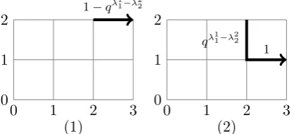
1. The 2 is inserted into the second row, pushing the existing second row over by

one: this outcome has weight 1−qλ11−λ22.

2. The 2 is inserted into the first row, pushing the existing 2’s over by one: this outcome has weightqλ11−λ22.

Note that these weights sum to one, as is always the case. The corresponding insertion paths, with edge weights indicated, are:

0 1 2 3

0 1

2 1−q

λ1₁−λ2₂

(1)

0 1 2 3

0 1 2

qλ1₁−λ2 2

1

(2)

The quantity λ1₁ −λ2₂ is the difference between the number of 1’s in the first row

and the number of 2’s in the second row, see Figure 2.2.

1 . . . 1 2 . . . 2

2 . . . 2 _λ1

[image:22.595.217.426.241.336.2]

1−λ22

Figure 2.2: The quantityλ1₁−λ2₂ in the exponent in Example 2

For example, inserting a 2 into

P = 1 1 2 2 2

gives

I2(P,P˜) =     

   

1−q if ˜P = ˜P2

q if ˜P = ˜P3

0 otherwise.

where

˜

P2 =

1 1 2 2

(23)

and

˜

P3 =

1 1 2 2 2

2 .

Example 3. Suppose l = 3. If we are inserting a 1 into P ∈ T₃ there is only one

possible outcome ˜P withI1(P,P˜)6= 0, namely the one obtained by the usual column insertion algorithm: the 1 is inserted into the first row, pushing the existing first

row over by one. The corresponding weighted insertion path is:

0 1 2 3 4

0 1 2 3

1 1 1

If we are inserting a 2, there are three possible outcomes:

1. The 2 is inserted into the second row, pushing the existing second row over by

one: this outcome has weight

(1−qλ11−λ22₎1−q λ2

1−λ32

1−qλ2 1−λ22

;

2. The 2 is inserted into the second row, bumping a 3 into the first row: this

outcome has weight

(1−qλ11−λ22₎ ₁−1−q λ2

1−λ32

1−qλ21−λ22 !

;

3. The 2 is inserted into the first row, pushing existing 2’s and 3’s in first row

(24)

The corresponding insertion paths, with edge weights indicated, are:

0 1 2 3 4

0 1 2 3

1−qλ1₁−λ2 2

1−qλ21−λ32 1−qλ21−λ22

(1)

0 1 2 3 4

0 1 2 3

1−qλ1₁−λ2 2

1−1−qλ2₁−λ3₂

1−qλ21−λ22

1

(2)

0 1 2 3 4

0 1 2 3

qλ1₁−λ2 2

1 1

(3)

If we are inserting a 3, there are also three possible outcomes: the 3 is placed in the third, second or first row with respective weights 1−qλ22−λ33_,_qλ22−λ33(1−_qλ21−λ32₎

andqλ22−λ33qλ21−λ32. The corresponding insertion paths, with edge weights indicated,

are:

0 1 2 3 4

0 1 2 3

1−qλ2₂−λ3 3

0 1 2 3 4

0 1 2 3

qλ22−λ33

1−qλ2₁−λ3 2

0 1 2 3 4

0 1 2 3

qλ2₂−λ3 3

qλ21−λ32

(25)

The quantitiesλ1₁−λ2₂,λ2₁−λ3₂, etc. which appear in the above weights are

illustrated in Figure 2.3.

1 . . . 1 2 . . . 2 3 . . . 3

2 . . . 2 3 . . . 3

3 . . . 3 λ1

1−λ22 λ21−λ32 λ2

[image:25.595.146.491.149.242.2]

2−λ33 λ21−λ22

Figure 2.3: The exponent quantities in Example 3.

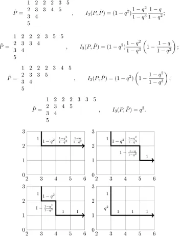
Example 4. Suppose we are inserting a 3 into

P =

1 2 2 2 3 5

2 3 4 5

3 4

5

(2.2)

The (four) possible output tableaux ˜P and their weights I3(P,P˜) are shown in

Figure 2.4, along with the corresponding weighted insertion paths.

The q-insertion algorithm can be applied to a word w = w1. . . wn ∈ [l]n,

starting with an empty tableau and successively inserting the numbersw1, w2, . . . , wn,

multiplying the weights along each possible sequence of output tableauxP(1), . . . , P(n) =

P to obtain a distribution of weights φw(P, Q) onTl× Sn. More precisely, we define

φw(P, Q) recursively as follows. Set

φk(P, Q) =  



1 ifP =kand Q= 1

0 otherwise.

Forw∈[l]n and ( ˜P ,Q˜)∈ T_l× Sn+1 with sh ˜P = sh ˜Q, define

φwk( ˜P ,Q˜) = X

φw(P, Q)Ik(P,P˜),

where the sum is over (P, Q)∈ T_l× S_n with shP = shQ.

We conclude this section by giving a more algorithmic description of theq -insertion algorithm. For this it is convenient to assume 0 ≤ q < 1 and describe

(26)

˜

P =

1 2 2 2 3 5

2 3 3 4 5

3 4

5

, I3(P,P˜) = (1−q2) 1−q2

1−q3 1−q

1−q2;

˜

P =

1 2 2 2 3 5 5

2 3 3 4

3 4

5

, I3(P,P˜) = (1−q2) 1−q2 1−q3

1− 1−q 1−q2

;

˜

P =

1 2 2 2 3 4 5

2 3 3 5

3 4

5

, I3(P,P˜) = (1−q2)

1−1−q 2

1−q3

;

˜

P =

1 2 2 2 3 3 5

2 3 4 5

3 4

5

, I3(P,P˜) =q2.

2 3 4 5 6

0 1 2 3

1

1−q2 1−q

2 1−q3

1−q

1−q2

2 3 4 5 6

0 1 2 3

1

1−q2 1−q

2 1−q3

1− 1−q

1−q2

1

2 3 4 5 6

0 1 2 3

1

1−q2

1−1₁−q_−q23

1 1

2 3 4 5 6

0 1 2 3 1 q2

[image:26.595.146.499.121.587.2]

1 1 1

Figure 2.4: The four possible output tableaux ˜P, their weights I3(P,P˜), and the corresponding insertion paths, with edge weights indicated, for k= 3 and P given by (2.2).

the language of ‘weights’ in the general case. For reference, we begin with an

(27)

1. Seti←1 and (P, Q) = (∅,∅).

2. Setk←wi and j←k.

3. If λk_j₋−₁1=λ_jk and j > 1 then set j ← j−1; otherwise k displaces the first number s in jth row of the tableau that is larger than k (s = ∞ and k is

appended at the end of the row if no such number exists) and setk←s.

4. If k = ∞ then append i to Q such that P and Q have the same shape, set

i←i+ 1 and go to step (2); otherwise go to step (3).

The q-insertion algorithim is defined as follows. We adopt here the following

con-vention: fori >0, let

qλi−0 1−λi1 =qλi0−λi1 =qλi0−λ

i−1 0 =qλ

i i−λ

i

i+1 =qλii−λ i−1

i =qλ i−1

i −λ i i+1 = 0.

This convention is used for covering boundary conditions in general arguments. It

is only used in the following description of the q-insertion algorithm as well as in Section 2.7.1. Otherwise the undefinedλi_j forj > i orj= 0 are taken to be zero.

1. Seti←1 and (P, Q) = (∅,∅).

2. Setk←wi,j←k,d←0 and ae(m, n)←fe(m, n) ∀e∈ {0,1},1≤n≤m.

3. With probability 1−ad(k, j) set j ←j−1 and d← 0; otherwise k displaces

the first number s injth row of the tableau that is larger thank(s=∞ and

append kat the end of jth row if no such number exists) and setk← sand

d←1.

4. If k = ∞ then append i to Q such that P and Q have the same shape, set

i←i+ 1 and go to step (2); otherwise go to step (3).

As is obvious, whenq= 0 it reduces to the usual column insertion algorithm.

2.4 Main result

The weightsφw(P, Q) are quite complicated. The main result of this chapter is that

a remarkable simplification occurs when we average over the set of words. Before

stating the result, we first introduce two more functions on tableaux and explain their connection toq-Whittaker functions and Macdonald polynomials. Denote the

q-Pochhammer symbol by

(28)

with the conventions (n)0 = (0)q= 1, and the q-binomial coefficients by " n m # q

= (n)q

(m)q(n−m)q

.

ForP ∈ T_l with shPi =λi, 1≤i≤l, writingλ=λl, define

κ(P) =

Ql−1 j=2

Qj−1 i=1(λ

j i −λ

j i+1)q Ql−1

j=1 Qj

i=1(λ j i −λ

j+1

i+1)q(λji+1−λ j i)q

= ∆l(λ)−1 Y

1≤j<i≤l "

λi_j −λi_j₊₁ λi

j−λi −1 j # q , where

∆l(λ) = l−1 Y

i=1

(λi−λi+1)q.

ForQ∈ S_n with shQi ₌_µi_{, 1}_≤_i_≤_n_{, define}

ρ(Q) = Y

1≤i≤j:µi j−µ

i−1

j =1

(1−qµij−µij+1₎_.

The functionsκand ρ are simply related as follows. Suppose that l≥nand P has

distinct entriesi1< i2 <· · ·< in. Denote by ˆP ∈ Snthe standard tableau obtained

by replacing the entryik by k, for each k= 1, . . . , n. Then

κ(P) = ρ( ˆP) (1−q)n_∆

l(λ)

. (2.3)

Indeed, using the simple identities,

"

a

0 #

q

= 1,

"

a

1 #

q

= 1−q

a

(29)

we have

κ(P) = ∆l(λ)−1 Y

1≤i<j≤l λi_j−λi−_j 1=1

"

λi_j −λi_j₊₁ λi

j−λi −1 j

#

q Y

1≤i<j≤l λi_j−λi−_j 1=0

"

λi_j−λi_j₊₁ λi

j−λi −1 j

#

q

= ∆l(λ)−1 Y

1≤i<j≤l λi

j−λ i−1

j =1

1−qλij−λij+1 1−q

Y

1≤i=j≤l λi

j−λ i−1

j =1

1−q

= ρ( ˆP) (1−q)n_∆

l(λ)

.

The functions κ and ρ are closely related to q-Whittaker functions [Rui90, Eti99, GLO10, GLO12]. Denote by Ωl the set of partitions with at most l parts.

Theq-Whittaker function with parameter a∈_Cl _{is a function on Ω}l _{defined by}

Ψa(λ) =

X

P∈Tl: shP=λ

aPκ(P). (2.5)

In [GLO11] it is shown that these functions are given in terms of the Macdonald

polynomialsPλ(x;q, t) as

Ψa(λ) = ∆l(λ)−1Pλ(a;q,0). (2.6)

From this it follows that

Ψa(λ) = ∆l(λ)−1 X

µ

kλµ(q)mµ(a) (2.7)

wheremµ denote the monomial symmetric functions and

kλµ(q) = ∆l(λ)

X

shP=λ,tyP=µ

κ(P) =X

ν

Kλν(q,0)Kνµ, (2.8)

where Kλµ(q, t) are the two-variable Kostka polynomials [Mac98]. We recall that

Kλν(q,0) =Kλ0_ν0(0, q) =K_λ0_ν0(q), where K_λµ(t) =K_λµ(0, t) are the single-variable

Kostka polynomials. For an extensive survey of the various properties and inter-pretations of these polynomials, see [Ana01]. When q = 0, κ(P) ≡ 1 and kλµ(0)

(30)

and typeµ. In this case, Ψa(λ) is given by the Schur polynomial

Ψa(λ) =sλ(a) = X

µ

Kλµmµ(a).

We will also consider the following functions:

fλ(q) = X

Q∈Sn: shQ=λ ρ(Q).

Note thatfλ(0) =fλ, the number of standard tableaux with shapeλ. The relation betweenfλ(q) and the Whittaker functions Ψais given by the following proposition,

which is a straightforward consequence of (2.3). Define

∆(λ) =

l(λ) Y

i=1

(λi−λi+1)q,

wherel(λ) denotes the number of parts inλ.

Proposition 5. For each λ`n,

lim

l→∞Ψ(1/l)l(λ) =

fλ(q)

n!(1−q)n_∆(_λ₎.

It follows, using

lim

l→∞sλ((1/l)

l_{) =}_fλ_/n_!_,

thatfλ(q) is also given, for λ`n, by

fλ(q) = (1−q)nX

µ

Kλµ(q,0)fµ.

To understand this in terms of specializations, recall that the exponential

special-ization ex1 is the homomorphism defined on the ring of symmetric functions by ex1(pn) =δn1, where pn are the elementary power sums (see, for example, [Sta01,

§7.8]). It follows from the above proposition (or can be seen directly) that

fλ(q) =n!(1−q)nex1(Pλ(q,0)).

(31)

Toda difference operators [Rui90, Rui99, Eti99, GLO10]. In particular,

LΨa= X

i

ai !

Ψa, (2.9)

whereL is the kernel operator defined by

L(λ, µ) =  



ci(λ) ifµ=λ+ei for some 1≤i≤l,

0 otherwise,

and

ci(λ) =  



1−qλi−λi+1+1 _{for 1}_≤_{i < l,}

1 fori=l.

Our main result is the following.

Theorem 6. Let (P, Q)∈ T_l× S_n with shP =shQ=λ. Then

X

w∈[l]n

φw(P, Q) = (λl)q−1κ(P)ρ(Q). (2.10)

We note the following immediate extension of this identity which is useful for applications. The type of a word w is the composition µ = (µ1, µ2, . . .) where

µi is the number of i’s in w. For a = (a1, . . . , al) and µ a composition, write

aµ =aµ1 1 . . . a

µl

l ; for w ∈ [l]n and P ∈ Tl, write aw = aty(w) and aP = atyP. Now,

sinceφw(P, Q) = 0 unless tyP = ty(w), we can write

X

w∈[l]n

awφw(P, Q) = (λl)q−1aPκ(P)ρ(Q). (2.11)

Summing (2.11) overP and Qgives

X

(P,Q)∈Tl×Sn:shP=shQ=λ

X

w∈[l]n

awφw(P, Q) = (λl)q−1Ψa(λ)fλ(q).

Note that this implies the Cauchy-Littlewood type identity

X

λ`n

(λl)−q1Ψa(λ)fλ(q) = X

i

ai !n

.

Theorem 6 also yields some combinatorial formulas.

(32)

shape λ. Then

Pλ(a;q,0) = X

w∈[l]n

HQ(w)aw

and

kλµ(q) =

X

w∈[l]n_:_ty₍_w₎₌_µ

HQ(w),

where

HQ(w) =

∆(λ)

ρ(Q) X

P

φw(P, Q).

Similarly, for any fixed P ∈ T_l with shape λ`n,

fλ(q) = X

w∈[l]n

GP(w),

where

GP(w) =

(λl)q

κ(P) X

Q

φw(P, Q).

Taking P to be standard with shape λ`n, this last formula becomes

ex1(Pλ(q,0)) =

1

n! X

σ∈Sn

HP(σ),

where the sum is over permutations andHP(σ) indicates the functionHP evaluated

at the word σ−1(1). . . σ−1(n).

When q = 0, HS(w) equals 1 if the Q-tableau obtained by applying the

Robinson-Schensted algorithm with column insertion to w is S, and 0 otherwise;

similarly, GT(w) equals 1 if the P-tableau obtained by applying the

Robinson-Schensted algorithm with column insertion towisT, and 0 otherwise. The functions

GT andHSthus generalise the notions ofP-equivalence andQ-equivalence, or Knuth

and dual Knuth equivalence, for the Robinson-Schensted algorithm with column

insertion (see, for example, [Ful97, Chapter 2 and§A.3]).

The key ingredient in the proof of Theorem 6 in Section 2.7.1 is the following

intertwining relation. Define kernel operatorsK and M by

K(λ, P) =aPκ(P)IshP=λ, M(P,P˜) = l X

k=1

(33)

Proposition 8. The following intertwining relation holds:

KM =LK (2.12)

We remark that (2.12) immediately yields the eigenvalue equation (2.9).

2.5 Stochastic evolutions

If 0≤q <1 anda∈_Rl + with

P

iai= 1, then

X

w∈[l]n

awφw(P, Q) = (λl)q−1aPκ(P)ρ(Q) (2.13)

defines a probability measure onT_l×S_n, which can be interpreted as the distribution

of the pair of tableaux obtained when one applies the randomised insertion algotihm to a random word w1. . . wn with each wi chosen independently at random from

[l] according to the probabilities a1, . . . , al. If we denote by L(m) the shape of

the tableau obtained after inserting the first m entries w1. . . wm then, given the

interpretation ofQ as a recording tableau, we conclude by summing (2.13) over P

that the sequence of shapesL(1), . . . ,L(n) is distributed according to

P(L(1) =µ1, . . . ,L(n) =µn) = (µn`) −1

q Ψa(µn)ρ(Q),

whereQ∈ S_n is defined by shQi=µi,i= 1, . . . , n. But this can be written as

P(L(1) =µ1, . . . ,L(n) =µn) =

n Y

i=1

Ψa(µi)

Ψa(µi−1)

L(µi−1, µi).

Since n is arbitrary, we immediately conclude the following. Write µ % λ if λ is

obtained from µby adding a single box.

Theorem 9. When applying the randomised insertion algorithm to a random word

w1w2. . . with each wi chosen independently at random from [l] according to the

probabilities a1, . . . , al the sequence of tableaux P(n), n ≥ 0 obtained evolves as a

Markov chain inT_l with transition probabilities

M(P,P˜) =

n X

k=1

akIk(P,P˜).

(34)

tran-sition probabilities

p(µ, λ) = Ψa(λ) Ψa(µ)

L(µ, λ)Iµ%λ.

The conditional law of P(n), given{L(1), . . . ,L(n); L(n) =λ}, is

P(P(n) =P| L(1), . . . ,L(n); L(n) =λ) = K(λ, P)

Ψa(λ)

.

The conditional law of tyP(n), given {L(1), . . . ,L(n); L(n) =λ}, is

P(tyP(n) =µ| L(1), . . . ,L(n); L(n) =λ) = a

µ_k λµ(q)

Ψa(λ)

.

The distribution of L(n) is given by

ν(λ) :=P(L(n) =λ) = (λl)q−1Ψa(λ)fλ(q).

The probability distribution ν is a particular specialisation (and restriction

toλ `n) of the Macdonald measures introduced by Forrester and Rains [PJF02],

see also [BC13]. When q = 0, the above theorem reduces to the fact [O’C03a] that, when applying the usual column insertion algorithm to a random word with

probabilities a1, . . . , al, the shape of the tableau evolves as a Markov chain with

transition probabilities

p(µ, λ) = sλ(a)

sµ(a)Iµ%λ

.

Ifa1 > a2 >· · ·> al this Markov chain can be interpreted as a random walk inNl

with transition probabilities

r(µ, λ) =aλ−µIµ%λ

conditioned never to exit the Weyl chamber{λ∈_Nl_: _λ

1 ≥ · · · ≥λl}, which can be

identified with Ωl. This result, which relates to the representation theory ofgl_l, has been generalised to arbitrary complex semisimple Lie algebras in [BBO05, LLP12].

For earlier related work on the asymptotics of longest monotone subsequences in random words, see [TW01]. When q → 1 the q-Whittaker functions converge

with appropriate rescaling to gl_l-Whittaker functions [GLO12], and the above the-orem should re-scale to the main result of the paper [O’C12], which relates a continuous-time version of the geometric RSK correspondence introduced by A.N.

Kirillov [Kir01], with Brownian motion as input, to the open quantum Toda chain

(35)

an appropriate sense to the continuous-time version of the geometric RSK mapping

considered in [O’C12], which is deterministic. The results of [O’C12] have been generalised in [Chh13] (see also [BBO09]) to arbitrary complex semisimple Lie

al-gebras. It is natural to expect the results of the present chapter to admit a similar

generalisation.

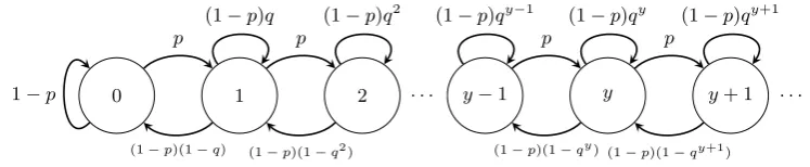
Example 10. The rank-1 case (l= 2) of Theorem 9 is discussed in [O’C14]. Setting Li₍_n_{) = shP}i₍_n_{), the evolution on tableaux in this case is driven by the process}

Y(n) = L1

1(n)− L21(n), n≥0, which (setting p=a1) is a birth and death process as illustrated in Figure 2.5.

0 1 2 y−1 y y+ 1

1−p

p p

. . .

p p

. . .

(1−p)(1−q) (1−p)(1−q2) (1−p)(1−qy) (1−p)(1−qy+1₎

[image:35.595.131.505.275.352.2]

(1−p)q (1−p)q2 (1−p)qy−1 (1−p)qy (1−p)qy+1

Figure 2.5: The birth-and-death process Y

Example 11. Whenl= 3 the algorithm is more complicated than in thel= 2 case

because the push-or-bump probability f1(3,2) appears. In this case the algorithm with random input is described as follows (cf. Example 2). In the following, w.p.

means “with probability”.

• w.p. a1, insert 1 to row 1, pushing 2’s and 3’s in row 1

• w.p. a2, insert 2

– w.p. 1−qλ11−λ22, the 2 is inserted to row 2 and the displaced 3 is either

pushed or bumped

∗ w.p. (1−qλ21−λ32)/(1−qλ21−λ22) the displaced 3 is pushed in row 2

∗ w.p. 1−(1−qλ21−λ32)/(1−qλ21−λ22) the displaced 3 is bumped to row

1

– w.p. qλ11−λ22, the 2 is inserted to row 1 and it pushes 3’s in row 1

• w.p. a3, insert 3

– w.p. 1−qλ22−λ33, the 3 is inserted to row 3

(36)

– w.p. qλ22−λ33qλ21−λ32 the 3 is inserted to row 1

Theq-insertion algorithm applied to a random word is closely related to the

q-TASEP interacting particle system. This is a variation of the totally asymmetric simple exclusion process (TASEP) which was introduced (in the language of q

-bosons) and shown to be integrable by Sasamoto and Wadati [SW98], and recently

related to q-Whittaker functions by Borodin and Corwin [BC13]. The process is defined as follows. There are l particles on the integer lattice, and we denote their

positions byx1> x2 >· · ·> xl. Let a1, a2, . . . , al ∈R+. Without loss of generality

we can assumeP

iai= 1. The particles jump independently to the right by 1 with

respective rates

ri=  



a1, ifi= 1;

ai(1−qxi−1−xi−1), otherwise.

Note that when xi + 1 = xi−1 the rate ri vanishes, thus enforcing the exclusion

rule. Now consider the tableau-valued Markov chain P(n), n ≥ 0, defined as above by applying the randomised insertion algorithm applied to a random word

with probabilities a1, . . . , al. Setting Li(n) = shPi(n), we see that the process

X1(n), . . . , Xl(n), n≥0 defined byXi(n) =Lii(n)−i+ 1 evolves as a Markov chain

with state space{x∈_Zl_: _x

1 > x2>· · ·> xl} and transition probabilities

π(x, x+ei) =ri, i= 1, . . . , l π(x, x) = 1− X

i

ri,

where ri are defined as above. In other words, it is a de-Poissonisation of the q

-TASEP process. Denote the q-TASEP process by ˜X(t), t ≥ 0, started with step initial condition ˜Xi(0) = 1−i,i= 1, . . . , l; by Theorem 9, the law of the position

of the last particle at timetis given by

P( ˜Xl(t) =m−l+ 1) = X

k≥0

e−tt

k

k! X

λ`k,λl₌_m

(λl)−q1Ψa(λ)fλ(q)

=e−t X

λ∈Ωl_,λ l=m

t|λ|

|λ|!(λl)

−1

q Ψa(λ)fλ(q). (2.14)

In [BC13], a continuous-time Markov chain on the set of tableaux T_l (actually

dis-crete Gelfand-Tsetlin patterns, but this is equivalent) was introduced. It has the same fixed time marginals as the Poissonisation of the processP(n), although the

(37)

q-TASEP process and in the paper [BC13] an equivalent expression to (2.14) is

ob-tained via this coupling for the law of ˜Xl(t). See also [BCS14] for related recent

work.

2.6 Permutations

Ifl=nand P ∈ Sn with shP =λ, then (2.3) becomes

κ(P) = ρ(P) (1−q)n_∆

n(λ)

.

Using this, and the fact that φw(P, Q) = 0 unless tyP = tyw, we immediately

deduce from Theorem 6 the following corollary.

Corollary 12. For P, Q∈ S_n with shP =shQ=λ, we have

ζP,Q(q) := X

σ∈Sn

φσ(P, Q) =

ρ(P)ρ(Q)

(1−q)n_∆(_λ₎. (2.15)

Summing overP andQ gives

θλ(q) :=

X

P,Q∈Sn:shP=shQ=λ

ζP,Q(q) =

fλ(q)2 (1−q)n_∆(_λ₎.

We note that P

λ`nθλ(q) = n!. When 0 ≤ q < 1, the probability measure on

integer partitions defined by µq(λ) = θλ(q)/n! gives the law of the shape of the

tableaux obtained when one applied the randomised insertion algorithm to a random

permutation. It would be interesting to understand the analogue in this setting of the longest increasing subsequence problem [AD99, BDJ99, Oko01].

For any standard tableauP with entries in [n] and shape λ, its weight ρ(P)

is a product ofnpolynomials of the form of (1−qk) and hence ρ(P) is divisible by (1−q)n. On the other hand, considering the ith and i+ 1th row in P, each time

j a box is added in ith row, a factor (1−qd) - where d is the difference between length of the corresponding two rows at timej- appears inρ(P). For this difference

dto reach the value of λi−λi+1 eventually (which it evidently does) all the factors

(1−q),(1−q2), . . . ,(1−qλi−λi+1_{) must appear at least once. It follows that} _ρ₍_P₎ is also divisible by ∆(λ). Thus,ζP,Q(q)∈Z[q] for each pair (P, Q) andθλ(q)∈Z[q]

for eachλ.

For any permutationσ∈Sn, denote by (P(σ), Q(σ)) the pair of tableaux

(38)

Fσ(q) andθλ(q) are given by

F12(q) = 1−q; F21(q) = 1 +q.

θ2(q) = 1 +q; θ12(q) = 1−q.

Whenn= 3, we have

F123(q) = (1−q)2; F132(q) = 1−q; F213(q) = (1 +q)(1−q2);

F231(q) = 1−q2; F312(q) = 1−q2; F321(q) = (1 +q)(1 +q+q2).

θ3(q) = (1 +q)(1 +q+q2); θ21(q) = (1−q)(2 +q)2; θ13(q) = (1−q)2.

The polynomials Fσ(q) give an alternative interpretation of the probability

measure µq as the distribution of the shape of the tableaux obtained when one

applies the Robinson-Schensted column insertion algorithm to a permutation chosen

at random according to the distributionFσ(q)/n!.

2.7 Proofs

2.7.1 Proof of Proposition 8

To prove (2.12), we take advantage of the recursive structure of the q-Whittaker functions. Define ˆκ on Ωl×Ωl−1 by

ˆ

κ(λl, λl−1) =

Ql−2 i=1(λ

l−1 i −λ

l−1 i+1)q Ql−1

i=1(λl −1

i −λli+1)q(λli−λl −1 i )q

and set

T ={(λl, λl−1)∈Ωl×Ωl−1 :λl−1 ≺λl},

where we writeλ≺µ ifµi+1≤λi ≤µi for each i.

We begin by verifying the simpler intertwining relation:

ˆ

(39)

where ˆM :T ×T →_R≥0 and ˆK :T →R≥0 are defined as follows.

ˆ

M((λl, λl−1),(λl+ek, λl−1)) =al(1−qλ

l−1

k−1−λ

l k₎

l−1 Y

i=k

qλl−i 1−λ l

i+1, 1≤k≤l;

ˆ

M((λl, λl−1),(λl+ek, λl−1+ek)) =

(1−qλl−k 1−λ l−1

k+1+1₎₍₁−_qλ

l−1

k−1−λlk₎

1−qλl−k−11−λ

l−1

k

,

1≤k≤l−1;

ˆ

M((λl,λl−1),(λl+ek, λl−1+em))

= (1−q

λml−1−λml−+11 +1₎₍₁−_qλlm−λ l−1

m ₎

1−qλl−m−11−λ

l−1

m

(1−qλl−k−11−λlk₎

m Y

i=k+1

qλl−i−11−λli_,

1≤k < m≤l−1.

ˆ

K(λl,(˜λl, λl−1)) =aPli=1λli− Pl−1

i=1λ

l−1

i ˆκ(λl, λl−1)_I

λl_=˜_λl.

With a slight abuse of notation we will write ˆK(λl, λl−1) as shorthand for ˆK(λl,(˜λl, λl−1))

since the support of latter is in{λl= ˜λl}. We’ll do the same for kernel K.

We will verify the recursive intertwining relation (2.16) directly. The left

hand side is given by

ˆ

KMˆ(λl,(λl+ek, λl−1)) = ˆK(λl, λl−1) ˆM((λl, λl−1),(λl+ek, λl−1))

+ ˆK(λl, λl−1−ek) ˆM((λl, λl−1−ek),(λl+ek, λl−1))Ik≤l−1

+

l−1 X

m=k+1 ˆ

K(λl, λl−1−em) ˆM((λl, λl−1−em),(λl+ek, λl−1))Ik≤l−2.

We calculate each term separately. SetK0 =alKˆ(λl, λl−1).

ˆ

K(λl, λl−1) ˆM((λl, λl−1),(λl+ek, λl−1)) =K0(1−qλ

l−1

k−1−λlk₎

l−1 Y

i=k

(40)

ˆ

K(λl,λl−1−ek) ˆM((λl, λl−1−ek),(λl+ek, λl−1))

=K0(1−q

λl−_k−1₁−λl−_k 1+1₎₍₁₋_qλl−_k 1−λl k+1₎

(1−qλl−k 1−λ l−1

k+1₎₍₁−_qλlk−λ l−1

k +1)

(1−qλl−k 1−λ l−1

k+1₎₍₁−_qλ

l−1

k−1−λlk₎

1−qλl−k−11−λ

l−1

k +1

=K0(1−qλk−l−11−λlk₎1−q

λl−_k 1−λl k+1

1−qλlk−λ l−1

k +1 .

l−1 X

m=k+1 ˆ

K(λl,λl−1−em) ˆM((λl, λl−1−em),(λl+ek, λl−1))

=K0

l−1 X

m=k+1

(1−qλl−m−11−λ

l−1

m +1₎₍₁₋_qλl−m1−λlm+1₎

(1−qλl−m1−λl−m+11 ₎₍₁−_qλlm−λ l−1

m +1₎

×(1−q

λml−1−λml−+11 )(1−qλlm−λ l−1

m +1₎

1−qλl−m−11−λ

l−1

m +1

(1−qλl−k−11−λ

l k₎

m Y

i=k+1

qλl−i−11−λ

l i

=K0(1−qλl−k−11−λ

l k₎

l−1 X

m=k+1

(1−qλl−m1−λlm+1₎ m Y

i=k+1

qλl−i−11−λli_.

The left hand side of (2.16) is thus given by

LHS=K0(1−qλl−k−11−λ

l k₎

l−1 Y

i=k

qλl−i 1−λ l i+1

+

l−1 X

m=k+1

(1−qλl−m1−λlm+1) m Y

i=k+1

qλl−i−11−λ

l i_I

k≤l−2+

1−qλl−k 1−λ l k+1

k +1 Ik≤l−1

!

=K0(1−qλk−l−11−λlk₎1−q

λl

k−λlk+1+1

k +1 .

The right hand side is much easier to calculate:

LKˆ(λl,(λl+ek, λl−1)) =L(λl, λl+ek) ˆK(λl+ek, λl−1)

=K0(1−qλlk−λ l

k+1+1₎ 1−q

λl−_k−1₁−λl k

1−qλl_k−λl−_k 1+1,

as required.

We will now prove (2.12) by induction on l. When l = 2, since ˆM2 is the

kernel for the whole tableau, the recursive intertwining relation (2.16) is equivalent to the full intertwining relation (2.12). Suppose the statement of the proposition

(41)

we have

Kl(λl, λ1:l−1) =Kl−1(λl−1, λ1:l−2) ˆKl(λl, λl−1). (2.17)

By the recursive nature of definition of φw, Ml can be expressed in terms of ˆMl,

Ml−1 andLl−1:

Ml(λ1:l,λ˜1:l) =I_λl−1_=˜_λl−1Mˆl((λl, λl

−1₎_,_(˜_λl_,_˜_λl−1₎₎

+I_λl−1_%_λ˜l−1

Ml−1(λ1:l−1,λ˜1:l−1)

Ll−1₍_λl−1_,_λ˜l−1₎ ˆ

Ml((λl, λl−1),(˜λl,λ˜l−1)).

For partitionsλ, µwrite λ µto mean that eitherλ=µorλ%µ. Then

KlMl(λl,(˜λl, λ1:l−1)) = X ˜

λ1:l−1_:˜_λl−1 _λl−1

Kl(λl,λ˜1:l−1)Ml((λl,λ˜1:l−1),(˜λl, λ1:l−1))

= X

˜ λ1:l−1

ˆ

Kl(λl,λ˜l−1)Kl−1(˜λl−1,˜λ1:l−2)I˜_λl−1₌_λl−1Mˆl((λl,˜λl

−1₎_,_(˜_λl_{, λ}l−1₎₎

+I˜_λl−1_%_λl−1

Ml−1(˜λ1:l−1, λ1:l−1)

Ll−1_(˜_λl−1_{, λ}l−1₎ ˆ

Ml((λl,λ˜l−1),(˜λl, λl−1))

=:I˜_λl−1₌_λl−1I +I_λ˜l−1_%_λl−1II.

II = X

˜

λl−1_%_λl−1 ˆ

Kl(λl,˜λl−1) ˆMl((λl,λ˜l−1),(˜λl, λl−1))

× X

˜

λ1:l−2_:˜_λl−2 _λl−2

Kl−1(˜λl−1,λ˜1:l−2)M

l−1_(˜_λ1:l−1_{, λ}1:l−1₎

Ll−1_(˜_λl−1_{, λ}l−1₎ !

= X

˜

λl−1_%_λl−1 ˆ

Kl(λl,˜λl−1) ˆMl((λl,λ˜l−1),(˜λl, λl−1))

×K

l−1_Ml−1_(˜_λl−1_,₍_λl−1_{, λ}1:l−2₎₎

Ll−1_(˜_λl−1_{, λ}l−1₎

!

induction ========

assumption

X

˜

λl−1_%_λl−1 ˆ

Kl(λl,λ˜l−1) ˆMl((λl,λ˜l−1),(˜λl, λl−1))

×L

l−1_Kl−1_(˜_λl−1_,₍_λl−1_{, λ}1:l−2₎₎

Ll−1_(˜_λl−1_{, λ}l−1₎

!

= X

˜

λl−1_%_λl−1 ˆ

(42)

Due to the indicator, when ˜λl−1 =λl−1,

I = ˆKl(λl,λ˜l−1)Kl−1(λl−1, λ1:l−2) ˆMl((λl,˜λl−1),(˜λl, λl−1)).

Therefore

KlMl(λl,(˜λl, λ1:l−1))

= X

˜

λl−1_:˜_λl−1 _λl−1 ˆ

Kl(λl,˜λl−1)Kl−1(λl−1, λ1:l−2) ˆMl((λl,˜λl−1),(˜λl, λl−1))

=Kl−1(λl−1, λ1:l−2) ˆKlMˆl(λl,(˜λl, λl−1))

(2.16)

= Kl−1(λl−1, λ1:l−2)Ll(λl,λ˜l) ˆKl(˜λl, λl−1)

(2.17)

= Ll(λl,˜λl)Kl(˜λl, λ1:l−1) =LK(λl,(˜λl, λ1:l−1)),

as required.

2.7.2 Proof of Theorem 6

We will prove the identity (2.11), from which the statement of the theorem follows.

From the definition of φw, for (P, Q) ∈ Tl × Sn such that shP = shQ = λ and

µi = shQi fori= 1, . . . , n, the left hand side of (2.11) can be written as

X

w∈[l]n

awφw(P, Q)

= X

w∈[l]n

X

(P(i))_in−₌₁1,shP(i)=µi

awIw1(∅, P(1)). . . Iwn(P(n−1), P)

= X

w∈[l]n

X

(aw1Iw1(∅, P(1))). . .(awnIwn(P(n−1), P))

= X



 X

w1∈[l]

aw1Iw1(∅, P(1)) 

. . . 

 X

wn∈[l]

awnIwn(P(n−1), P)





= X

M(∅, P(1)). . . M(P(n−1), P).

(43)

relation (2.12),

aPκ(P)ρ(Q) (λl)q

=L(∅, µ1). . . L(µn−1, λ)K(λ, P)

=L(∅, µ1). . . L(µn−2, µn−1)LK(µn−1, P)

=L(∅, µ1). . . L(µn−2, µn−1)KM(µn−1, P)

= X

P(n−1): shP(n−1)=µn−1

L(∅, µ1). . . L(µn−2, µn−1)

×K(µn−1, P(n−1))M(P(n−1), P) !

= X

P(n−1),P(n−2): shP(n−1)=µn−1_,_sh_P₍_n₋₂₎₌_µn−2

L(∅, µ1). . . K(µn−2, P(n−2))

×M(P(n−2), P(n−1))M(P(n−1), P) !

=· · ·= X

(P(i))n−_i₌₁1: shP(i)=µi

L(∅, µ1)K(µ1, P(1))M(P(1), P(2))×

· · · ×M(P(n−1), P) !

.

Now, from the definition of L, K and M, for P(1) ∈ T_l that has only one entry k

and whose shape isµ1 _{= (1),}

L(∅, µ1) = 1; K(µ1, P(1)) =M(∅, P(1)) =ak.

This completes the proof.

2.7.3 Proof of Proposition 5

Letλ`nand note that, forl > n, ∆l(λ) = ∆(λ). We want to show that

lim

l→∞Ψ(1/l)l(λ) =

fλ(q)

(44)

From the definition of Ψa, this is equivalent to

lim

l→∞l

−n X

P∈Tl: shP=λ

κ(P) = f

λ₍_q₎

n!(1−q)n_∆(_λ₎.

Write

X

P∈Tl: shP=λ

κ(P) =A+B

where A denotes the sum over tableaux with distinct entries and B denotes the

remaining sum. Assumel > n. By (2.3), if P has distinct entries, then

κ(P) = ρ( ˆP) (1−q)n_∆(_λ₎.

Hence

l−nA=l−n l n

! X

Q∈Sn

ρ(Q)

(1−q)n_∆(_λ₎ →

fλ(q)

n!(1−q)n_∆(_λ₎

as l → ∞. Thus it remains to show that l−nB → 0. We first show that κ(P) is bounded for P ∈ T_l with shP = λ. To see this, observe that if P has entries from

the set{i1, . . . , im} wherei1 <· · ·< im and ˜P denotes the tableau obtained from

P by replacing ik by k, for each k= 1, . . . , m, thenκ( ˜P) =κ(P). It follows that

κ(P)≤max

T∈Tn

κ(T)<∞.

Now, by the usual Robinson-Schensted correspondence, the number of P ∈ T_l with

shP =λwhich don’t have distinct entries is at most the number of words w∈[l]n which don’t have distinct entries, and this is given by

N(l, n) =ln− l

n

!

n!.

Robinson Schensted algorithms and quantum stochastic double product integrals

University of Warwick institutional repository:

http://go.warwick.ac.uk/wrap

A Thesis Submitted for the Degree of PhD at the University of Warwick

http://go.warwick.ac.uk/wrap/74169

This thesis is made available online and is protected by original copyright.

Please scroll down to view the document itself.

Robinson-Schensted algorithms and quantum

stochastic double product integrals

Yuchen Pei

Mathematics and Statistics Doctor Training Centre

Contents

Acknowledgments

Declarations

Abstract

Chapter 1

Introduction to

Robinson-Schensted algorithms

1.1

Overview

1.2

The classical Robinson-Schensted algorithms

1.3

The growth diagram

1.4

The dynamics of the RS algorithm taking a random

word

Chapter 2

A

q

-weighted

Robinson-Schensted algorithm

2.1

Introduction

2.2

The Robinson-Schensted algorithm

2.3

The

q

-weighted version

2.4

Main result

2.5

Stochastic evolutions

2.6

Permutations

2.7

Proofs