University of Warwick institutional repository:
http://go.warwick.ac.uk/wrap
A Thesis Submitted for the Degree of PhD at the University of Warwick
http://go.warwick.ac.uk/wrap/57476
This thesis is made available online and is protected by original copyright.
Please scroll down to view the document itself.
L I B R A R Y D E C L A R A T I O N A N D
D E P O S I T A G R E E M E N T
student details
Full name: . . . . University ID number: . . . .
thesis deposit
I understand that under my registration at the University, I am required to de-posit my thesis with the University in both hard copy and digital format.
The hard copy will be housed in the University Library. The digital version will be deposited in the University’s Institutional Repository (WRAP). Unless oth-erwise indicated, this will be made openly accessible on the Internet and will be supplied to the British Library to be made available online via its Electronic Theses Online Service (EThOS) service.
In exceptional circumstances, the Chair of the Board of Graduate Studies may grant permission for an embargo to be placed on public access to the hard copy thesis for a limited period. It is also possible to apply separately for an embargo on the digital version.
Hard Copy
I hereby deposit a hard copy of my thesis at the University Library to be made publicly available to readers immediately.
I agree that my thesis may be photocopied.
Digital Copy
I hereby deposit a digital copy of my thesis to be held in the WRAP and made available via the EThOS.
My thesis can be made publicly available online.
granting of non-exclusive rights
I agree to the following:
my thesis in its present version or future versions. I agree that the institutional repository administrators and the British Library or their agents may, without changing content, digitize and migrate my thesis to any medium or format for the purpose of future preservation and accessibility.
declarations
I declare that:
I am the author and owner of the copyright in my thesis and I have the authority of the authors and owners of the copyright in my thesis to make this agreement. Reproduction of any part of this thesis for teaching or in academic or other forms of publication is subject to the normal limitations on the use of copy-righted materials and to the proper and full acknowledgement of its source.
The digital version of my thesis I am supplying is the same version as the final, hardbound copy submitted in completion of my degree, once any minor correc-tions have been completed.
I have exercized reasonable care to ensure that my thesis is original, and does not to the best of my knowledge break any UK law or other intellectual property right, or contain any confidential material.
I understand that, through the medium of the Internet, my files will be avail-able to automated agents, and may be searched and copied by, for example, text mining and plagiarism detection software.
I grant the University of Warwick and the British Library a licence to make available on the Internet my thesis in digitized format through the Institutional Repository and through the British Library via the EThOS service.
If my thesis does include any substantial subsidiary material owned by third-party copyright holders, I have sought and obtained permission to include it in any version of my thesis available in digital format and that this permission encompasses the rights that I have granted to the University of Warwick and to the British Library.
legal infringements
I understand that neither the University of Warwick nor the British Library have any obligation to take legal action on behalf of myself, or other rights holders, in the event of infringement of intellectual property rights, breach of contract or of any other right, in my thesis.
B I O L O G I C A L L Y P L A U S I B L E
A T T R A C T O R N E T W O R K S
tristan james webb
thesis
submitted to the university of warwick
for the degree of
doctor of philosophy
complexity science doctoral training centre
department of computer science
C O N T E N T S
introduction xii
I
Background and Methods
1
1 attractor networks 2
1.1 Previous modeling work . . . 2
1.1.1 Two alternative forced choice decision-making models . . . 3
1.2 Artificial neurons . . . 4
1.2.1 Attractor network architecture . . . 6
1.3 Hopfield networks . . . 10
2 spiking neural network models 13 2.1 An integrate-and-fire attractor neuronal network model of decision-making: Methods used throughout the thesis . . . 17
II
Main Results
24
3 noise in attractor networks in the brain produced by graded firing rate representations 25 3.1 Methods . . . 273.1.1 Graded weight patterns . . . 27
3.2 Results . . . 29
3.2.1 Firing rate distribution . . . 29
3.2.2 Decision time . . . 31
3.2.3 Performance during decision-making with∆λ6=0 . . . 35
3.2.4 Stability of the spontaneous state . . . 36
3.2.5 Noise in the system: the variance of the firing rates of the neurons 37 3.2.6 Spectral analysis of decision pool power spectra . . . 39
3.2.7 Noise with graded representations in larger networks . . . 40
3.3 Discussion . . . 41
4 cortical attractor network dynamics with diluted connectivity 47 4.1 Methods . . . 48
4.1.1 Diluted connectivity . . . 48
4.2 Results . . . 51
4.2.1 Decision time . . . 51
4.2.2 Decision accuracy . . . 53
4.2.3 Stability of the spontaneous state . . . 53
4.2.4 Sparseness . . . 54
4.2.5 Performance with connectivity diluted to0.1. . . 54
4.2.6 Performance as a function of the input bias∆λ. . . 55
4.2.8 Noise in the system: within-trial variability . . . 57
4.3 Discussion . . . 58
5 communication before coherence 62 5.1 Introduction . . . 62
5.2 Methods . . . 63
5.2.1 Two network experiment design . . . 63
5.2.2 Analyses . . . 65
5.3 Results . . . 68
5.3.1 Information transmission between two coupled networks . . . . 68
5.3.2 Information transmission when the phase between two coupled networks is externally controlled . . . 78
5.4 Discussion . . . 79
6 discussion 85 6.1 Synfire chains . . . 85
6.2 Other sources of noise in the brain . . . 86
6.3 Contributions to understanding the stochastic functioning of the brain . . . 87
6.4 Contributions to the CTC hypothesis . . . 89
6.5 Possible future work . . . 92
6.5.1 Formation of graded weight patterns . . . 92
6.5.2 Other methods to generate coherence between networks . . . . 93
6.6 Conclusion . . . 93
L I S T O F F I G U R E S
Figure 1 Artist’s rendition of a typical neuron. . . xiii Figure 2 Illustration of the synaptic vesicle release cycle . . . . xiv Figure 3 The major components of an McCulloch-Pitts neuron 5 Figure 4 Connection diagram of an attractor network . . . 7 Figure 5 Firing of a recurrent McCulloch-Pitts neural network 9 Figure 6 Hodgkin-Huxley neuron simulation . . . 14 Figure 7 Effect of spiking input on a neuron’s membrane potential 16 Figure 8 The architecture of the probabilistic decision-making
spiking neural network. . . 21 Figure 9 Neuron recordings from primates show graded firing
rates . . . 26 Figure 10 Visualization of the graded weight matrix . . . 28 Figure 11 Average firing rates for the different pools on a single
trial . . . 29 Figure 12 Mean firing rates of individual neurons . . . 30 Figure 13 Firing rate probability distributions of the winning pool 31 Figure 14 Histograms of reaction times for graded and binary
firing rate distribution simulations . . . 32 Figure 15 Decision times of simulations with a shifted recurrent
weight parameter . . . 33 Figure 16 The percentage of trials on which the spontaneous state
was stable for networks of different size . . . 35 Figure 17 Decision times and percentage correct for networks of
different size . . . 36 Figure 18 Mean firing rates for the winning and losing pools . . 37 Figure 19 The distribution of the variance across trials of the
fir-ing rates of neurons in pool 1 durfir-ing the spontaneous period . . . 38 Figure 20 Power spectral densities and modulated power
spec-tral densities for the winning pool . . . 39 Figure 21 Visualization of the decision pool connectivity . . . . 50 Figure 22 Mean firing rates over trials in fully connected
net-works and netnet-works with diluted connectivity . . . . 51 Figure 23 Histograms of decision times for with full and diluted
connectivity . . . 52 Figure 24 Stability of the spontaneous firing state before the
de-cision cues are applied . . . 53 Figure 25 Decision time as a function of∆λfor networks with
full connectivity, and with diluted connectivities . . . 54 Figure 26 The Fano factors for the fully connected network and
for the networks with diluted connectivity . . . 56 Figure 27 Schematic representation of the network used to test
Figure 28 A single trial of the CTC simulation to illustrate the responses of the network in the AMPA case as a func-tion of time . . . 69 Figure 29 LFP frequency analyses for the AMPA case withwf =
0.45, the AMPA case withwf=0.021, and the NMDA
case . . . 70 Figure 30 Spectral analyses as a function of time for a single trial 72 Figure 31 Performance of the network as a function of the value
of the forward coupling weightwf . . . 75
Figure 32 Decision time for Net 2 as a function of the value of the forward coupling weightwf, the Cross-Spectral
L I S T O F T A B L E S
Table 1 Default parameter set . . . 19 Table 2 Parameters for the full and diluted connectivity
sim-ulations . . . 50 Table 3 The default parameter set used in the two network
A C K N O W L E G M E N T S
During the course of my Ph.D., there have been many people that have sup-ported and encouraged me. Without them, this thesis would not have been possible.
Foremost, I must thank my supervisors Jianfeng Feng and Edmund Rolls. I owe them both a great deal of inspiration. Professor Rolls in particular was very supportive of my work and a source of many ideas and feedback. It was a great learning experience to work alongside a scientist of his character. He has shown me the real importance and role that computational neuroscience will play in society. I feel very privileged to have had them both as my supervisors.
Dimitris Vavoulis has been a great friend, and the source of much conversa-tion about computaconversa-tional neuroscience and programming ideas. His friendship has certainly shaped the work I have done.
I thank all of my colleagues in the Complexity Science DTC, and Compu-tational Biology group. The community surrounding the DTC embodies an unique blend of theory and practice, and I am very pleased to have chosen it as the place to do my doctorate. I am also very grateful to the hardworking HPC staff at the University of Warwick for keeping our computing resources highly available.
P U B L I C A T I O N S
Rolls, E. T. and T. J. Webb (2011). “Cortical attractor network dynamics with diluted connectivity”.Brain Research1434, pp. 212–225.
Rolls, E. T. and T. J. Webb (2012). “Communication before Coherence”. Euro-pean Journal of Neuroscience, accepted.
A B S T R A C T
I N T R O D U C T I O N
T
he aim of this thesis is the study of stochastic neural networks for decision-making. The nervous systems consists of connected neural networks and is one of the most highly complex objects we have attempted to study in detail. There has been much progress in our theoretical understanding by using mathematics and dynamical systems theory as a basis to construct mod-els of neural function. However, to pursue greater insight into the functioning of the actual brain, we must incorporate a biological understanding into these models. This thesis will describe how such mathematical models have been ex-tended and simulated using techniques of computational neuroscience, so that they can be better applied to understanding brain function.problem background
The function of the brain, and its relationship to intelligence, has been under consideration for hundreds of years, and now the structure of the brain is much more understood than in any other point in history. Nevertheless, we are a very long way from a full understanding of of this complex structure. We describe here basic neurophysiology at the neuron level, because this is the basic level at which information is transmitted in the nervous system. I also present the idea here that in order to understand the network level, that is the level of large scale complex systems, we must consider it from the perspective of computational neuroscience. Here I describe the promising area of attractor networks.
Basic neurophysiology
The Italian scientist Galvani first observed frog legs jumping to life when ex-posed to electricity over 200 years ago, which opened the door for the empir-ical neuroscience by enlightening us to the electrophysiologempir-ical nature of the nervous system. The so-called age of the microscope that started in the 1800s al-lowed neuroscientists to be able to see the fine cellular makeup that dictates the brain’s functioning. The “neuron doctrine” posed by Cajal, among others, (Bul-lock et al., 2005) has been verified through years of experimental neuroscience, and we now know that the brain is made up of individual neurons which com-municate in a vast network through all or nothing electrical signals known as “action potentials”. Still, until recently, neuroscience has been struggling with the problem of cataloging the incredible molecular complexity throughout the brain. Shepherd (1988) states inNeurobiologythat
Today these discoveries form the basis of many mathematical models of brain function.
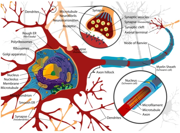
[image:14.595.148.461.242.474.2]The accepted understanding of a prototypical neuron is illustrated in Figure 1. Due to a careful balance of ions a neuron remains in an electrically polarized state from the surrounding inter-cellular fluid. Scientists such as Galvani were able to observe the affect an electrical stimulus had on a neuron, the generation of action potentials. When neurons fire naturally, the action potential impulse is very quick and can be thought of as a discrete event. Modelers can often think of these events as a “shot noise” and approximate the activity of a single action potential as a delta function. Once a neuron fires it reverts to a subthreshold state, and may remain in a refractory period in which it is less susceptible to input.
Figure 1:Artist’s rendition of a typical neuron. Electrical activity is generated along the axon as a result of the input from other neurons. Detail shows Mylina-tion of the Axon, which facilitates the speed of electrical impulses, and the connection points of neurons known as synapses.1
Of special interest to us is thesynapse, or the small gap present at the connec-tion between two neurons. Many of our recent investigaconnec-tions into molecular neurobiology have primarily been focused on categorizing the proteins respon-sible for neurotransmitter release at the synapse (Sudhof, 2004). The synaptic vesicle release cycle is the term used to describe the processes of communication that occurs at the synapse on the arrival of an electrical impulse, see Figure 2. We now know that this communication between neurons to be mediated by an electrochemical process. The chemicals released at synapse that signal an ac-tion potential are known as neurotransmitters. Their release is caused by Ca2+
intake when an action potential arrives at the presynaptic terminal.
1 Figure taken from http://en.wikipedia.org/wiki/File:Complete_neuron_cell_
In this thesis, I will be examining three of the major neurotransmitters present in the brain, AMPA, NMDA, and GABA. AMPA and NMDA are excitatory neu-rotransmitter receptors, that implement the effect of glutamate (Purves, 2007). AMPA and NMDA differ in the speed at which the chemical signal is propa-gated to the post-synaptic neuron, with AMPA mediated potentials being much faster than NMDA. GABA is primary inhibitory neurotransmitter in the brain (Watanabe and Maemura, 2002).
Figure 2:Illustration of the synaptic vesicle release cycle with neuron A transmitting to neuron B.2
Neurobiology of decision-making
What is the brain activity that is associated with making a decision, and what accounts for predictability of the choice? By decision-making, I refer to the pro-cess that we all go through when deciding an alternative between two or more choices. We have long known that this process is associated with an aspect of chance in the discrimination of stimuli (Thurstone, 1987). Tversky (1972) stated that "When faced with a choice among several alternatives, people often expe-rience uncertainty and exhibit inconsistency" and went on to develop a proba-bilistic framework of decision-making. These questions have recently lead to experiments involving recording brain activity, and they have highlighted a few key areas of the brain that may be involved. Here, I will review them to provide a justification of the model of decision-making I use in this thesis.
Key reviews of the neurobiology of decision-making have been produced by Gold and M. N. Shadlen (2007) and Schall (2001). The premise on which Gold and M. N. Shadlen (2007) argue is that somewhere in the brain are neurons spe-cialized to the task of encoding a decision. We can think of this activity as being represented by a decision vector (DV). Gold and M. N. Shadlen (2007) iden-tify this vector with all the internal “deliberations” that occur during a decision-making process, and assign it with a rule that signals the conclusion of decision. This approach leads to theories of decision making that can be verified by locat-ing the decision vector in neurological data.
The brain processes sensory information in many specialized brain areas. For instance, the main sensory brain area for the sense of touch is the primary so-matosensory cortex (S1) (Kandel, J. Schwartz, and Jessell, 2012). Neurons that are involved in the perception of vision during visual motion tasks have been found in the middle temporal (MT) area (K. Britten et al., 1993). These sensory areas are connected to areas of the brain that produces behavioral responses, such as the superior colliculus (SC), the lateral intraparietal area (LIP), and the frontal eye field (FEF), which all control eye movements (Schall, 2001).
Two perceptual tasks used in decision-making experiments are vibrotactile frequency discrimination (VTFD) and random dot motion (RDM). These ex-periments have been conducted alongside simultaneous recording of neurons using single- and multi-unit recording (Luna et al., 2005; Mountcastle, Stein-metz, and Romo, 1990; Romo and Salinas, 2003).
VTFD involves subjects discriminating between two flutter stimuli,f1and f2, applied to their fingertips (Li Hegner et al., 2009). These stimuli are
typi-cally in the5–50Hz range, and there is a short time gap between their
applica-tion. Work done by Romo and collaborators have found that neurons in S1 have firing rates that correspond to the frequency of each stimulus (Romo, Hernan-dez, and Zainos, 2004). It is not currently thought that neurons in S1 compare the two signals, because the neurons in S1 respond to bothf1andf2and they
do not seem to compute any stimulus comparison (Gold and M. N. Shadlen, 2007). Romo’s lab found that activity in the secondary somatosensory cortex (S2) and dorsolateral prefrontal cortex (dlPFC), but to greatest extent activity in the ventral premotor cortex (VPC) and medial premotor cortex (MPC) re-flected a comparison between the two stimuli (Hernandez, Zainos, and Romo, 2002; Romo, Brody, et al., 1999; Romo, Hernandez, and Zainos, 2004; Romo, Hernandez, Zainos, et al., 2002). The exact relationship between these different brain areas is still unknown, but these experiments have lead to proposed theo-retical frameworks of decision making where activity in S1 encodes the stimulus and the VPC and MPC neurons encode a probabilistic response (Deco and E. T. Rolls, 2006; Deco, E. T. Rolls, et al., 2012).
sen-sory information, in this case the area is the MT area (K. Britten et al., 1993; W. T. Newsome, K. H. Britten, and J. A. Movshon, 1989). The position of the LIP area in between the MT area and the SC and FEF areas lead researchers to focus on the LIP area as possible area to encode a DV (Gold and M. N. Shadlen, 2007). Neural activity in this area has been found to correspond to decision per-formance on a RDM task (M. Shadlen and W. Newsome, 1996; M. Shadlen and W. Newsome, 2001). In addition, reaction time versions of the RDM tasks have produced results that have been reproduced in theoretical models of decision-making (Ditterich, Mazurek, and M. Shadlen, 2003; Vandekerckhove and Tuer-linckx, 2007; X.-J. Wang, 2002)
The experimental work done by Romo and Shadlen have shaped recent re-search in decision-making. Recent experiments using fRMI data gathered from humans subjects has pointed at the neural correlates of the speed-accuracy trade off (Criss, Wheeler, and McClelland, 2012; Ivanoff, Branning, and Marois, 2008; Van Veen, Krug, and C. Carter, 2008). Future experiments may help us soon locate more of the signaling pathways involved in decision making.
Computational neuroscience
Determining the structure of biological neural networks has been a very difficult task due to the high density of brain tissue. For years scientists relied primarily on the microscope and electrophysiological techniques such as voltage-clamp experiments. These limitation have recently been lifting in recent years with new optical imaging techniques that can complement electrophysiological tech-niques (Scanziani and Häusser, 2009).
While molecular biologists have explored the brain at smaller scales, larger neural systems have been investigated using functional magnetic resonance imag-ing (fMRI), electroencephalography (EEG), magnetoencephalography (MEG), and multielectrode array (MEA) data. Bullmore and Sporns (2009) review how these experimental techniques are used to map the functional systems of the brain and offer explanations for behavior and cognition. This last point em-phasizes the need to synthesize the findings of experimental neuroscience with theory and computer simulations at the network level.
purely theoretical models or be used as data generating models that can be veri-fied with empirical results (EEG, MEG, MRI). All of this means, especially with the recent advances in gathering empirical results, computational neuroscience provides a theoretical means to model high-level traits, such as behavior and cognition, through models that have been devised from low level biological ob-servations.
Neural network theory has long been connected to the study of physical sys-tems and to associative memory syssys-tems in the brain (Little, 1974; Willshaw, Buneman, and Longuet-Higgins, 1969). Through work pioneered by John Hop-field, associative memory in neural networks was paralleled with statistical physics when he commented on an artificial neural network “This case is isomorphic with an Ising model” (Hopfield, 1982). Hopfield’s work went further than work previously done by formulating a Lyapunov function that accounted for the dy-namics of his network. This theory became a success because of the strong un-derstanding of the statistical mechanics available at the time. For example, it became possible to compute the memory capacity of a neural network using just the information about its microscopic properties (A. Treves and E. T. Rolls, 1991). Work conducted by Daniel Amit, Nicolas Brunel, and Xiao-Jing Wang has lead to a time dependent spiking attractor network framework model of the areas of the brain associated with decision-making known to exist in the cerebral cortex (Amit and Brunel, 1997a; X.-J. Wang, 2002). Work like this has shown that simple models of the nervous system possess many complex proper-ties. Feedback, an essential element of the actual nervous system, creates highly non-linear dynamics for these networks. In section 2.1, I describe a “balanced excitation-inhibition” network inspired by the work of Amit, Brunel, and Wang which is used for the computational modeling undertaken in this thesis.
In this thesis, I will be investigating the fundamental properties of the at-tractor network model and its biological significance. These networks can be used to model the functioning of the memory subsystems of the brain (B. Mc-Naughton and Morris, 1987; E. T. Rolls, 1996). Or they can provide a model for learning, such as how Pavlov’s classical conditioning may arise (Tesauro, 1986). Attractor networks have great explanatory power because stored memories can be recalled by a small fragment of that memory as a cue. The connections be-tween neurons are also governed by the biologically accepted associative, or Hebbian, learning, named after the observations of Donald Hebb in his book The Organization of Behavior(Hebb, 1949). Hebbian learning has been almost universally accepted as describing the modifications of synaptic strength associ-ated with long term potentiation (LTP), first experimentally observed by (Bliss and Gardner-Medwin, 1973), and its counterpart long term depression (LTD), discovered shortly afterwards by Lynch, Dunwiddie, and Gribkoff (1977).
of decision-making researched by other scientists, but such a contrast should not be perceived as negative one.
aim of this thesis
Seminal work done by many theoretical neuroscientists has grounded the field in well established branches of mathematics. Modern attractor network theory has been rooted in statistical physics since the work of Hopfield (1982). Hop-field’s contribution was deriving a model that used a Hebbian learning rule and also constructing a homeomorphism with the well known Ising model. Hop-field’s model is regarded as a milestone is stimulating interest in the field of at-tractor networks, even though outside of Hebbian learning and the basic attrac-tor network architecture it is not a biologically plausible model (Wilson, 2009). We shall see how models of spiking neurons, that have been studied as dynami-cal systems with a geometric interpretation by Rinzel (1986), among others, are used to make the basic notion of attractor networks more biologically plausible while still remaining true to the original theory. Furthermore, the biological abstractions in Hopfield networks allowed the proof of their ability to perform content addressable memory recall. The assumptions have made it easier to analyze these systems to determine quantities such as storage capacity using methods of statistical physics. We can therefore gauge the performance of an attractor network with a mean-field equivalent by knowing parameters such as connectivity, sparseness, and the memory pattern encoding. It is increasingly known the simplifications employed by Hopfield, such as assuming a binary firing distribution of neurons, may not apply in the brain. The distribution of neural firing rates in the brain is exponential (Baddeley et al., 1997; Franco et al., 2007; S. Treves A. P. et al., 1999), and the connectivity of neurons is diluted, with neurons in a given area connected to other local neurons with a value as low as 4% (Ishizuka, Cowan, and D. G. Amaral, 1995; Li et al., 1994; E. T. Rolls et al., 1997a).
Each of the chapters in turn will:
• Measure performance of realistic networks versus networks with mean-field equivalents.
• Quantify noise in biologically plausible neural networks.
• Test the Communication through Coherence Hypothesis using an attrac-tor network model.
organization of this thesis
This thesis is split into two main parts, the first part being a description of at-tractor models and the spiking neural network I use, and the second part being three chapters that comprise the original research of this thesis. What follows is a brief description of each chapter.
Attractor Networks
Attractor networks posses rich information processing abilities. I show how they posses properties needed for memory, learning, and decision-making.
Spiking Neural Network Models
A computational neuroscience model of decision-making is presented in Chap-ter 2. I examine the stochastic methods used in neuroscience to model spiking neural networks, and present the major models used in the field to simulate decision-making. Finally, I define the model used in Chapter 3, Chapter 4, and Chapter 5.
Graded Firing Rates in the Brain
In Chapter 3, I discuss how representations in the cortex are often distributed with graded firing rates in the neuronal populations. The firing rate probabil-ity distribution of each neuron to a set of stimuli is often exponential or gamma (Baddeley et al., 1997; Franco et al., 2007; S. Treves A. P. et al., 1999). In processes in the brain, such as decision-making, that are influenced by the noise produced by the close to random spike timings of each neuron for a given mean rate, the noise with this graded type of representation may be larger than with the bi-nary firing rate distribution that is usually investigated. In integrate-and-fire simulations of an attractor decision-making network, we show that the noise is indeed greater for a given sparseness of the representation for graded, exponen-tial, than for binary firing rate distributions. The greater noise was measured by faster escape times from the spontaneous firing rate state when the decision cues are applied, and this corresponds to faster decision or reaction times. The greater noise was also evident as less stability of the spontaneous firing state be-fore the decision cues are applied. The implication is that spiking-related noise will continue to be a factor that influences processes such as decision-making, signal detection, short-term memory, and memory recall even with the quite large networks found in the cerebral cortex. In these networks there are several thousand recurrent collateral synapses onto each neuron. The greater noise with graded firing rate distributions has the advantage that it can increase the speed of operation of cortical circuitry.
Diluted Connectivity
In Chapter 4, I discuss the role of dilution on spiking related noise in the cortex. The connectivity of the cerebral cortex is diluted, with the probability of excita-tory connections between even neighboring pyramidal cells rarely more than
0.1, and in the hippocampus0.04(Ishizuka, Cowan, and D. G. Amaral, 1995;
Li et al., 1994; E. T. Rolls et al., 1997a). To investigate the extent to which this diluted connectivity affects the dynamics of attractor networks in the cerebral cortex, I simulated an integrate-and-fire attractor network taking decisions be-tween competing inputs with diluted connectivity of0.25or0.1but the same
number of synaptic connections per neuron (80) for the recurrent collateral
The decision times were a little slower with diluted than with complete connec-tivity (full connecconnec-tivity894ms,0.25dilution940ms, and0.1dilution1,013
ms). The accuracy of the correct decisions (with∆λ=6.4) increased with
dilu-tion: full connectivity64.3%,0.25dilution75.7%, and0.1dilution90.3%. The
stability of the network when in the spontaneous state of firing was increased by dilution: full connectivity11.4%of trial were unstable,0.25dilution0.8%
of trials, and0.1dilution0%of trials. Given that the capacity of the network
is set by the number of recurrent collateral synaptic connections per neuron, on which there is a biological limit, the findings indicate that the stability of cortical networks, and the accuracy of their correct decisions or memory recall operations, can be increased by utilizing diluted connectivity and correspond-ingly increasing the number of neurons in the network, with little impact on the speed of processing of the cortex. Thus, diluted connectivity can decrease cortical spiking-related noise.
Communication through Coherence
In Chapter 5, I test the Communication through Coherence Hypothesis. The communication through coherence hypothesis proposes that coherent or syn-chronous oscillations in connected neural systems can promote communica-tion. I tested this in an integrate-and-fire network in which one network was connected to a second network by synaptic connection strengths that were sys-tematically increased in strength in different simulations. Each of the networks was an attractor decision-making network, and the decision populations of neu-rons of the two networks were connected by associative connections such that a decision in the first network could, trigger a corresponding decision in the second network. Gamma oscillations could be induced by increasing the rel-ative conductance of AMPA to NMDA excitatory synapses. It was found that very small connection strengths between the networks were sufficient to pro-duce information transmission (measured by Shannon mutual information) such that the second network took the correct decision based on the state of the first network. Although gamma oscillations were present in both networks, the synaptic connections sufficient for perfect information transmission (100
percent correct,1bit of transmitted information) were insufficiently strong to
produce coherence, phase locking or dependency, between the two networks, which only occurred when the synaptic strengths were increased more than10
Part I
1
A T T R A C T O R N E T W O R K S
I
n this chapter I will consider how simple neural networks models can func-tion as memory systems. The namesattractor network,autoassociator net-work, andassociative memory networkall basically refer to the same thing; that is a neural network with enough feedback to provide itself with a tendency to settle in to a steady firing pattern, the attractor state (Eliasmith, 2007). At-tractor networks came to be thought of as a type of memory system that would offer content addressing. This means that the network will reconstruct a stored memory, in the form of an attractor state, if it given an initial partial cue. This ability of attractor networks makes them likely to be involved in representing memory in the nervous system. It is theorized that these networks store pat-terns or memories for subsequent retrieval through the strength, or weight, of synapses (Amit, 1989).1.1
previous modeling work
Attractor networks have been implicated as a basic building block of large scale neural networks, such as the thalamus and hippocampus (Rinzel et al., 1998), In the hippocampus, Buzsáki (1997) has suggested that it is an attractor network ar-chitecture that is responsible for the theta oscillations that have been observed through EEG recordings. The CA3 region of the hippocampus has been shown to posses the same feedback architecture that characterizes attractor networks (D. Amaral and Witter, 1989). The neurons in the CA3 region have both highly collateralized and spatially extensive axons that are connecting to other CA3 neurons in what are known as the associative projections (D. G. Amaral, 1993). In a rat study, Ishizuka, Cowan, and D. G. Amaral (1995) found that the CA3 dendritic trees contained a systematic variation in the dendritic length and pro-portion of the dendritic tree in other areas of the hippocampus as a function of the location of the cell in the CA3 region.
spontaneous activity. In experimental studies, bothin vivoandin vitro, of these default states, neuron firing patterns show a temporal progression of activity that is similar to that observed when the area is exposed to stimulation (Luczak and MacLean, 2012).
It has been theorized that this architecture lets the CA3 system function as a single network with an approximate connectivity of4% between CA3 cells (A.
Treves and E. T. Rolls, 1994b). Many similar models that account for the storage of episodic memory in the hippocampus by the steady activation of cells in an attractor network have been suggested (B. L. McNaughton et al., 1996; O’Reilly and McClelland, 1994; E. T. Rolls, 2008). Another account of hippocampal func-tion has stemmed from early work by O’Keefe and Nadel (1978) which discov-ered that the hippocampus contains place cells that seem to encode a cognitive map of an animal’s environment. Lisman (2005) has suggested that hippocam-pal memory sequences are encoded in theta and gamma frequency oscillations that cue off the firing of place cells. Another model proposed by Alvarez and Squire (1994) differs from others in that cells in the hippocampus only facility the binding together of memories stored in neocortical areas.
Attractor network theory is also used to study the inferior temporal visual cortex (Deco and E. T. Rolls, 2004; Moreno-Bote, Rinzel, and Rubin, 2007), the olfactory bulb (Galán et al., 2004). A recent review by Braun and Mattia (2010) outlines the various supporting evidence and studies for attractor networks play-ing a role biological and physiological function. Here, Braun and Mattia (2010) propose that higher order mental activity could be generated through nested attractor networks. This is partially supported by the computational studies that reproduced characteristically the resting-state brain activity recorded from fMRI (Deco, V. K. Jirsa, and McIntosh, 2011; Lundervold, 2010). These networks are also theorized to account for the error related feedback observed in MRI ex-periments. Networks with Hopfield like recurrent layers providing feedback have been used to model a proposed functioning of the anterior cingulate cor-tex signaling conflict in information processing (Botvinick, J. D. Cohen, and C. S. Carter, 2004). This proposed theory has been supported by fMRI experi-ments showing that the dorsal anterior cingulate cortex shows a fast response to unexpected error signals (Holroyd et al., 2004).
1.1.1 Two alternative forced choice decision-making models
task is to use a Baysian formulation of neural variability (J. M. Beck et al., 2008; Ma, J. Beck, Pouget, et al., 2008). The advantages of this theory is that it may help deal with noisy experimental data.
In contrast to the models above based on one-dimensional stochastic pro-cesses, connectionist attractor neural networks (Deco and E. T. Rolls, 2006; X.-J. Wang, 2002; Webb et al., 2011) offer a more neurologically detailed account for the competition between neural populations and an arrival at an attractor state. The implementation of these models are done with spiking neurons arranged into decision populations. Analytically, it has been shown in some cases, their population firing rates reduce to lower dimensional stochastic processes (Bo-gacz, Brown, et al., 2006; Wong and X.-J. Wang, 2006; Wu, Hamaguchi, and Amari, 2008).
Another class of models, which can account for multiple decision outcomes, are known as accumulator or race models (Vickers, 1970, 1979). However, E. T. Rolls and Deco (2010) criticizes this model as biologically unrealistic, and Bo-gacz, Brown, et al. (2006) remarks that these models do not reduce to the drift diffusion model.
Before delving into the particulars of an attractor network I will first review the basic computational unit of the brain, the neuron, in its most basic terms. I will then describe the architecture of an attractor network. Finally, I will summa-rize the classic results of one of the most successful models of this architecture.
1.2
artificial neurons
A neuron is the fundamental computation unit of the brain. Biologically, it is an electrically excitable cell that receives inputs through cellular extensions calleddendritesand sends an output signal through anaxon. The soma or cell body is particularly relevant to us because it acts as a capacitive membrane that stores electrical charge. Communication between neurons takes place at synapses, which typically occur between axons and dendrites.
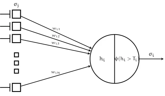
The concept I will first use to represent neurons is the McCulloch-Pitts for-malism. In this formalism neurons are logical units that function as “all or none” units, that either emit a spikes or do not fire. McCulloch and Pits first used binary threshold neurons to construct more complicated logical structures, such as AND, XOR, and NOT logical gates (McCulloch and Pitts, 1943). The McCulloch-Pitts neuron model captures enough detail to provide a rate based interpretation of brain activity, and they form the basis of artificial neural net-works such as the Hopfield model. Another important concept that this model cultivated early on in the computational neuroscience is the idea of neuronal inhibition playing a major role in steady state dynamics.
In the description given by McCulloch and Pitts (1943), see Figure 3, a neuron contains these components:
• A cell body, the soma, that consists of a post synaptic membrane poten-tial(PSP), and an activation function that maps input into a measure of activation.
σi
ψ(hi> Ti)
hi wi1
wi2
wi3 σj
[image:26.595.152.438.80.247.2]wiN
Figure 3:The major components of a McCulloch-Pitts artificial neuron. A neuroni re-ceives spikes from presynaptic neuronj, with strengthwij. Spikes are local-ized events in time,σi(t)is a boolean variable that represents that presence of a spike at timet.hiis the PSP at the soma, andψ(hi)is a function which detects spikes, withθirepresenting a firing threshold. Figure adapted from Amit (1989).
• A single output, the axon, that transmits spikes to other neurons in the network.
In a logical framework it is useful to model the presence of a spike on the axon as a boolean variableσi, but here we give a neuronia positive real valued firing
rateri. Each synaptic connection is associated with a synaptic weightwijwhich
signifies the amount to which the output firing rate of neuroniinfluences the
activation of neuronj. A neuron accepts a set of inputs, and it maps these to its
output, which represent the timing of output spikes. The process of computation takes place along the entire cell in the actual brain (Dayan and L. F. Abbott, 2001), with the spatial structure of the dendrites thought to play an increasing important role (London and Häusser, 2005), though we consider here only a single compartment of a cell’s soma. Formally, this computation requires that each neuron’s potential is associated with an activation function of its synaptic input, which we denote ashi. As an example, consider a neuron that simply
integrates synaptic, and input:
hi=X
j
rjwij, (1)
whererjis the firing rate of a neuronjwith a connection to neuroni, and
wijis a variable which describes the strength of the connection from neuronj
to neuroni.
The output firingrof a neuroniis a function of the input from the recurrent
connections (hi) and external input(ei). With the function
defined as the activation function. The activation function must be nonlinear (usually taken to be sinusoidal) to prevent positive feedback along the collaterals to cause the network to become unstable (E. T. Rolls, 2008).
1.2.1 Attractor network architecture
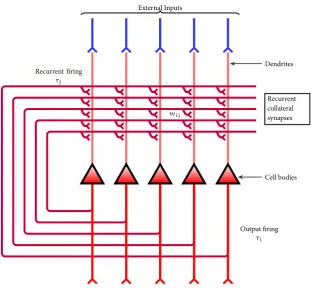
Neural networks can be classified based into different basic architectures that de-pends on the way the synaptic connections are arranged in the network. Neural networks can be thought of as a directed graph with N nodes, which represent neurons, and C edges, which represent the synaptic connections. Treves and Rolls have described two attributes that can be used to classify networks (E. T. Rolls and A. Treves, 1998). One attribute is the preferred direction of informa-tion flow, either recurrent or feedforward. The other attribute is the degree to which there is recurrent connectivity, or dilution, in the network. The recurrent connectivity of an attractor network is defined as the average number of connec-tions per neuron from neurons in the network divided by the total number of neurons in the network. The value of this parameter can therefore take values in the range of1/Nfor a fully diluted network to1for a fully connected network.
An attractor network has the output of each individual neuron feedback into the system alongrecurrent collaterals, see Figure 4. In order to model the propa-gation along the recurrent collaterals, we introduce the discrete time variablet.
At each time steptthe output of every neuron is used as input at timet+1. For
example, at timet=0, given an inputei, a network will produce firing in the
ensemble of neurons assigned toei, while the rest will remain silent. I refer to
the output firing of the neurons at a time by the rate vectorrt. In the case I
con-sider here, we taker0=ei. At each subsequent time step the network’s state will
be determined by strength of the recurrent collaterals as well as external input. I denote these recurrent collaterals as aN×Nweight matrixW, wherewijis
the weight between input unitiand output unitj, andNis the number of
neu-rons in the network. Neuronal firingr= {r1,r2,. . .,rN}produces recurrent
activationh={h1,h2,. . .,hN}along the synapses through the function
h=rW.
Population sparseness, α, is important parameter in neural networks that
measures the overall activation of the network. This parameter is used describe the encoding of memory patterns used to train the network. For instance, a low sparseness could be used to describe a pattern where only a few neurons are firing given a particular stimulus. Using data measured from populations of neurons in the real brain, Franco et al. (2007) found the population sparseness had an average value of0.77. Population sparseness is defined as:
α= (
PN
i yi
N)2
PN
i y2
i
N
whereyiis the mean firing rate of neuroni.
net-Recurrent collateral synapses External Inputs
Cell bodies Dendrites
Output firing ri
Recurrent firing rj
[image:28.595.152.464.81.371.2]wij
Figure 4:Connection diagram of a typical attractor network. External stimulus (in blue) is presented to each neuron at the cell body (red triangles), causing it to fire at rateri. The presence of external stimulus causes feedback into the network through the recurrent collaterls as described by the synaptic weight matrixW. The output firing will tend to settle into a steady pattern.
works with McCulloch-Pitts type neurons were often compared to spin glasses and other physical systems by Hopfield and others (Amit, 1989; Derrida, Gard-ner, and Zippelius, 1987; Gutfreund, 1990; Hopfield, 1982; Zippelius, 1993). It was this work that lead to rigorous analyses using both deterministic and stochas-tic dynamics. The techniques used in the analysis of the standard attractor net-work models assume that connections are reciprocal and symmetric in weight. If we adopt this set of assumptions we can use mean-field statistics to approx-imate free energy and mutual information in the network (E. T. Rolls and A. Treves, 1998). The approach used is related to Boltzmann’s theories of statistical mechanics, which seeks to describe the macroscopic features of a system by aver-aging over the microscopic interactions (Lebowitz, 1993). Mean field equations are a very useful tool in the study of oscillation in these network; for it frees us from concerning ourselves with microscopic details (Gerstner and Kistler, 2002).
The following application of a mean-field approach applied to the neuron model I have just described is adapted from Gerstner and Kistler (2002). In this example, we consider a population ofNMcCulloch-Pitts neurons that are time
a function of its synaptic input at any given time. Equation 1 is modified so that a neuron’s input is dependent on the other neurons’ activation in the previous timestep.
hi(t) =
N
X
j
rj(t−1)wij, (3)
In this example, the synaptic weights are taken to be excitatory and inhibitory in nature, and independent and identically distributed (i.i.d.) with probabilities given by
Pr[wij=1] = Cexc
N
Pr[wij= −1] =
Cinh
N (4)
WhereCexcandCinhrepresent the number of each type of synapse that the
neuron recieves.
A neuron will fire given that its post synaptic potential exceeds a firing thresh-old, these dynamics are given by
ri(t) =Θ[hi(t) −θi)],
whereθiis the firing threshold, andΘ[n]is the discrete Heavyside step func-tion.
The network is initialized with a random pattern of activity,
ri(t0)∈{0,1}, with probabilityri(t0) =1=a0,
wherea0represents the percentage of neurons that are active initially. We
can then calculate the firing in the subsequent time stepr(t1) by the
determin-istic dynamics of the system.
A neuron’s probability of being active in time stept = 1if it receives input
greater that its firing threshold. This is given by a sum over the probabilities of its synaptic inputs.
a1=a0
N
X
k=θi
k−θXi
l=0
Pr[L=l]Pr[K=k], (5)
whereKandLare random variables of the synaptic weights with distributions
given by Equation 4. In this equation, the outer sum is a sum over the chances of a neuron having a number of excitatory synapses greater than its threshold,
θi, and the inner sum is a sum over the chances that a neuron does not have
BecauseKandLare i.i.d. we may use a binomial distribution to calculate the
joint probabilities given in Equation 5.
a1=
N
X
k=θi
k−θXi
l=0
N
k
(a0CexcN−1)k(1−a0CexcN−1)N−k
N
l
(a0CinhN−1)l(1−a0CinhN−1)N−l.
(6)
ForCexc NandCinh N, the binomial distribution above is
approxi-mated by a Poisson distribution. Therefore, the probability than an input to a neuron will exceed its firing threshold is given by
a1=
N
X
k=θi
k−θXi
l=0
(ak+l0 CkexcClinh)
k!l! e
−a0(Cexc+Cexc). (7)
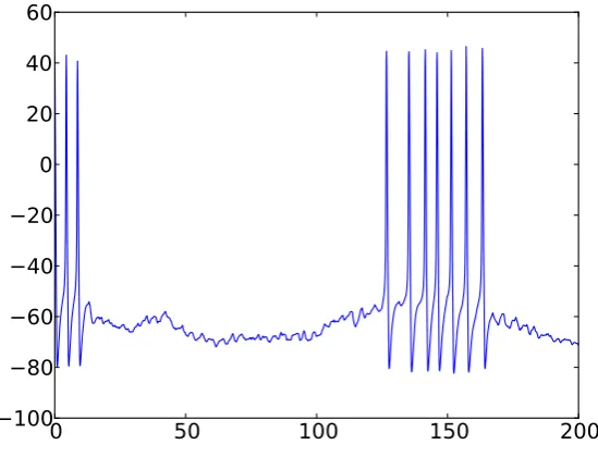
[image:30.595.183.409.379.597.2]This result can be generalized over all time steps through this recurrence re-lationship to find the steady state behavior of this network, for details consult Gerstner and Kistler (2002). A computer simulation of such a network is shown in Figure 5.
Figure 5:Firing of a recurrent McCulloch-Pitts neural network,Cexc=0.05,Cinh=
1.3
hopfield networks
A well known example of an attractor network is the Hopfield network (Hop-field, 2007), named after its inventor John Hopfield. In his famous 1982 paper, Hopfield described how an attractor network could function as a content ad-dressable memory system from the standpoint of dynamical systems theory. Hopfield networks were then used as a model network across many different fields, and was heavily analyzed with methods from statistical physics due to a direct mapping with the well understood Ising model (Amit, Gutfreund, and Sompolinsky, 1985).
I have so far assumed that each neuron in the network is updated synchronous at each time step. The Hopfield network lifts this assumption, and the update rule to each neuron may behave asynchronously, as one would assume in the real brain Amit (1989). When we randomly select the neurons to update at each time Hopfield network behave like a stochastic dynamical system (Rojas, 1996). The neurons first described in Hopfield nets were binary threshold units, i.e. neurons can either take on a state 1 or 0. State 1 corresponds to the neuron firing at its maximum rate, denotedri =1, and state 0 corresponds to the
neu-ron not firing. A neuneu-roniin the network has the threshold binary activation
function:
ri=
1 ifPjwijrj> θi
0 otherwise (8)
withθi=0being the threshold for neuroni.
I have said that attractor networks function to encode patterns of neural ac-tivations. In order to do this the network must undergo learning. The patterns we wish to store in an attractor network are represented by a vector of rates of lengthN, denoted hereep = {eip,. . .,epN}. Our goal is after presentation of
a fragment of an encoded pattern along the network’s external inputs to have the firing of the network eventually reaching some stable firing pattern. We can then compare the firing of the network in this final state with the learned patterns. In the Hopfield model patterns are learned by the network through synaptic modification in accordance with Hebb’s rule,
wij= N1 PP
p
epiepj wherei6=j
wij=0, wherei=j,
(9)
wherePis the number of patterns we wish to store. All patterns can be stored
in one iteration of presenting each pattern to the network, calculating the acti-vation, and updating the synaptic weights using Equation 9; this is a process called one-shot Hebbian learning. Proper application of this algorithm causes a network to learn the broad statistical structure of the inputs (O’Reilly, 1998), making it suited to preform well with a set of input vectors with uniformly dis-tributed values.
postsynap-tic neurons which share the weight. Hebb’s rule is commonly interpreted to say that a change in the synaptic weight between two connected neurons is a function of the weighted product of their firing rates.
∆wij=krirj, (10)
and Equation 9 extends this rule across a vector of patterns.
The network performs recall operations through a dynamical update of state. There are procedures for both updating a Hopfield network sequentially (asyn-chronously) or parallel (syn(asyn-chronously). In the sequential case the update of the network is done by first choosing a neuroniat random; and then ifPjriwij+
ei > θithen setri=1, otherwise setri=0.
One of Hopfield’s major breakthroughs was the definition of an energy land-scape, with basins of attraction, of the different possible states of the memory system. In recall, partial cues are presented to the network by setting each neu-ron’s external input. This starts the network firing in a state which lies inside a basin of attraction. The system will then settle down into a state that corre-sponds to a stored pattern through the updating procedure. A Hopfield network is designed to store and retrieve a number of patters up to a certain critical value, after which the network will catastrophically fail (Kanter and Sompolinsky, 1987; E. T. Rolls and A. Treves, 1998). This critical value,αc≡p/N, is dependent on
the type of pattern stored, the connectivity of the network, and the sparseness. Some authors have found that for Hopfield networksαc≈0.14(Crisanti, Amit,
and Gutfreund, 1986). Using other methods, multiple other authors have ana-lyzed the standard Hopfield model, and they have found thatαc(with all stored
memories being recallable) asymptotes atN/(4log(N))memories (Feng and Tirozzi, 1997; McEliece et al., 1987).
The spareness of the memory patterns is a major factor determining the stor-age capacity of the network. Training the network with patterns of low spareness will increase the amount of patterns that can be stored (E. T. Rolls and A. Treves, 1998). Intuitively, this increased storage capacity can be interpreted as a result of having less overlap of the same neurons firing in two different patterns be-cause there are less neurons firing over all. Treves and Rolls 1998 described the storage capacityαcin terms of the parameters of connectivity and sparseness:
pmax∼
C
aln(a1)k (11)
wherekis a constant around0.2−0.3.
These basins of attraction, which are local minima of an energy function, cor-respond to steady state values of the system. In these steady states, the firing of the neurons is the same as the stored memory patterns. The energy landscape of a Hopfield network is defined by the function
E= −1/2
N
X
i N
X
j
wijrirj−
N
X
i
The tendency of the Hopfield network to settle and stay in one particular basin, from the set of possible basins defined by the energy landscape, means that it is classified as a point attractor in the dynamical systems taxonomy of at-tractor networks. This taxonomy includes stable point, line, and ring atat-tractors; and unstable cyclic, and chaotic attractors (Eliasmith, 2007).
The energy landscape shows how pattern completion and the memory re-call can occur under different conditions. With this formulation Hopfield shed tremendous light on the question of how many memories an attractor network can store.
Up to this point I have only considered binary representations for the neu-rons. Neurons in the brain fire with continuously variability. Continuous firing rates were analyzed by Hopfield (1984). He replaced the binary neurons in his original network which neurons which continuously increased in activity when exposed to greater input. The firing rate of these neurons were bound on both sides by a minimum, usually0, and maximum firing rate. Hopfield also
mod-eled a lag in the synaptic current reaching the soma after the behavior of real neurons.
In graded pattern representations, neurons can fire at many different discrete rates. For example, one step up from a binary representation would be a ternary representation. In a ternary representation the neuron can either not fire, fire at a low rate, or fire at a highly rate. Using a high graded pattern representation of the memories will not change the storage capacity of the network from using a lower representation. Theoretical analysis and simulation results show that such a network is able to store a similar number of patterns using graded patterns of composed of10and50graded rates (E. T. Rolls et al., 1997a; A. Treves and E. T.
Rolls, 1991). The performance of the network will vary with the type of pattern used for training and recall. Simulation results show that recall performance of an attractor network trained with patterns of neurons that can fire at10different
rates is markedly worse than the same network trained with binary patterns (E. T. Rolls et al., 1997b).
2
S P I K I N G N E U R A L N E T W O R K
M O D E L S
B
iologically accurate mathematical descriptions of neurons first appeared in earnest with the seminal work of Hodgkin and Huxley. Hodgkin and Huxley mathematically modeled the squid giant axon using dynamics that accounted for the concentration of ions inside and outside the neuron mem-brane. The ions flow in and out of the membrane through dynamics dependent on biologically plausible gating variables. For the time, the model was extraor-dinarily detailed with respect to the functioning of ion channels, and60yearsafter their1952paper the Hodgkin-Huxley (HH) neuron model is still in use
(D. Noble, Garny, and P. J. Noble, 2012). The Hodgkin-Huxley model is very good at capturing the type of behavior measured from actual neurons, yet it has a relatively high computational demand, compared to other non-spatial spiking neuron models. Often, in the past, the model has only been effective in smaller network simulations (Izhikevich, 2004). More recently, advanced library inte-gration techniques have been developed, that can simulate HH neural networks with a computational efficiency comparable to using a simpler spiking neuron model, without sacrificing the rich dynamics of a HH network (Sun et al., 2009). I will first describe the need for more detailed models than the artificial neu-ron described in the preceding chapter. Neuneu-rons in the brain have a difference in electrical charge between the extracellular region and the intracellular re-gion. This is known as a neuron’smembrane potential. This is due to a carefully managed balance of electrically charged ions across the cell’s lipid bilayer. An equation that can describe the equilibrium or resting potential of neurons was first devised by Walther Nernst (Stock and Orna, 1989). Later, Goldman (1943) mathematically described how ionic current will behave when the current is not equal to the resting potential. Crucially these dynamics must be understood to model neurons that capture realistic spiking behavior using detailed ion dynam-ics, such as Hodgkin-Huxley type neurons. However, neuroscientist have been interested in the different levels of abstraction at which one can model neurons and still approximate more realistic behavior (Herz et al., 2006). I consider here models that exist at the level of abstract ion dynamics, but detailed in the behav-ior of the membrane potential. This makes them more detailed than the type of dynamics used by the artificial neuron models described in chapter 1. This level of detail is well suited for studying very large populations of neurons, in excess of
100,000, where the individual timings of spikes play a role. Neurons with
spik-ing dynamics are also used to study spike timspik-ing dependent plasticity (STDP) (Bi and Poo, 1998; Caporale and Dan, 2008), effects of spike related stochasticity (Amit and Brunel, 1997b), and neural coding (Gütig and Sompolinsky, 2006).
neu-ron using a standard method such the Euler or Runge-Kutta method. This ap-proach is easy to implement, but suffers from errors introduced by numerical integration, and is computationally expensive in that every neuron in a network must be updated at every timestep. To correct for the error a small integration timestep must be chosen, resulting in a speed/accuracy trade off. Another more sophisticated approach is the event-driven method. Using this approach the network is updated in the following three steps: 1) analytically determine the time of the soonest spike in the network, 2) advances the network to that time value and analytically determines each neurons new potential at the new time step, 3) propagate the PSP from the neuron that just fired, and repeat. This ap-proach results in faster simulations (Cessac and Viéville, 2008), and it depends on synaptic interaction terms being analytically tractable; however, approxima-tions for conductance based synapses have been proposed (Rudolph and Des-texhe, 2006). Stewart and Bair (2009) developed a promising new method for simulation based on the Parker-Sochacki method and presented results of in-creased speed/accuracy payoff. Modern graphics processing units, one can sim-ulate a network of55,000spiking neurons at real time speeds (Nowotny, 2011),
cluster based simulations of neuron networks have been preformed with almost half a billion synapses (Izhikevich and Edelman, 2008).
0 50 100 150 200
[image:35.595.163.438.350.560.2]−100 −80 −60 −40 −20 0 20 40 60
Figure 6:Simulation of Hodgkin-Huxley type neuron using exponential Euler integra-tion. Single neuron recording taken from a4000neuron network of
excita-tory and inhibiexcita-tory neurons. Parameters taken from (Brette, Rudolph, et al., 2007).
(L. F. Abbott, 1999; Brunel and Rossum, 2007). The simple dynamics used by this model is adequate only at describing the subthreshold behavior of a neu-ron’s membrane potential, because the action potential is not explicitly mod-eled. Other extensions to the IF model exist, including the exponential IF model (Fourcaud-Trocmé et al., 2003), quadratic IF model (Brunel and Latham, 2003), adaptive exponential IF model (Brette and Gerstner, 2005), and resonate and fire model (Izhikevich, 2001). Given these other options, Izhikevich (2004) states that the leaky IF model is a poor choice when it comes to biological real-ism, because it lacks key features such “phasic spiking, bursting of any kind, re-bound responses, threshold variability, bistability of attractors, or autonomous chaotic dynamics.”
IF dynamics (Burkitt, 2006; Knight, 2000) describe the membrane potential of neurons. We can choose biologically realistic constants to obtain firing rates that are comparable to experimental measurements of actual neural activity. IF neurons integrate synaptic current into a membrane potential, and then fire when the membrane potential reaches a voltage threshold. The equation that governs the membrane potential of a neuronViis given by
CmdVi(t)
dt = −gm(Vi(t) −VL) −Isyn(t), (13)
whereCmis the membrane capacitance,gmis the leak conductance,VLis the
leak reversal potential, andIsynis the total synaptic input. A spike is produced
by a neuron when its membrane potential exceeds a thresholdVthr= −50mV
and its membrane potential is reset to a valueVreset = −55mV. Neurons are
held atVresetfor a refractory periodτrpimmediately following a spike.
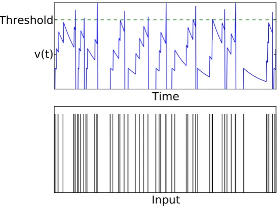
Neurons in the brain do not receive constant input current. One of the early elaborations of the non-leaky IF model to account for stochastic input was given by G. L. Gerstein and Mandelbrot (1964), later extended by Stein (1965) to the leaky version of the model, and reviewed by Wilbur and Rinzel (1982). Here, the variation of a neuron’s membrane potential away from equilibrium is governed by the stochastic set of presynaptic spikes that the neuron receives. In such a regime, we let the membrane receive synaptic input that be described by a Poisson process. Each event in the Poisson process corresponds to a presynaptic spike arriving at the neuron. On the arrival of a event the neuron receives a depolarizing “kick” to its membrane potential, as shown in Figure 7.
The stochastic input to a neuron is usually modeled as a set of delta functions that represent the shot noise of presynaptic input. IF neurons are one compart-ment models with presynaptic spiking having a direct effect on the membrane through a postsynaptic activation function. Burkitt (2006) outlines common synaptic types are used to represented the activation functioncurrent synapses orconductance based synapses. Current synapses provide a linear post synaptic potential (PSP) that does not depend on the membrane potential of the post synaptic neuron, while conductance based synapses provide a nonlinear PSP that depends on the difference between the membrane potential and its reversal potential. Typical models link a perceptual decision to the activity of a subpop-ulation of neurons (Braun and Mattia, 2010).
Time
v(t)
Threshold
[image:37.595.158.431.103.307.2]Input
Figure 7:Effect of stochastic spiking input on a neuron’s membrane potential. Top: A neuron’s membrane potential is increased towards the firing threshold for every presynaptic spike it receives (bottom).
extended to population dynamics. The approximations has been described by Gerstner and Kistler (2002) and Burkitt and Clark (2000). In this model one ignores the firing threshold and instead considers the unrestricted path of the membrane potential. This notion can be extended to work out the firing rate of a neurons by calculating the moments of the input. Amit and Brunel (1997b) used Gaussian approximation to obtain steady state dynamics of spontaneous (low firing rate) neuron activity, which has paved the way for the majority of the work conducted in this thesis.
2.1
an integrate-and-fire attractor
neuronal network model of
decision-making: methods used throughout
the thesis
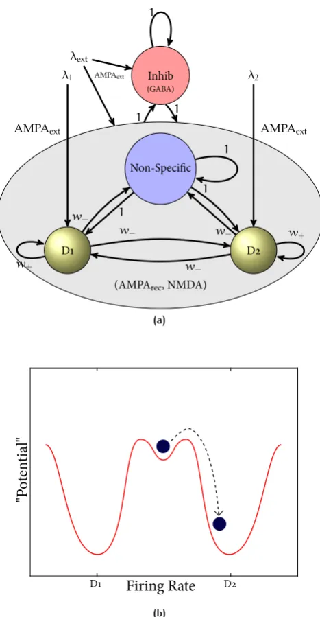
In this section I will present the methods used throughout the rest of the thesis. The probabilistic decision-making network I use throughout this thesis is in the mold of a spiking neuronal network model with a mean-field equivalent (X.-J. Wang, 2002). I set the network to operate with parameters determined by the mean-field analysis that ensure that the spontaneous firing rate state is stable even when the decision-cues are applied, so that it is only the noise that provokes a transition to a high firing rate attractor state, allowing the effects of the noise to be clearly measured (Deco and E. T. Rolls, 2006; E. T. Rolls and Deco, 2010).
What follows in this section is the description of the model. Its application to decision-making is first presented in chapter 3; however, I will mention a few aspects of biological function that this model does capture at the end of the section.
The fully connected network consists of separate populations of excitatory and inhibitory neurons as shown in Figure 8. Two sub-populations of the exci-tatory neurons are referred to as decision pools, ‘D1’ and ‘D2’. The decision pools each encode a decision to one of the stimuli, and receive as decision-related in-putsλ1andλ2. The remaining excitatory neurons are called the ‘non-Specific’
neurons, and do not respond to the decision-making stimuli used, but do allow a given sparseness of the representation of the decision-attractors to be achieved. (These neurons might in the brain respond to different stimuli, decisions, or memories.) A description of the network follows.
The network consists ofNneurons, withNE = 0.8Nexcitatory neurons,
andNI=0.2Ninhibitory neurons. The two decision pools are equal size
sub-populations with the proportion of the excitatory neurons in a decision pool, or the sparseness of the representation with binary encoding,f=0.1. The neuron
pools are non-overlapping, meaning that the neurons in each pool belong to one pool only.
We structure the network by establishing the strength of interactions between pools to take values that could occur through a process of associative long-term potentiation (LTP) and long-term depression (LTD). Neurons that respond to the same stimulus, or in other words ones that are in the same decision pool, will have stronger connections. The connection strength between neurons will be weaker if they respond to different stimuli. The synaptic weights are set ef-fectively by the pre-synaptic and post-synaptic firing rate reflecting associative connectivity (E. T. Rolls, 2008). In the representation case neurons in the same decision pool are connected to each other with a strong average weightw+,
and are connected to neurons in the other excitatory pools with a weak aver-age weightw−. All other synaptic weights are set to unity. Using a mean-field
analysis which applies to the firing rate distribution case (Deco and E. T. Rolls, 2006), we chosew+to be near2.1, andw−to be near0.877to achieve a