Implied distributions in multiple change point problems

University of Warwick institutional repository: http://go.warwick.ac.uk/wrap

This paper is made available online in accordance with publisher policies. Please scroll down to view the document itself. Please refer to the repository record for this item and our policy information available from the repository home page for further information.

To see the final version of this paper please visit the publisher’s website. Access to the published version may require a subscription.

Author(s): J. A. D. Aston, J. Y. Peng and D. E. K. Martin

Article Title: Implied distributions in multiple change point problems Year of publication: 2011

Link to published article:

http://dx.doi.org/10.1007/s11222-011-9268-6

J. A. D. ASTON1_{, J. Y. PENG}2_{AND D. E. K. MARTIN}3

1_{CENTRE FOR RESEARCH IN STATISTICAL METHODOLOGY, UNIVERSITY OF WARWICK} 2_{INSTITUTE OF INFORMATION SCIENCE, ACADEMIA SINICA}

3_{DEPT. OF STATISTICS, NORTH CAROLINA STATE UNIVERSITY}

ABSTRACT. A method for efficiently calculating exact marginal, conditional and joint distri-butions for change points defined by general finite state Hidden Markov Models is proposed. The distributions are not subject to any approximation or sampling error once parameters of the model have been estimated. It is shown that, in contrast to sampling methods, very little com-putation is needed. The method provides probabilities associated with change points within an interval, as well as at specific points.

Date: June 20, 2011.

Key words and phrases. Finite Markov Chain Imbedding; Hidden Markov Models; Change Point Probability; Run Length Distributions; Generalised Change Points; Waiting Time Distributions.

1. INTRODUCTION

This paper investigates some exact change point distributions when fitting general finite state

Hidden Markov models (HMMs), including Markov switching models. Change point

prob-lems are important in various applications, including economics (Hamilton 1989; Chib 1998;

Sims and Zha 2006) and genetics (Durbin, Eddy, Krogh, and Mitchison 1998; Eddy 2004;

Fearnhead and Liu 2007). In many instances change point problems are framed as product

partition models (Barry and Hartigan 1992; Barry and Hartigan 1993) or HMMs (Chib 1998;

Fr¨uhwirth-Schnatter 2006; Fearnhead and Liu 2007), however, to date, the characterisation

of the change point distributions implied by these models has been mostly performed using

sampling methods (Albert and Chib 1993; Capp´e, Moulines, and Ryd´en 2005), exact

poste-rior sampling (Fearnhead 2006; Fearnhead and Liu 2007), or the distributions are ignored and

deterministic algorithms such as the Viterbi algorithm (Viterbi 1967) or posterior (local)

de-coding (Juang and Rabiner 1991) are used to determine the implied change points. Methods

have also been suggested for using a forward-backward like algorithm to get efficient samples

based on the Viterbi sequence (Gu´edon 2007), resulting in posterior distributions for change

points (Gu´edon 2008). In contrast to these previous methods, the distributions in this paper are

exact (in the applied probability sense) in that, conditioned on the model and parameters, they

completely characterise the probability distribution function without requiring any asymptotic

or other approximation or being subject to any sampling error. It will be shown that these

dis-tributions can be calculated in many cases using a small number of calculations compared to

those needed to yield an approximate distribution through sampling.

The method can be used to determine probabilities of whether a change in regime has

oc-curred at any particular time point. This will be evaluated through a concept called the change

point probability (CPP), which is a function of the marginal probabilities of particular time

or-dered change points occurring at certain times. The marginal probabilities are determined after

finding the joint and conditional distributions of multiple change points. Using the marginal

distributions allows a probabilistic quantification of the relationship between changes in the

A model might be deemed to capture the influence of an event causing a change in the

data when the probability distribution of a change point around the time point of the event is

peaked. In contrast, a model for which the probability of a change in regime is more uniform

indicates that the regime specified by the model is not particularly affected at that or any other

particular point. To illustrate this point, US Gross National Product (GNP) regime switches will

be examined in relation to the CPP of recession starts and ends as determined by the National

Bureau of Economic Research (NBER). The NBER can be seen as providing external estimates

of change points based on overall economic data. Comparing change points determined by the

NBER and those determined by maximisation of local posterior state probabilities (Hamilton

1989) leads to the surprising result that regime switches determined from the latter method may

not be a useful metric. In contrast, the CPP gives the exact probability of a change occurring at

any time point or interval, given the model.

HMMs are widely used in statistics and engineering; see MacDonald and Zucchini (1997)

and Capp´e, Moulines, and Ryd´en (2005) for good overviews on the current state of the art both

in theory and applications of them. To locate change points (or equivalently to perform data

segmentation) HMMs are generally trained on data and then applied to test data (Rabiner 1989;

Durbin et al. 1998). The methodology of this paper is appealing in that it allows complete

quantification of uncertainty in test data analysis. This methodology is generic in that it

de-pends only on the Markovian nature of regime switches and the ability to generate posterior

probabilities, and not upon the structure of any particular HMM model.

The structure of the paper is as follows. Section 2 contains the methods to find change

point distributions from data via HMMs and the use of waiting time distributions. Also in that

section, the joint and marginal distributions of a set of change points are derived and the concept

of CPP is defined. Section 3 contains applications of the methodology to Chib’s (1998) change

point model and the GNP data given by Hamilton (1989). Section 4 contains a few concluding

In the supplementary material, a basic smoothing algorithm for Markov switching models

will be given, completing an algorithm given by Kim (1994) so that the smoother contains all

needed terms.

2. WAITING TIME DISTRIBUTIONS AND CHANGE POINTS

The methods that will be presented here can be applied to general finite state Hidden Markov

Models (including Markov switching models) with the form:

yt ∼ f(St−r:t, y1:t−1), t= 1, . . . , n

P[St0|S−r_+1:t0₋₁] = P[S_t0|S_t0₋₁], t0 =−r+ 2, . . . . (2.1)

The datayt from time 1 to time n is distributed conditional on previous data and r previous

switching states St−r, . . . , St−1 in addition to the current stateSt (as well as model

parame-ters, the values of which are implicitly assumed to be fixed). Here, yt1:t2 = yt1, . . . , yt2 with

St1:t2 defined analogously. For simplicity, the switching states{St}are assumed to be a

first-order Markov chain with finite state spaceS, but extension to higher-order Markov structures

is straightforward. A given initial distribution π for S−r+1:0 is also assumed. With suitable

modification, the above model may also include exogenous variables. No assumption on the

distribution of the data is made other than that the posterior probabilities of the states

(proba-bilities conditional on the data) must exist.

Definition A run of lengthk in states is defined to be the consecutive occurrence ofk states that are all equal tos, i.e.St−k+1 =s, . . . , St=s(c.f. Feller (1968), Balakrishnan and Koutras

(2002)).

Herekwill always represent the minimum length of the regime to be considered or equivalently

the length of run to be found. Now form ≥1, letWs(k, m)denote the waiting time of themth

run of length at leastk in states, and letW(k, m)denote the waiting time for themth run of

length at leastkof any states∈ S. Note thatW(k, m)is invariant under any state re-labelling,

Consider, for example, the case of growing (s = 1) and falling GNP (s = 0). W0(k,1)is

then the first time that a period of falling (

=k

z }| {

0. . .0) GNP has occurred in{St}whereasW(k,1)

is the first time either a period of falling GNP or growing (

=k

z }| {

1. . .1) GNP occurs. By changing

the value ofk, shorter or longer length periods can be investigated.

A change point at timetis typically defined to be any time at whichSt−1 6=St, the beginning

of a run of length at least one. A special case is given in Chib (1998), where the states are

re-quired to change in ascending order. However, a more general definition is allowed here, where

a change point is defined to have occurred when a change persists at leastktime periods,k ≥1.

A classic example of when the generalised definition is needed is the common definition of a

recession, where two quarters of decline are required (k = 2) before a recession is deemed to

be in progress. Letτ_i(k),i= 1, . . . , mbe the time of theith change point under this generalised

definition. Then

P[τ_i(k) =t] =P[W(k, i) = t+k−1]. (2.2)

Equation (2.2) follows because theith run of length at leastkoccurs at timet+k−1if and only

if the switch into that regime has occurredk−1time points earlier. Whenk = 1, it is assumed

in this work that a change point has occurred att= 1, i.e.P[W(1,1) = 1] =P[τ₁(1) = 1] = 1,

and hence the ith change point using the common definition will be equivalent to (i+ 1)st

change point τ_i(1)₊₁ as defined here. Since the Markov chain is assumed to continue even after

the observed data, a regime or run of length at leastk can appear even after timenand hence

P[τ_i(₊₁k) > n]≥P[τ_i(k)> n]≥0.

Other distributions can be calculated from the waiting time distribution. For example, the

distribution of the maximal length of a regime ins,Rs(t), up to timetis given by

P[Rs(t) = k] = P[Rs(t)≥k]−P[Rs(t)≥k+ 1]

= P[Ws(k,1)≤t]−P[Ws(k+ 1,1)≤t]. (2.3)

Analogously, the probability that the maximal length of any regime isk,P[R(t) = k], can be

defined in terms ofP[W(k,1) ≤t]. In addition, the number of regime changes into state sof

2.1. Methods to Calculate Waiting Time Distributions for the First Change Point. Finite Markov chain imbedding will be used to compute distributions associated with the regime

peri-ods. These methods have been used previously for Markovian problems (Fu and Koutras 1994)

and HMMs with discrete observations (Aston and Martin 2007) where it was assumed that

there was no dependence between observations except through the underlying Markov chain.

The method presented here involves imbedding the {St} sequence into a new Markov chain

{Zt}with a larger state space. Though{St}forms a homogeneous Markov chain, conditioning

on the data inducesrth order inhomogeneous dependence, i.e. the posterior transition

proba-bilitiesP[St|St−r:t−1, y1:n]are transition probabilities of an inhomogeneousr-th order Markov

process (Capp´e, Moulines, and Ryd´en (2005) and supplementary material).

The state space of {Zt} (which is denoted by Zs or Z depending on whether runs of a

particular states or a run of any state is of interest) will consist of vector states of the form

((st−r+1, . . . , st), j). The component (st−r+1, . . . , st) ∈ Sr, necessary due to the rth-order

dependence of states conditional on the datay1:n, gives the values of the last r states at time

t, t = 0, . . . , n. The component j, j = 0,1, . . . , k, gives the length of the current run of a

particular state s (j = max1≤φ≤k : St = s, St−1 = s, . . . , St−φ+1 = s if St = s, j = 0

otherwise), or of the current value ofStif general runs are of interest. Ifk > r,

Zs = r−1 [ j=0    [

st−r+1:t:sl=s,l=t−j+1,...,t;sl∈S,l=t−r+1,...,t−j

(st−r+1:t, j)

   ∪ k [

j=r

((s, . . . , s), j) !

,

(2.4)

and ifk ≤r,

Zs = k [ j=0    [

st−r+1:t:sl=s,l=t−j+1,...,t;sl∈S,l=t−r+1,...,t−j

(st−r+1:t, j)

  

, (2.5)

where any stringssa:bwitha > bor anysb withb < t−r+ 1are ignored. (Notice that in (2.4)

and (2.5), some states are needed only for the initialisation stage whent < r).

Whenj = k, a run of lengthk or longer has occurred. The set Aof states with j = k are

one. The state spaceZ for calculatingP[W(k,1)≤t]is then

Z = [

s∈S

Zs. (2.6)

Let z∗ represent the size of either Zs or Z as appropriate. As the components of states

of {Zt} are functions of states {St}, the |S| non-zero row entries in the z∗ ×z∗ transition

probability matrixMt for transitions from transient states of{Zt}are completely determined

by the posterior transition probabilitiesP[St|St−r:t−1, y1:n]. Specifically,

P[Zt = ((st−r+1, . . . , st), j)|Zt−1 = ((st−r, . . . , st−1), l), y1:n]

=P[St=st|St−1 =st−1, . . . , St−r=st−r, y1:n] (2.7)

for appropriate values ofj which are determined in the following manner: for transient states

of Zs, j = l+ 1 when st = s, and j = 0 if st 6= s. For transient states of Z, j = l + 1

whenst=st−1, andj = 1ifst 6=st−1. In the supplementary material, a completion of Kim’s

algorithm is given for the purpose of calculating the posterior transition probabilities of (2.7).

The initial probability distribution forZ0is contained in the1×z∗row vectorψ0, which has

non-zero probabilities

ψ0((s−r+1, . . . , s0),0) =P[Z0 = ((s−r+1, . . . , s0),0)] =π(s−r+1, . . . , s0). (2.8)

From the well-known Chapman-Kolmogorov equations for Markov chains (Feller 1968), it

follows that the 1×z∗ probability vectorψt of Zt lying in its various states at timet ≥ 1is

given by

ψt=ψ0

t

Y

l=1

Ml. (2.9)

The waiting time distributionP[Ws(k,1)≤t]can then be calculated as

P[Ws(k,1)≤t] =P[Zt∈A] =ψtU(A), (2.10)

with the analogous result holding forP[W(k,1) ≤ t], where U(Ω)is az∗×1column vector

since the Markov chain{Zt}is in an absorbing state if and only if a run of length at leastkhas

occurred. Combining (2.9) and (2.10), fort≥k,

P[Ws(k,1) =t] =P[Ws(k,1)≤t]−P[Ws(k,1)≤t−1] =ψ0

t−1 Y

l=1

Ml

!

(Mt−I)U(A),

(2.11)

whereI is az∗×z∗identity matrix.

2.2. Methods to Calculate Waiting Time Distributions for Multiple Change Points. In this subsection, a method is given to calculate joint probabilities associated with change points

through augmenting the state spaces Zs andZ. Manipulations of the joint probabilities will

lead to an algorithm for computing marginal change point distributions. The algorithm obviates

the need to repeat states for each of thei= 1, . . . , mchange point occurrences.

2.2.1. Setup of Markov Chain for Distributions Associated with Multiple Change Points. A set

of states C, called continuation states, is added to Zs and Z, and the respective sizes z∗ are

incremented by the number of continuation states. The role of the continuation states is that

once the ith run of length at leastk has occurred, a new Markov chain {Z_t(i+1)} is started to

determine probabilities associated with the next occurrence of a run of the desired length. The

continuation states serve to initialise the new chain{Z_t(i+1)}, and indicate that runi is still in

progress and needs to end before the(i+ 1)st run can begin.

The continuation states((st−r+1, . . . , st),−1)∈Ccorrespond to absorbing states((st−r+1, . . . , st), k)

∈ A, with -1 indicating that a run continues and must end for the next run to begin. The (less

than full rank)z∗×z∗ matrixΥdefined by

Υ (z1, z2) =     

1 ifz1 ∈Aandz2 ∈Cis the corresponding continuation state

0 otherwise

(2.12)

maps probabilities of being in the states ofA into probabilities for being in the corresponding

states ofC.

The transition probability matrices Mt are revised to account for the continuation states.

Continuation states may only be entered from other continuation states. The generic

conditional on the data are of the form

P[Zt= ((st−r+1, . . . , st), j)|Zt−1 = ((st−r, . . . , st−1),−1), y1:n]

=P[St =st|St−r =st−r, . . . , St−1 =st−1, y1:n], (2.13)

where the appropriate values ofj for (2.13) are determined by:

(1) Ifst=st−1,j =−1for bothZsandZ;

(2) Ifst6=st−1, thenj = 0forZs, andj = 1forZ,

with the lastj = 1following as runs in any state are of interest. The transition probabilities for

the rest of the states in eitherZsorZ are unchanged.

2.2.2. Computation of Joint, Conditional and Marginal Distributions. The joint distribution of

the firstmchange points can be factorised as

P[τ_m(k)=tm, . . . , τ

(k)

1 =t1] =P[τ (k) 1 =t1]

m

Y

i=2

P[τ_i(k) =ti|τ

(k)

i−1 =ti−1, . . . , τ (k) 1 =t1],

(2.14)

which will equal zero if the distance between anyti andti−1 is less thank. If

Qb

l=aMl

=I

forb < a, then by (2.11),

P[τ₁(k) =t1] =P[W(k,1) = t1+k−1] = ψ0

t1+k−2

Y

l=1

Ml

!

(Mt1+k−1−I)U(A). (2.15)

To calculateP[τ_i(k) =ti|τ

(k)

i−1 =ti−1, . . . , τ (k)

1 =t1], define

ξ_t(1)_1+k−1 =ψ0

t1+k−2

Y

l=1

Ml

!

(Mt1+k−1−I). (2.16)

and fori= 2, . . . , m

ξ_t(i)

i+k−1 =

ξ_t(i−1)

i−1+k−1Υ

ξ_t(i−1)

i−1+k−1U(A)

! 

ti+k−2

Y

l=ti−1+k

Ml



(Mti+k−1 −I). (2.17)

By (2.15) and (2.16), P[τ₁(k) = t1] = ξ (1)

t1+k−1U(A). The vectors

_ξ(i−1) ti−1+k−1Υ

ξ_ti(i−1)

−1+k−1U(A)

serve as

the initial distribution for the excursion of the Markov chain{Z_t(i)}beginning in a continuation

state at timeti−1+k−1, analogous toψ0for the first chain at time zero, and

Thus, fori= 2, . . . , m, the joint probability

P[τ_i(k)=ti, . . . , τ1(k)=t1]

= P[W(k, i) =ti+k−1, . . . , W(k,1) =t1+k−1]

= i

Y

q=1 ξ_t(q)

q+k−1U(A)

= ψ0

i−1 Y q=1    

tq+k−2

Y

l=tq−1+k

Ml



(M_tq+k−1−I)Υ 

 



ti+k−2

Y

l=ti−1+k

Ml



(M_ti+k−1−I)U(A), (2.19)

wheret0 ≡1−kfor convenience.

Marginal distributions for change point τ_i(k), or equivalently the marginal waiting time

dis-tribution for theith run occurrence,i= 2, . . . , m, can then be written as

P[τ_i(k)=ti] = P[W(k, i) =ti+k−1]

= X

1≤t1<ti

. . . X

ti−2<ti−1<ti

P[W(k, i) =ti+k−1, . . . , W(k,1) =t1+k−1]

= X

1≤t1<ti

. . . X

ti−2<ti−1<ti

i

Y

j=1 ξ_t(j)

j+k−1U(A)

=

 

 X

ti−2<ti−1<ti

. . .  

 X

t1<t2<ti

 

 X

1≤t1<ti

ξ(1)_t

1+k−1U(A)

 

 ξ(2)_t

2+k−1U(A)

   . . .    ξ_t(i)

i+k−1U(A)

(2.20)

with the marginal distributionP[τ₁(k) =t1]given by (2.15).

Equation (2.20) suggests the use of some form of sum-product algorithm (for a definition of

the sum-product algorithm see Kschischang, Frey, and Loeliger (2001)) for its calculation. Let

ψ_t(i) be row vectors carrying probabilities for the Markov chain Z_t(i), i.e. the joint probability

that the (i−1)st run has occurred by time t, and that the chain lies in any one of its states at

timet(so thatψ_t(1) =ψt). The marginal distributions are then

P[τ_i(k)=ti] =P[W(k, i) =ti+k−1] = (ψ

(i)

ti+k−1−ψ

(i)

ti+k−2)U(A), (2.21)

the probability of being absorbed at timeti+k−1, and a similar formula holds forWs(k, i).

Two operations need to be carried out to updateψ(_t−i)₁ toψ_t(i): (1) Due to the Markovian nature

probabilities for the (i−1)st run occurrence must be incremented since they give initial

prob-abilities when waiting for the occurrence of theith run. These operations may be carried out

simultaneously fori= 1, . . . , mby replacing (2.9) with the following matrix computations.

LetΨt,t = 0, . . . , nbem×z∗matrices withith rowψ

(i)

t . The initial matrixΨ0 then has as

its first rowψ0, with the remaining rows being composed of zeroes since the probability is zero

that a run has occurred at timet= 0. The algorithm fort = 1, . . . , nis

Ψt = Ψt−1Mt, (2.22)

ψ_t(i) ← ψ_t(i)+ψ_t−(i−₁1)(Mt−I)Υ, i= 2, . . . m, (2.23)

where (2.22) is related to computing the matrix product

Qti+k−2

j=ti−1+kMj

of (2.19) while (2.23)

is related to computing(Mti−1+k−1−I)Υ,i= 2, . . . m.

Even though the algorithm is non-linear, it can be carried out in linear time w.r.t. t, as the

non-linear update step (2.23) is just a simple alteration to entries in the matrix Ψt, requiring

only linear time computations.

Using the calculations given above, the distribution of the number of regime changesP[Ns(k) =

i]into a particular state is given by

P[Ns(k) =i] =P[Ws(k, i)≤n]−P[Ws(k, i+ 1)≤n], i= 0, . . . , ζ+b

n−(k+ 1)ζ

k c,

(2.24)

where bxc indicates the integer part of x and ζ = b n

k+1c. In practice, the value at which

P[Ws(k, i) ≤ n] becomes negligible will be i ζ +b

n−(k+1)ζ

k c. Analogous results hold

for probabilities P[N(k) = i] associated with the number of change points in the data, by

consideringP[W(k, i)≤n]fori= 0, . . . ,bn/kc.

By using the setup above it is also possible to determine distributions associated with the end

of a regime (the first time point after a run of length at leastk has occurred where the process

is no longer in the run state). Let W_se(k, i) be the time that the ith run in states ends, with

whenZ_t(i+1)leaves the continuation states. Thus fort= 1, . . . , n−1,

P[W_se(k, i) =t] =ψ(_ti+1)(I −Mt+1)U(C), i= 1, . . . , m−1. (2.25)

again with an analogous result forP[We_{(k, i) =t].}

2.3. Change Point Probability. Changes in regime are often deemed qualitatively to coincide with external events such as the start or end of a recession, or a political or historical event such

as the Oil Crisis or September 11. Change point probabilities (CPPs) quantify the chance that

a switch occurs at a particular time point or within a particular interval. Since only one regime

switch can occur at any particular point, a CPP at time t may be computed by summing the

probability of theith change point occurring or ending at that time overi:

CPPs(t, k) =

X

i

P[Ws(k, i) =t+k−1] (2.26)

and

CPPe_s(t, k) =X

i

P[W_se(k, i) =t], (2.27)

with analogous definitions for probabilities CPP(t, k)and CPPe(t, k)of change points

associ-ated with any state ofS.

Whenk = 1andt < n, CPPe(t,1) =CPP(t+ 1,1), since the end of one regime guarantees

the start of another. However whenk > 1, this is not necessarily the case, as it can take more

than one time period before a new regime of length at leastkappears.

Probabilities CPP(t1 :t2, k)that at least one change point occurs int1, t1+ 1, . . . , t2 may be

computed using the framework of algorithm (2.22-2.23). Ifψ_t(i)(z)is the component ofψ_t(i)

cor-responding to statez, then, sinceP

z∈Z\A

h

ψ_t(1)(z)i+P

z∈A

h

ψ(1)_t (z)i= 1andP

z∈Z

h

ψ_t(i)(z)i = P

z∈A

h

ψ_t(i−1)(z)i,i= 2, . . . , m, m

X

i=1 X

z∈Z\A

ψ_t(i)(z) +X

z∈A

ψ_t(m)(z) = 1. (2.28)

Letψ˜t(z) =

P

iψ

(i)

t (z), forz ∈ Z \A. Then

CPP(t1 :t2, k) = ˜ψt1−1

t2

Y

l=t1

Ml

!

in an analogous fashion to (2.11), and similarly for CPPs(t1 : t2, k). By a similar argument

and taking care with the continuation statesC, CPPe_s(t1 :t2, k)and CPPe(t1 :t2, k)can also be

found. By (2.28),ψ˜t1−1is not an initial distribution since its elements sum to1−

P

z∈Aψ

(m)

t (z).

However, (2.29) still gives the exact probability.

2.4. Computational Considerations. Given the prevalence of Bayesian techniques in the analysis of Markov switching models (see Fr¨uhwirth-Schnatter (2006) for a comprehensive

review on these techniques), it is of interest to compare the computational cost of calculating

the waiting time and change point distributions through the exact scheme above versus

draw-ing samples from the posterior distribution of the states. Of course, in terms of error for fixed

parameters, the two approaches cannot be compared as the exact distribution is not subject to

any sampling error.

Either when drawing a conditional sample of the underlying states or when calculating the

exact scheme, a pass through a Markov chain is necessary. This is achieved through repeated

matrix multiplication across all time points. Simple samplers repeatedly draw conditional

sam-ples in this way making a comparison of the computational cost fairly straightforward. If the

size of the state space of the sampling technique isνsamp, and the size of the state space for the

exact technique isνexact, a naive calculation yields a comparative computational complexity of

O(n·ν_samp2 ) versusO(n·ν_exact2 ·m). However, every state in either approach has at most |S|

possible transition destinations, so assuming efficient sparse matrix multiplication techniques

are used, this reduces toO(n· |S| ·νsamp)versusO(n· |S| ·νexact·m). Hence all that needs to

be compared is the size of the state spaces associated with the two techniques to characterise

the computational complexity difference to find a given number (m) of change points.

For drawing conditional samples (for example through Markov Chain Monte Carlo), in

gen-eral, a state space of size νsamp = |S|r is needed as the order of dependence of the posterior

Markov chain for the model given in (2.1) is r. For the exact scheme with k > r, the state

spaceZs(the number of states given in (2.4) plus one for the continuation state) is of size

νexact=

r

X

l=0

|S|l_{+ (k−r+ 1) =} 1− |S|r+1

1− |S| + (k−r+ 1)<|S|

while forZ, the size needed is at most

νexact =|S|r+

1− |S|r+1

1− |S| +|S|(k−r+ 1) <|S|

r_(|S|

+ 1) +|S|(k−r+ 1).

Thus when k > r, ifk |S|r_{, the ratio ν}

exact.m/νsamp is at most |S|m (and often less) and

hence at most|S|mequivalent sample computations are needed to calculate the marginal

wait-ing time distributions. Of course ask increases, the number of states will increase, but this is

only at a linear rate proportional tok.

Fork ≤r, the size of the state space required forZsand forZ respectively are

νexact = (

r

X

i=r−k

|S|i) +|S|r−k,

and

νexact =|S|r+ (

r

X

i=r−k+1

|S|i_{) +|S|}r−k+1_.

Comparing the computational cost for a standard change point analysis withk = 1and m

change points, the number of computations required to calculate the exact marginal

distribu-tions is the same as for drawing3msimulation samples, which is small in the usual case when

mis small. Note that with the sampling approach, the precise amount of sampling needed can

be difficult to quantify given convergence and approximation issues.

The above calculations were all based on using a naive sampler, whereas modern

compu-tational techniques such as those in Carpenter, Clifford, and Fearnhead (1999), discussed for

change points in Fearnhead (2006), can lead to significant computational savings. It is

diffi-cult to clarify the exact relationship between these samplers and the proposed method as the

computational cost depends additively on both the length of the time series and the number of

samples to be drawn, rather than multiplicatively as in the naive sampler, and thus comparison

will depend on the ratio of the number of samples needed to the length of the time series. While

computing a large number of samples would be more efficient using such techniques, as will

be seen in Figure 3 a very large number of samples might be needed for good estimation of the

3. EXAMPLES

3.1. Chib’s Binary Change Point Model. As a pedagogical example, an analysis using this methodology for Chib’s (1998) change point model is now given. The model can be viewed in

the above framework with restrictions as to the underlying HMM (see Chib (1998) for details).

In particular, the HMM is conditioned to only have non-zero transition probabilities to either

the same state or the next ascending state (i.e. P(St+1 = j|St = i) = 0 ifj 6∈ {i, i+ 1}) ,

and is also conditioned to start in state 1 and to end in statem+ 1which results in exactlym

change points.

One particular example, given in Chib (1998), is that of the binary change point model

whereyt ∈ {0,1}, andyt ∼Bernoulli(ζt)where the parameterζtchanges within the sequence.

Following the example in Chib’s paper,ytwas simulated from the process

ζt=

          

θ1 t≤50

θ2 50< t≤100

θ3 100< t≤150

withθ1 = 0.5,θ2 = 0.75andθ3 = 0.25.

An identical setup was used as in Chib (1998) for the model and parameter estimation (with

this information also given in the supplementary material) and it can be seen that very similar

state estimates occur (see the supplementary figure). Here, in order to obtain precise

distribu-tions from state estimates for comparison with the proposed change point methodology in this

paper, the MCMC chain was run for5×104 iterations after an initial burn-in period of 1000,

rather than 5000 iterations (the number in the original paper), which is adequate for parameter

estimation. Computations for the MCMC were performed using R (R Development Core Team

2011) and MCMCpack (Martin, Quinn, and Park 2011).

In this example,m = 2, and thus the state spaceS ={1,2,3}. As this model is designed to

determine change points without restriction on length,k was chosen to be 1. Given the

struc-tured nature of the possible transitions in the model, the extended state spaceZ ={1,3, A, C},

state nature of the model, a change into state 2 represents the first change point (i.e.

transi-tioning into stateA) while being in state 2 is equivalent to being in the continuation state C,

and thus even though state 2 is in S, it is not needed in Z. The required posterior transition

probabilities for this model can easily be found using the results from the original Chib paper.

The analysis given here is based on the posterior means of the parameters, and compared to the

sampled state sequences (which incorporate parameter uncertainty). As can be seen in Figure

1, the change point distributions for the first and second change points (blue and red

respec-tively) are almost identical using the posterior mean parameters (top plot, not incorporating

parameter estimation error) and the sampled state sequence (bottom plot, incorporating

param-eter estimation error). The only area where small differences occur is in the region 20-30 time

steps where there is a very small probability of a change (erroneous given the change is at time

50) in the plots which incorporate parameter estimation error. In addition, a heuristic

approx-imation to the change point distribution incorporating parameter uncertainty can be found by

using each set of posterior parameters from the MCMC output and then estimating the change

point distribution using the methodology above. The pointwise mean of all these change point

distributions (5×104_{, one for each parameter set in the MCMC run) can then be found, and}

this is given in Figure 1 (middle). This is somewhat heuristic given that the parameters at each

iteration depend heavily on the sampled state sequence at that iteration, so this will affect the

distribution, but, as again can be seen, incorporating the uncertainty does not change the

distri-bution noticeably in this instance. In addition in Section 1 of the supplementary information,

a similar analysis is given forθ1 = 0.4, θ2 = 0.5andθ3 = 0.6. In this case, it is much more

difficult to separate the segments with only 50 observations per segment due to the closeness

ofθi. This yields considerable parameter estimation variability which then manifests itself in

the respective change point distributions, showing that differences can occur when parameter

estimation error is not accounted for by using parameters based for example on the posterior

mean. However, again by using the heuristic approach based on the proposed methodology,

find a rigourous methodology to incorporate this parameter uncertainty to avoid these concerns

in general.

[Figure 1 about here.]

3.2. GNP Analysis. The Markov switching model, a particular form of HMM that relaxes the assumption of independence between the observed data, is popular in economics. One of the

first uses of Markov switching models was to investigate the business cycle. Hamilton (1989)

analysed logged and differenced quarterly GNP data for the time period 1951:II to 1984:IV

(where Roman numerals indicate which quarter within the year is being considered, I,...,IV).

He showed that a two-state mean switching AR(4) is a good model for business cycles. In

particular, the change points determined by the Hidden Markov AR(4) model were shown to

coincide qualitatively well with all the NBER determinations of recessions. We now examine

a quantitative assessment of the model using the proposed methodology.

Hamilton’s Markov Switching AR model for GNP is defined as

yt = αSt +zt,

zt = φ1zt−1+· · ·+φ4zt−4+εt, (3.1)

εt i.i.d.∼ N(0, σ2),

whereytrepresents the logged and differenced GNP data,Stis the underlying state that affects

the mean αSt, zt is an AR(4) process with parameters φ1, . . . , φ4 and εt is a Gaussian white

noise process with zero mean and varianceσ2_{. In this paper, the underlying states are initialised}

in the invariant distribution for the chain, and a reduced model is used fory1, . . . , y4, so that

anyφi associated with y−3, . . . , y0 is set to zero. This initialisation differs slightly from that

in Hamilton (1989), where the firstr data points were designated asy−r+1:0 and thus the full

model was applied to a slightly smaller range of data. The effect of which initialisation is used

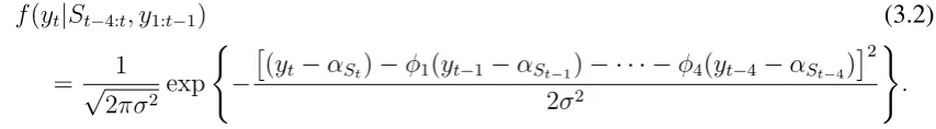
The likelihood function of the model is

f(yt|St−4:t, y1:t−1) (3.2)

= √ 1

2πσ2 exp (

−

(yt−αSt)−φ1(yt−1−αSt−1)− · · · −φ4(yt−4−αSt−4)

2 2σ2

)

.

The state space of {St} is {0,1}, where 0 corresponds to a regime of falling GNP and 1 to

a regime of growing GNP. The analysis is conditional on the parameter estimates given in

Hamilton (1989), who also conditioned posterior state probabilities on those values.

In Hamilton’s analysis, the state at timetis the value that maximises the posterior probability

P[St = st|y1:n], and (implicit) change points into a recession are time points where the state

switches from one to zero. This method for determining states, known as local or posterior

decoding, (Juang and Rabiner 1991; Durbin et al. 1998) is a position specific maximization

algorithm. However, depending on the properties of the transition matrix for St, it does not

necessarily give a complete posterior state sequence that can occur with positive probability.

Determining change points through local decoding neither takes into account the common

def-inition of a recession, which requires at least two quarters of negative growth, nor does it

properly account for the exponential number of possible state sequences and their associated

probabilities.

In the present work, to calculate distributions of changes into recessions, the imbedding state

spaceZ0 is constructed as outlined in Section 2. The value ofk = 2used here corresponds to

the common definition of requiring two quarters of falling GNP for a recession to be confirmed.

The posterior transition probabilitiesP[St=st|St−1 =st−1, . . . , St−r =st−r, y1:n]are used in

the transition probability matrix of the processZt.

[Table 1 about here.]

[Figure 2 about here.]

Figure 2 gives more information about the specific structure of the changes in regime for

GNP. The first thing to note is that the third period of falling GNP may occur with reasonable

probability in two quite different places. This indicates that the variability in assigning the

indicating that regimes of falling GNP could begin and end at two different places. A sustained

period of growth is indicated from the early 1960’s until just before 1970, with little variability

in this assessment, which concurs with the NBER economic thinking about the time period. For

the remainder of the plots in Figure 2, it can be seen that the distribution peaks are still fairly

distinct, meaning that the model is characterising regimes as being either falling or growing

without too much overlap. This assessment concurs with economic thinking on the nature of

the business cycle, in that high frequency oscillations are not likely, and suggests that the model

is still capturing properties of the data even towards the end of the data period. Probabilities

for regime periods are only plotted for cases with at least 0.05 total probability. There is only

a 0.018 chance of there being ten or more periods of falling GNP in the data, so only the first

nine change point distributions are plotted.

[Figure 3 about here.]

Table 1 gives the CPPs according to the model of peaks and troughs of the business cycle

occurring at locations determined by the NBER. As can be seen, the model produces a

quantita-tively good fit for most of the NBER determinations but some NBER peaks are not particularly

probable under the model, especially the second and sixth peaks (both less than 1% chance of

occurring at the NBER date using the model). These two recessions were of particular interest

in the Hamilton (1989) analysis as they were associated with the Suez Crisis and the Iranian

Revolution, respectively. The present analysis shows that the NBER recession dates closest to

these two events likely do not reflect the immediate effect of the two events. It is also

interest-ing to note that while there are two quarters (6 months) difference between the locations of the

NBER peak (1957.III) and the peak in the posterior state probabilities (1957.I) for recession

two, and three quarters difference (NBER: 1980.I, Posterior Decoding: 1979.II) for recession

six, the probability of recession six starting at the NBER point is higher than the probability of

recession two starting at the NBER point. This shows that when trying to determine whether

events are explained by the model, exact CPP are better than using distance from the time of a

peak in the posterior state probabilities for the event of interest. It is also interesting to note that

can be seen in the graph in Figure 2. In addition to the point estimates, interval probabilities of

a change point being at most one quarter different from the NBER dates are also given in Table

1, yielding a confidence interval for the NBER dates in addition to the point probabilities.

Figure 3 shows that the time locations for change points are grouped, although it should be

remembered that this plot, unlike those of Figure 2, is not a distribution over time due to the

multiple regimes in the data, but rather a graph of the CPP at each time point. The probabilities

are moderately peaked, indicating that there are only a few times where change points are likely

to occur. It is of interest to note however from both this graph and those in Figure 2 that the

fourth change point into a recessionary state as determined by Hamilton’s analysis (posterior

decoding) occurs between two peaks (at 1969.III). Thus this is actually an unlikely time (0.18 is

the corresponding probability; see Figure 3) for the change to have occurred, with it being much

more likely to have occurred either just before or just after this date (the NBER peak is just after

that at 1969.IV). In addition, in Figure 3, a comparison is given to computing the probabilities

of change points using a sampling based scheme (of the form indicated in subsection 2.4).

Using an efficient definition of the sample space needed to calculate the exact probabilities,

the effective number of comparative computational samples for the exact method is 40 (using

m = 20). As indicated in Figure 3, even103 _{samples have some fairly large sampling errors,}

while105 samples basically capture all the information (although still with a small amount of

sampling error (e.g. around 1979)).

In addition to the above analysis, distributions concerning the number of regimes or the

length of particular regimes could easily be found (see Section 2 of supplementary material),

which could be used to give further interpretation to the properties of the model.

4. CONCLUDINGREMARKS

In this paper, methods for calculating change point distributions in general finite state HMMs

(or Markov switching models) have been presented. A derived link between waiting time

distri-butions and change point analysis has been exploited to compute probabilities associated with

determined by maximising the conditional probability at each time point of states given the

data can be misleading. As a by-product of deriving the theoretical basis for the approach,

smoothing algorithms in the literature have been investigated and a correction to the algorithm

given in Kim (1994) has been presented in the supplementary material.

Functions of run distributions have been examined. It would be straightforward to extend the

ideas to patterns that are more complex than runs, and to models with multiple regimes. The

definition of change points has been generalised to force a sustained change before a change

point is counted, however the normal definition of change point (settingk = 1and without the

first point being deemed a change point) as a switch from the current regime can be handled by

a slight modification of the methodology, namely by adding a continuation state for the zeroth

occurrence.

If the distribution of the change points is of fundamental interest, and a suitable prior

distri-butionπ(θ)is known for the parametersθ, then a Bayesian approach can be considered:

P[τi =t|y1:n]∝

Z

θ

P[τi =t|y1:n, θ]π(θ)dθ =

Z

θ

P[W(1, i) = t|y1:n, θ]π(θ)dθ. (4.1)

Numerical integration over the parameter space has been used in change point analysis in the

past (Fearnhead and Liu 2007). Equation (4.1) does not include the unknown states explicitly;

they only occur through terms that may easily be computed exactly. Thus state sampling is

not needed, especially if a suitable importance sampling distribution can be found to compute

the integral. Most sampling schemes such as MCMC need the likelihood to include the

un-known states, a much higher dimensional problem than when only the change point times are

considered.

While the distributions given in this paper can be approximated by sampling the unknown

states, there are several disadvantages to this approach. Repeated sampling over the set of

unknown states is computationally expensive and introduces sampling error into the

computa-tions, whereas in the present workP[W(1, i) = t|y1:n, θ], i = 1, . . . , mare calculated exactly,

at a computational complexity equivalent to at most drawing3msamples in the standard change

to approximate the distribution of this higher dimensional space even when the parameters are

known, rendering state sampling approaches unappealing. In addition, the problem of lack of

invariance of change point results under state re-labelling is avoided using the method presented

in this paper.

The CPP point distribution could alternatively be found, without using the techniques

pre-sented here, by finding the posterior distribution of St−max(k,r), . . . , St−1, St using smoothing

techniques similar to the smoother given in the supplementary material, but the computation

time would then be exponential in k. Also, the methodology presented in this paper is

neces-sary if change point distributions for each individual occurrence are required, and in that case

CPP would require no extra computation other than summing probabilities over time points.

All the analysis and computational steps of this paper have been conditioned on the

param-eter values in the model. The effect of paramparam-eter estimation on the distributions calculated has

not been explicitly considered; plug-in MLEs or posterior means have been used, as is often

done with other techniques such as local decoding or the Viterbi algorithm. However, in a small

stability study using asymptotic MLE distributions and Monte Carlo integration for the GNP

data, the CPPs were found to be robust to small fluctuations in the parameter estimates (data

not shown). This was also seen to be the case in Figure 1. In addition, in applications where

the parameters are determined using training data and the model is then applied to test data,

the distributions of the change point locations in the test data are exact, conditional on those

parameters. If MCMC or other techniques were available for efficient parameter estimation

based on sampling the unknown state sequence (e.g. Chib (1998)), it would indeed be possible

to generate posteriors for the parameters and then combine these with the proposed

methodol-ogy to obtain complete distributions without using the sampled state sequences, which may be

slower to converge than the parameter estimates themselves. However, care would need to be

taken given the role of the underlying states in generating the posterior parameter estimates.

It should also be noted that many Markov switching models, such as state space switching

models (Kim 1994), are analysed through the use of approximations to obtain the smoothed

very large when taking advantage of algorithms such as the Kalman filter and also whenr is

not a fixed value but is dependent on the data length (Fr¨uhwirth-Schnatter 2006), for example

in moving average Markov switching models. There have been several suggestions for ways

to implement approximations (Kim 1994; Billio and Monfort 1998) to the likelihood

func-tion in such cases. These techniques can also be used to approximate the smoothed transifunc-tion

probabilities needed in this paper.

In conclusion, methods for further investigation of change points implied by Hidden Markov

models (including Markov switching models) have been presented. The methods are ways of

detecting and evaluating change points that are implied by a model. In addition, formulas are

given to facilitate evaluation of joint and marginal change point distributions. The widespread

use of Markov switching models and change point models in statistics and econometrics, along

with hidden state segmentation models used in computer science, will provide many possible

applications of this work.

ACKNOWLEDGEMENTS

The authors would like to thank the editor, the coordinating editor and a referee for very

helpful comments, including a suggested example, which greatly improved the paper. JA was

supported by the EPSRC (UK) and HEFCE through the CRiSM programme grant and by the

project grant EP/H016856/1. DM was supported by the National Science Foundation under

Grant DMS-0805577.

REFERENCES

Albert, J. H. and S. Chib (1993). Bayes inference via Gibbs sampling of autoregressive time

series subject to Markov mean and variance shifts. Journal of Business and Economic

Statistics 11, 1–15.

Aston, J. A. D. and D. E. K. Martin (2007). Distributions associated with general runs and

patterns in hidden Markov models.Annals of Applied Statistics 1, 585–611.

Balakrishnan, N. and M. Koutras (2002). Runs and Scans with Applications. New York:

Barry, D. and J. A. Hartigan (1992). Product partition models for change point problems.

Annals of Statistics 20, 260–279.

Barry, D. and J. A. Hartigan (1993). A Bayesian analysis for change-point problems.Journal

of the American Statistical Association 88, 309–319.

Billio, M. and A. Monfort (1998). Switching state space models: Likelihood functions,

fil-tering and smoothing.Journal of Statistical Planning and Inference 68, 65–103.

Capp´e, O., E. Moulines, and T. Ryd´en (2005).Inference in Hidden Markov Models. Springer.

Carpenter, J., P. Clifford, and P. Fearnhead (1999). An improved particle filter for non-linear

problems.IEE proceedings - Radar, Sonar and Navigation 146, 2–7.

Chib, S. (1998). Estimation and comparison of multiple change-point models. Journal of

Econometrics 86, 221–241.

Durbin, R., S. Eddy, A. Krogh, and G. Mitchison (1998). Biological Sequence Analysis.

Cambridge University Press.

Eddy, S. R. (2004). What is a hidden Markov model? Nature Biotechnology 22, 1315–1316.

Fearnhead, P. (2006). Exact and efficient Bayesian inference for multiple changepoint

prob-lems.Statistics and Computing 16, 203–213.

Fearnhead, P. and Z. Liu (2007). Online inference for multiple changepoint problems.

Jour-nal of the Royal Statistical Society, Series B 69, 589–605.

Feller, W. (1968). An Introduction to Probability Theory and Its Applications, Volume 1.

John Wiley & Sons.

Fr¨uhwirth-Schnatter, S. (2006).Finite Mixture and Markov Switching Models. Springer.

Fu, J. C. and M. V. Koutras (1994). Distribution theory of runs: A Markov chain approach.

Journal of the American Statistical Association 89, 1050–1058.

Gu´edon, Y. (2007). Exploring the state sequence space for hidden Markov and semi-Markov

chains.Computational Statistics and Data Analysis 51, 2379–2409.

Gu´edon, Y. (2008). Exploring the segmentation space for the assessment of multiple

Hamilton, J. D. (1989). A new approach to the economic analysis of nonstationary time

series and the business cycle.Econometrica 57, 357–384.

Juang, B. H. and L. R. Rabiner (1991). Hidden Markov models for speech recognition.

Technometrics 33, 251–272.

Kim, C.-J. (1994). Dynamic linear models with Markov-switching. Journal of

Economet-rics 60, 1–22.

Kschischang, F. R., B. J. Frey, and H.-A. Loeliger (2001). Factor graphs and the sum-product

algorithm.IEEE Transactions on Information Theory 47, 498–519.

MacDonald, I. L. and W. Zucchini (1997). Hidden Markov and Other Models for

Discrete-valued Time Series. London, UK: Chapman & Hall.

Martin, A. D., K. M. Quinn, and J. H. Park (2011). MCMCpack: Markov Chain Monte Carlo

in R.Journal of Statistical Software 42(9), 1–22.

R Development Core Team (2011).R: A Language and Environment for Statistical

Comput-ing. Vienna, Austria: R Foundation for Statistical Computing. ISBN 3-900051-07-0.

Rabiner, L. R. (1989). A tutorial on hidden Markov models and selected applications in

speech recognition.Proceedings of the IEEE 77, 257–286.

Sims, C. A. and T. Zha (2006). Were there regime switches in US monetary policy?

Ameri-can Economic Review 96, 54–81.

Viterbi, A. (1967). Error bounds for convolution codes and an asymptotically optimal

de-coding algorithm.IEEE Transactions on Information Theory 13, 260–269.

ADDRESS FORCORRESPONDENCE: JOHNASTON

CRISM TEL:+44-24-7657-4808

DEPARTMENT OFSTATISTICS FAX:+44-24-7652-4532

UNIVERSITY OFWARWICK EMAIL: J.A.D.A S T O N@W A R W I C K.A C.U K

FIGURE1. Change point distributions calculated using different approaches for Chib’s (1998) binary change point model. In each graph the blue area gives the

distribution of the time of the first change point and the red line the

distribu-tion of the time of the second change point. Top: Distribudistribu-tion of change points

calculated using the posterior mean of the parameters. Middle: Distribution of

change points calculated by finding the distribution of change points for each

parameter set with the MCMC run and then pointwise averaging the

distribu-tions. Bottom: Distribution of Change points calculated by determining the

FIGURE 2. Regime Variability of GNP. This is a graphical plot to detect the variability of when different periods of falling GNP states occur in GNP data

from 1951:II to 1984:IV. The numbers in the legends to the right of the graphs

indicate the index of the period of falling GNP under consideration, followed

by the probability of at least that many periods occurring by the end of the data.

The very top graph gives a plot of the logged differenced GNP data along with

the start (blue line) and finish (red line) of periods whereP[St = 0|y1:n]>0.5.

For the subsequent graphs, the blue area indicates the distribution of the start of

a period of falling GNP while the red line indicates the distribution of the end

of the falling GNP regime, thus giving a measure of the variability in the length

of periods of falling GNP. Theith graph gives the distribution of theith falling

GNP period having occurred at timet, fori= 1, . . . , m. The final plot gives the

(a) GNP Change Point Probabilities (k= 2)

(b) Differences from Exact Probabilities using Sample Based Methods

FIGURE 3. (a) Plot of the CPP of starting (CPP0) or ending (CPPe0) a falling

GNP regime within the time period 1951:II to 1984:IV. The graph, while not a

distribution, gives information as to the probability of a switch occurring in a

particular quarter. (b) This graph indicates the precision of obtaining the same

information for CPP0 through a sampling based estimation scheme for various

TABLE1. Dating of the US business cycle peaks and troughs as determined by

the NBER, along with their associated probabilities of occurring at or before

each time according to the AR(4) mean switching model.

i Peak (t1) P[W0(2, i) =t1+1] CPP0(t1,2) CPP0 Trough (t2) P[W0e(2, i) =t2] CPPe0(t2,2) CPPe0

(t1−1 :t1+1,2) (t2−1 :t2+1,2)

1 1953.III 0.46 0.47 0.93 1954.II 0.72 0.73 0.99

2 1957.III 0.0036 0.0092 0.58 1958.II 0.13 0.18 0.99

3 1960.II 0.66 0.83 0.85 1961.I 0.034 0.042 0.87

4 1969.IV 0.2 0.33 0.89 1970.IV 0.44 0.71 0.72

5 1973.IV 0.065 0.1 0.45 1975.I 0.48 0.8 0.98

6 1980.I 0.0088 0.019 0.37 1980.III 0.2 0.42 0.85