University of Warwick institutional repository: http://go.warwick.ac.uk/wrap
This paper is made available online in accordance with
publisher policies. Please scroll down to view the document
itself. Please refer to the repository record for this item and our
policy information available from the repository home page for
further information.
To see the final version of this paper please visit the publisher’s website.
Access to the published version may require a subscription.
Author(s): Celik, T. and Tjahjadi, T.
Article Title: Automatic Image Equalization and Contrast Enhancement
Using Gaussian Mixture Modeling
Year of publication: 2012
Link to published article:
http://dx.doi.org/10.1109/TIP.2011.2162419
Publisher statement: “© 2012 IEEE. Personal use of this material is
permitted. Permission from IEEE must be obtained for all other uses, in
any current or future media, including reprinting/republishing this
material for advertising or promotional purposes, creating new
collective works, for resale or redistribution to servers or lists, or reuse
of any copyrighted component of this work in other works.”
Citation: Celik, T and Tjahjadi, T. (2012). Automatic Image Equalization
and Contrast Enhancement Using Gaussian Mixture Modeling.
Automatic Image Equalization and Contrast
Enhancement Using Gaussian Mixture Modelling
Turgay Celik and Tardi Tjahjadi Senior Member, IEEE
Abstract
In this paper, we propose an adaptive image equalization algorithm which automatically enhances the contrast in an input
image. The algorithm uses Gaussian mixture model (GMM) to model the image grey-level distribution, and the intersection points
of the Gaussian components in the model are used to partition the dynamic range of the image into input grey-level intervals.
The contrast equalized image is generated by transforming the pixels’ grey levels in each input interval to the appropriate output
grey-level interval according to the dominant Gaussian component and cumulative distribution function (CDF) of the input interval.
To take account of human perception the Gaussian components with small variances are weighted with smaller values than the
Gaussian components with larger variances, and the grey-level distribution is also used to weight the components in the mapping
of the input interval to the output interval. Experimental results show that the proposed algorithm produces better or comparable
enhanced images than several state-of-the-art algorithms. Unlike the other algorithms, the proposed algorithm is free of parameter
setting for a given dynamic range of the enhanced image and can be applied to a wide range of image types.
Index Terms
Contrast enhancement, histogram equalization, normal distribution, Gaussian mixture modelling, histogram partition.
I. INTRODUCTION
The objective of an image enhancement technique is to bring out hidden image details, or to increase the contrast of an
image with low dynamic range [1]. Such a technique produces an output image that subjectively looks better than the original
image by increasing the grey level differences (i.e., the contrast) among objects and background. Numerous enhancement
techniques have been introduced and these can be divided into three groups: 1) techniques that decompose an image into
high and low frequency signals for manipulation [2], [3]; 2) transform-based techniques [4]; and 3) histogram modification
techniques [5]–[16].
Techniques in the first two groups often use multiscale analysis to decompose the image into different frequency bands and
enhance its desired global and local frequencies [2]–[4]. These techniques are computationally complex but enable global and
local contrast enhancement simultaneously by transforming the signals in the appropriate bands or scales. Furthermore they
require appropriate parameter settings which might otherwise result in image degradations. For example, the centre-surround
Retinex [2] algorithm was developed to attain lightness and colour constancy for machine vision applications. The constancy
refers to the resilience of perceived colour and lightness to spatial and spectral illumination variations. The benefits of the
Retinex algorithm include dynamic range compression and colour independence from the spatial distribution of the scene
This work was supported by the Warwick University Vice Chancellor Scholarship.
Turgay Celik and Tardi Tjahjadi are with the School of Engineering, University of Warwick, Gibbet Hill Road, Coventry, CV4 7AL, United Kingdom.
illumination. However, this algorithm can result in “halo” artefacts, especially in boundaries between large uniform regions.
Also, a “greying out” can occur, in which the scene tends to change to middle grey.
Among the three groups the third group received the most attention due to their straightforward and intuitive implementation
qualities. Linear contrast stretching (LCS) and global histogram equalization (GHE) are two widely utilized methods for global
image enhancement [1]. The former linearly adjusts the dynamic range of an image, and the latter uses an input-to-output
mapping obtained from the cumulative distribution function (CDF) which is the integral of the image histogram. Since the
contrast gain is proportional to the height of the histogram, grey levels with large pixel populations are expanded to a larger
range of grey levels while other grey-level ranges with fewer pixels are compressed to smaller ranges. Although GHE can
efficiently utilize display intensities, it tends to over-enhance the image contrast if there are high peaks in the histogram, often
resulting in a harsh and noisy appearance of the output image. LCS and GHE are simple transformations but they do not
always produce good results, especially for images with large spatial variation in contrast. In addition, GHE has the undesired
effect of over-emphasizing any noise in an image.
In order to overcome the aforementioned problems, local histogram equalization (LHE) based enhancement techniques have
been proposed, e.g., [5], [6]. The LHE method [6] uses a small window that slides through every image pixel sequentially and
only pixels within the current position of the window are histogram equalized, and the grey-level mapping for enhancement is
done only for the centre pixel of the window. Thus, it utilises local information. However, LHE sometimes causes
over-enhancement in some portion of the image and enhances any noise in the input image along with the image features.
Furthermore, LHE based methods produce undesirable checkerboard effects.
Histogram Specification (HS) [1] is a method that uses a desired histogram to modify the expected output image histogram.
However, specifying the output histogram is not a straightforward task as it varies from image to image. The Dynamic Histogram
Specification (DHS) [7] generates the specified histogram dynamically from the input image. In order to retain the original
histogram features, DHS extracts the differential information from the input histogram and incorporates extra parameters to
control the enhancement such as the image original and the resultant gain control values. However, the degree of enhancement
achievable is not significant.
Some researches have also focused on improving histogram equalization based contrast enhancement such as mean preserving
bi-histogram equalization (BBHE) [8], equal area dualistic sub-image histogram equalization (DSIHE) [9] and minimum mean
brightness error bi-histogram equalization (MMBEBHE) [10]. BBHE first divides the image histogram into two parts with the
average grey level of the input image pixels as the separation intensity. The two histograms are then independently equalized.
The method attempts to solve the brightness preservation problem. DSIHE uses entropy for histogram separation. MMBEBHE
is the extension of BBHE that provides maximal brightness preservation. Although these methods can achieve good contrast
enhancement, they also generate annoying side effects depending on the variation in the grey-level distribution [7]. Recursive
Mean-Separate Histogram Equalization (RMSHE) [11] is another improvement of BBHE. However, it is also not free from side
effects. Dynamic histogram equalization (DHE) [12] first smooths the input histogram by using a one dimensional smoothing
filter. The smoothed histogram is partitioned into histograms based on the local minima. Prior to equalizing the
sub-histograms, each sub-histogram is mapped into a new dynamic range. The mapping is a function of the number of pixels in
each sub-histogram, thus a sub-histogram with a larger number of pixels will occupy a bigger portion of the dynamic range.
However, DHE does not place any constraint on maintaining the mean brightness of the image. Furthermore, several parameters
are used that require appropriate setting for different images.
equalisation with maximum entropy (BPHEME) [13] defines the ideal histogram to have maximum entropy with brightness
preservation. The target histogram which has the maximum differential entropy under the mean brightness constraint is
obtained using variational approach [13]. BPHEME is designed to achieve maximum entropy. Although entropy maximisation
corresponds to contrast stretching to some extent, it is not a straightforward consequence and does not definitely lead to contrast
enhancement [14]. In flattest histogram specification with accurate brightness preservation (FHSABP) [14], convex optimisation
is used to transform the image histogram into the flattest histogram, subject to a mean brightness constraint. An exact histogram
specification method is used to preserve the image brightness. However, when the grey levels of the input image are equally
distributed, FHSABP behaves very similar to GHE. Furthermore, it is designed to preserve the average brightness which may
produce low contrast results when the average brightness is either too low or too high. In histogram modification framework
(HMF) which is based on histogram equalization, contrast enhancement is treated as an optimization problem that minimizes a
cost function [15]. Penalty terms are introduced in the optimisation in order to handle noise and black/white stretching. HMF
can achieve different levels of contrast enhancement, through the use of different adaptive parameters. These parameters have
to be manually tuned according to the image content to achieve high contrast. In order to design a parameter free contrast
enhancement method, genetic algorithm (GA) is employed to find a target histogram which maximizes a contrast measure
based on edge information [16]. We call this method contrast enhancement based on GA (CEBGA). CEBGA suffers from the
drawbacks of GA based methods, namely dependency on initialization and convergence to a local optimum. Furthermore, the
mapping to the target histogram is scored by only maximum contrast which is measured according to average edge strength
estimated from the gradient information. Thus, CEBGA may produce results which are not spatially smooth. Finally, the
convergence time is proportional to the number of distinct grey levels of the input image.
The aforementioned techniques may create problems when enhancing a sequence of images, or when the histogram has
spikes, or when a natural looking enhanced image is required. In this paper, we propose an adaptive image equalization
algorithm which is effective in terms of improving visual quality of different types of input images. Images with low-contrast
are automatically improved in terms of an increase in dynamic range. Images with sufficiently high contrast are also improved
but not as much. The algorithm further enhances the colour quality of the input images in terms of colour consistency, higher
contrast between foreground and background objects, larger dynamic range and more details in image contents. The proposed
algorithm is free from parameter setting. Instead the pixel values of an input image are modelled using Gaussian mixture model
(GMM). The intersection points of the Gaussians in the model are used in partitioning the dynamic range of the input image
into input grey-level intervals. The grey level of the pixels in each input interval are transformed according to the dominant
Gaussian component and the CDF of the interval to obtain the contrast equalized image.
The paper is organized as follows. Section II presents the proposed automatic image equalization algorithm and the necessary
background related to the GMM fit of the input image data. Section III presents the subjective and quantitative comparisons
of the proposed method with several state-of-the-art enhancement techniques. Section IV concludes the paper.
II. PROPOSEDALGORITHM
Let us consider an input image, X={x(i, j) |1 ≤i≤H,1 ≤j ≤W}, of size H×W pixels, wherex(i, j)∈R. Let us assume that Xhas a dynamic range of[xd, xu]wherex(i, j)∈[xd, xu]. The main objective of the proposed algorithm is to generate an enhanced image, Y ={y(i, j) |1 ≤i ≤H,1 ≤j ≤W}, which has a better visual quality with respect to
A. Modelling
The Gaussian mixture model (GMM) can model any data distribution in terms of a linear mixture of different Gaussian
distributions with different parameters. Each of the Gaussian components has a different mean, standard deviation and proportion
(or weight) in the mixture model. A Gaussian component with a low standard deviation and a large weight represents compact
data with a dense distribution around the mean value of the component. When the standard deviation becomes larger, the data
is dispersed about its mean value. The human eye is not sensitive to small variations around dense data, but is more sensitive
to widely scattered fluctuations. Thus, in order to increase the contrast while retaining image details, dense data with low
standard deviation should be dispersed while scattered data with high standard deviation should be compacted. This operation
should be done so that the grey-level distribution is retained. In order to achieve this, we use GMM to partition the distribution
of the input image into a mixture of different Gaussian components.
The grey-level distributionp(x), wherex∈X, of the input imageXcan be modelled as a density function composed of a linear combination ofN functions using the GMM [17], i.e.,
p(x) =
N
X
n=1
P(wn)p(x|wn), (1)
wherep(x|wn)is thenth component density, andP(wn)is the prior probability of the data points generated from component wn of the mixture. The component density functions are constrained to be Gaussian distribution functions, i.e.,
p(x|wn) =p 1
2πσ2 wn
exp −(x−µwn)
2
2σ2 wn
!
, (2)
where µwn and σ2
wn are respectively the mean and the variance of the nth component. Each of the Gaussian distribution functions satisfies the constraint
Z ∞
−∞
p(x|wn)dx= 1, (3)
and the prior probabilities are chosen to satisfy the constraints
N
X
n=1
P(wn) = 1 and 0≤P(wn)≤1. (4)
A GMM is completely specified by its parametersθ=P(wn), µwn, σ2wn N
n=1. The estimation of the probability distribution
function (PDF) of an input image data x reduces to finding the appropriate values of θ. In order to estimate θ, maximum likelihood estimation (MLE) techniques such as the expectation maximization (EM) algorithm [18] have been widely used.
Assuming the data points X={x1, x2, . . . , xH×W} are independent, the likelihood of the dataX is computed by
L(X;θ) =
H×W
Y
k=1
p(xk;θ) (5)
given the distribution or, more specifically, given the distribution parameters θ. The goal of the estimation is to find θˆ that
maximizes the likelihood, i.e.,
ˆ
θ= argmax
θ
L(X;θ). (6)
Instead of maximizing this function directly, the log-likelihoodL(X;θ) = lnL(X;θ)≡PH×W
k=1 p(xk;θ)is used because it is analytically easier to handle.
The EM algorithm starts from an initial guess θ0 for the distribution parameters and the log-likelihood is guaranteed to
(a)
0 50 100 150 200 250
0 0.005 0.01 0.015 0.02 0.025 0.03
x
p(x)
Histogram P(w
1) p(x|w1) P(w
2) p(x|w2) P(w
3) p(x|w3) P(w
4) p(x|w4) p(x) (GMM)
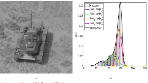
[image:6.612.56.555.52.332.2](b)
Fig. 1. (a) A grey-level image; and (b) its histogram and GMM fit.
estimates, which is true particularly for Gaussian mixture distributions with arbitrary covariance matrices. The initialization is
one of the problems of the EM algorithm. The selection of θ0 (partly) determines where the algorithm converges or hits the
boundary of the parameter space to produce singular, meaningless results. Furthermore, the EM algorithm requires the user to
set the number of components, and the number is fixed during the estimation process.
The Figueiredo-Jain (FJ) algorithm [19] which is an improved variant of the EM algorithm overcomes major weaknesses of
the basic EM algorithm. The FJ algorithm adjusts the number of components during estimation by annihilating components
that are not supported by the data. It avoids the boundary when it annihilates components that are becoming singular. It is also
allowed to start with an arbitrarily large number of components, which addresses the initialization of the EM algorithm. The
initial guesses for component means can be distributed into the whole space occupied by the training samples, even setting one
component for every single training sample. Due to its advantages over EM algorithm, in this work we adopt the FJ algorithm
for parameter estimation.
Fig. 1(a) and (b) respectively illustrate an input image and its histogram together with its GMM fit. The histogram is modelled
using four Gaussian components, i.e., N = 4. The close match between the histogram (shown as rectangular vertical bars) and GMM fit (shown as solid black line) is obtained using FJ algorithm. There are three main grey tones in the input image
corresponding to the tank, its shadow and the image background. The other grey-level tones are distributed around the three
main tones. However, FJ algorithm results in four Gaussian components (N = 4) for the mixture model. This is because the
grey tone with the highest average grey value corresponding to the image background has a deviation too large for a single
Gaussian component to represent it. Thus it is represented by two Gaussian components, i.e.,w3andw4as shown in Fig. 1(b). All intersection points between Gaussian components that fall within the dynamic range of the input image are denoted by
yellow circles, and significant intersection points that are used in dynamic range representation are denoted by black circles.
There is only one dominant Gaussian component between two intersection points, which adequately represents the data within
TABLE I
THE NUMERICAL VALUES OF INTERSECTION POINTS DENOTED BY YELLOW CIRCLES INFIG. 1(B)BETWEEN COMPONENTS OFGMMFIT TO THE
GREY-LEVEL IMAGE SHOWN INFIG. 1(A).
GMM Components
w1 w2 w3 w4
w1 - -718.88, 90.05 115.18, 225.52 129.46, 193.08
w2 -718.88, 90.05 - 129.75, 172.39 141.31, 168.18
w3 115.18, 225.52 129.75, 172.39 - 149.82, 163.54
w4 129.46, 193.08 141.31, 168.18 149.82, 163.54
-componentw1 (shown as solid blue line). Thus the data within each interval is represented by a single Gaussian component which is dominant with respect to the other components. The dynamic range of the input image is represented by the union
of all intervals.
B. Partitioning
The significant intersection points are selected from all the possible intersections between the Gaussian components. The
intersection points between two Gaussian componentswmandwn are found by solving
P(wm)p(x|wm) =P(wn)p(x|wn), (7)
or equivalently
−(x−µwm)
2
2σ2 wm
+(x−µwn) 2
2σ2 wn
= ln
P(wn)
P(wm)
σwm σwn
, (8)
which results in
ax2+bx+c= 0, (9)
where
a= σ2wm−σ 2 wn
, b= 2 µwmσw2n−µwnσ 2 wm
,
c= µ2 wnσ
2 wm −µ
2 wmσ
2 wn
−2σ2
wmσ 2 wnln
P(wn)
P(wm)
σwm σwn
.
The second order parametric equation Eq. (9) has two roots, i.e.,
x(1)m,n= −
b+√b2−4ac
2a , x
(2) m,n= −
b−√b2−4ac
2a . (10)
In Fig. 1(b) all intersection points between GMM components are denoted by yellow circles. The numerical values of the
intersection points determined using Eq. (10) are shown in Table I. Table I is symmetric, i.e., the intersection points between
the componentsw1 andw2are the same as the intersection points between componentsw2 andw1. The intersection points of two components are independent of the order of the components. All possible intersection points that are within the dynamic
range of the image are detected. The leftmost intersection point between componentsw1 andw2 is at −718.88which is not within the dynamic range of the input image, thus it could not be considered. In order to allow combination of intersection
The total number of intersection points calculated is N(N−1). The significant intersection points x(d)s , where d ∈
{1, . . . , D},D≤N(N−1), are selected among all intersection points. For a given intersection pointx(k)m,n, wherek={1,2}, between Gaussian componentswmandwn it is selected as a significant intersection point if and only if it is a real number in the dynamic range of the input image, i.e., x(k)m,n∈X, and the Gaussian componentswmandwn contain the maximum value in the mixture for the point x(k)m,n, i.e.,
P(wm)px(k)m,n|wm
=P(wn)px(k)m,n|wn
, (11)
P(wm)px(k)m,n|wm
> P(wk)px(k)m,n|wk
, (12)
where∀wk 6={wm, wn}.
The significant intersection points are sorted in ascending order of their value and are partitioned into grey-level intervals
to cover the entire dynamic range ofX, i.e.,x∈xs=hx(l)s , x(1)s
i
∪hx(1)s , x(2)s
i
· · · ∪ · · ·hx(D)s , x(r)s
i
. The leftmost significant
intersection pointx(l)s is selected as the value of xfor which
x(l)s =x, F(x)≥ Th
HW, F(x−∆)< Th
HW, (13)
where the minimum distance between two consecutive numbers is∆, e.g.,∆ = 1in the case of 8-bit input imageXconsidered
in this work,F(x)is the CDF ofx, andThis the minimum number of pixels which will be excluded from the tails of the grey-level distribution of x. To consider all pixel grey values of Xwe set Th= 1. Similarly, the rightmost significant intersection pointx(r)s is selected by considering the tail of the grey-level distribution ofxfor which
x(r)s =x, (1−F(x))≥ Th
HW, (1−F(x+ ∆))< Th
HW. (14)
The significant intersection points that fall outside of the intervalhx(l)s , x(r)s
i
are ignored since they are the intersection points
between two Gaussian components that fall outside the dynamic range of X, andxsis updated asxs=hx(1)s , x(2)s , . . . , x(K)s
i
withx(1)s < x(2)s < . . . < x(K)s , whereKis the maximum number of significant intersection points. In Fig. 1 the six significant intersection points are denoted by black circles, and the range ofxscovers the entire dynamic range of X.
The CDF of xis
F(x) =
Z x
−∞
p(x)dx=
Z x
−∞
N
X
n=1
P(wn)p(x|wn)dx
=
N
X
n=1 P(wn)
Z x
−∞
1
p
2πσ2 wn
exp−(x−µwn) 2
2σ2 wn dx = N X n=1 P(wn)
Z (x√−µwn)
2σwn
−∞
1
√πexp −t2
dt. (15)
It can be calculated using the closed form expression
F(x) =
N
X
n=1
P(wn)Fwn(x), (16)
whereFwn(x)is the CDF of Gaussian componentwn, and using the definition of the error function (erf(x)) (also called the Gauss error function) [20] it is computed as Fwn(x) =βx√−µwn
2σwn
, whereβ(x) is computed in terms of error function [20] as follows:
β(x) =
(1 +erf(x))/2 , iffx≥0
(1−erf(|x|))/2 , otherwise,
where the numerical values of erf(x) are tabulated in [20]. The function β(x) is invertible, i.e., for a given β(x) = a, x=β−1(a)exists.
The consecutive pairs of significant intersection points are used to partition the dynamic range of Xinto subintervals, i.e.,
[xd, xu] =hx(1)s , x(2)s
i
∪hx(2)s , x(3)s
i
∪· · ·∪hx(Ks −2), x(Ks −1)
i
∪hx(Ks −1), x(K)s
i
. The subintervalhx(k)s , x(k+1)s
i
is represented by
a Gaussian componentwk which is dominant with respect to the other Gaussian components in the subinterval. The dominant Gaussian component is found by considering the a posteriori probability of each component in the interval hx(k)s , x(k+1)s
i
which is equivalent to the area under the Gaussian component, i.e.,
wk= argmax
∀wi
h
Fwi
x(k+1)s
−Fwi
x(k)s
i
. (18)
C. Mapping
The interval hx(k)s , x(k+1)s
i
, where k = 1,2, . . . , K−1, in xs is mapped onto the dynamic range of the output image
Y. In the mapping, each interval covers a certain range which is proportional to a weight αk, where αk ∈[0,1], which is calculated by considering two figure of merits simultaneously: 1) the rate of the total number of pixels that fall into the interval
h
x(k)s , x(k+1)s
i
; and 2) the standard deviation of the dominant Gaussian componentwk, i.e.,
αk= (σwk)
γ
PN
i=1(σwi) γ
h
Fx(k+1)s
−Fx(k)s
i
PK−1 i=1
h
Fx(i+1)s
−Fx(i)s
i. (19)
The first term adjusts the brightness of the equalized image, and γ ∈ [0,1] is brightness constant (in this paperγ = 0.5 is used). The lower the value of γ, the brighter is the output image. The second term in Eq. (19) is related to the grey-level distribution and is used to retain the overall content of the data in the interval. Eq. (19) maintains a balance between the data
distribution and variance of the data in a certain interval. Since the human eye is more sensitive to sudden changes in widely
scattered data and less sensitive to smooth changes in densely scattered data, Eq. (19) gives larger weights to widely scattered
data (larger variance), and vice versa.
Usingαk, the input intervalhx(k)s , x (k+1) s
i
is mapped onto the output intervaly(k), y(k+1)
according to
y(k) = yd+ (yu−yd)
k−1
X
i=1
αi, (20)
y(k+1) = y(k)+αk(yu−yd).
The above mapping guarantees that the output dynamic range is covered by the mapping, i.e., [yd, yu] =
y(1)=yd, y(2) ∪
y(2), y(3)
∪ · · · ∪
y(K−1), y(K)=yu
.
In the final mapping of pixel values from the input interval onto the output interval, the CDF of the distribution in the output
interval is preserved. Let Gaussian distribution wk′ with parameters µw
k′ andσ
2
wk′ represent the Gaussian componentwk in
the rangey(k), y(k+1)
. The parametersµwk′ andσ
2
wk′ are found by solving the following equations simultaneously
Fwkx(k) s
= Fwk′
y(k), (21)
Fwk
x(k+1)s
= Fwk′
y(k+1), (22)
so that the area under the Gaussian distributionwk betweenhx(k)s , x (k+1) s
i
wk′ in the interval
y(k), y(k+1)
. Using Eq. (17) together with equations Eq. (21) and Eq. (22), one can write
β x (k) s −µwk
√
2σwk
!
= β y
(k)−µw k′
√
2σwk′ !
(23)
β x (k+1) s −µwk
√
2σwk
!
= β y
(k+1)
−µwk′
√
2σwk′ !
, (24)
which is equivalent to
x(k)s −µwk
√
2σwk
= y
(k)
−µwk′
√
2σwk′
(25)
x(k+1)s −µwk
√
2σwk
= y
(k+1)
−µwk′
√
2σwk′
. (26)
Using equations Eq. (25) and Eq. (26), the parameters of Gaussian distribution wk′ are computed as follows:
µwk′ =
x(sk)−µwk x(sk+1)−µwky
(k+1)−y(k)
x(sk)−µwk x(sk+1)−µwk −1
(27)
σwk′ =
y(k)−µw k′
x(k)s −µwk
σwk. (28)
The mapping of x to y, where x ∈ hx(k)s , x (k+1) s
i
and y ∈
y(k), y(k+1)
, is achieved by keeping the CDFs of Gaussian
distributionwk and Gaussian distributionwk′ equal, i.e.,
β
x−µwk
√
2σwk
−β x
(k) s −µwk
√
2σwk
!
=
β y−µwk′
√
2σwk′ !
−β y
(k)
−µwk′
√
2σwk′ !
, (29)
where using the equality in Eq. (23),
β
x−µwk
√
2σwk
=β y−µwk′
√
2σwk′ !
⇒ x−µwk
√
2σwk
= y−µwk′
√
2σwk′
results in the following mapping of givenxto the correspondingy according to the Gaussian distributionswk andwk′
y=
x
−µwk
σwk
σwk′ +µwk′. (30)
The final mapping fromxtoyis achieved by considering all Gaussian components in the GMM to retain the pixel distributions in input and output intervals equal. Using the superposition of distributions together with Eq. (30) one can find
y=
N
X
i=1
x−µwi σwi
σwi′ +µwi′
Pwi. (31)
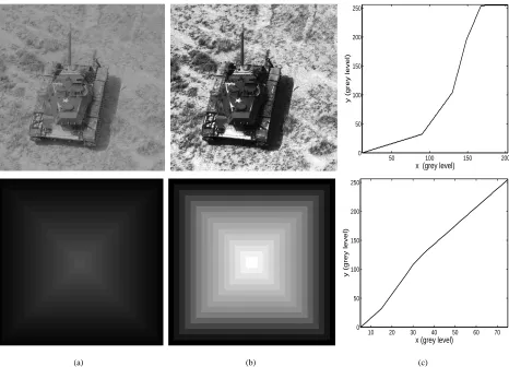
Fig. 2(a), (b) and (c) respectively show the input images, equalized images using the proposed algorithm where the dynamic
range of the output image is [yd, yu] = [0,255], and the mappings between input image data points(x)and equalized output image data points (y)are according to Eq. (31). Fig. 2(c) shows that a different mapping is applied to a different input grey-level interval. Fig. 2(b) shows that the proposed algorithm increases the brightness of the input image while keeping the high
contrast between object boundaries. The input image in the second row of Fig. 2(a) has only fifteen different grey levels, thus
it is difficult to observe the image features. The proposed algorithm linearly transforms the grey levels as shown in Fig. 2(c)
50 100 150 200 0
50 100 150 200 250
x (grey level)
y (grey level)
(a) (b)
10 20 30 40 50 60 70 0
50 100 150 200 250
x (grey level)
y (grey level)
[image:11.612.73.539.51.387.2](c)
Fig. 2. (a) A grey-level input imageX; (b) The equalized output imageYusing the proposed algorithm; and (c) The data mapping between the input and
output images.
One approach to extend the grey-scale contrast enhancement to colour images is to apply the method to their luminance
component only and preserve the chrominance components. Another is to multiply the chrominance values with the ratio of
their input and output luminance values to preserve the hue. The former approach is employed in this paper where an input RGB
image is transformed to CIEL∗a∗b∗colour space [1] and the luminance componentL∗is processed for contrast enhancement. The inverse transformation is then applied to obtain the contrast enhanced RGB image.
III. EXPERIMENTALRESULTS
A dataset comprising standard test images from [21]–[24] is used to evaluate and compare the proposed algorithm with our
implementations of GHE [1], BPHEME [13], FHSABP [14], CEBGA [16] and the weighted histogram approximation of HMF
[15]. GHE, BPHEME, FHSABP and CEBGA are free of parameter selection but HMF requires parameter tuning which is
manually selected according the input test images. It is worth to note that for FHSABP method exact histogram specification
is used [14] to achieve high degree of brightness preservation between input and output images. The test images show wide
variations in terms of average image intensity and contrast. Thus they are suitable for measuring the strength of a contrast
enhancement algorithm under different circumstances.
An output image is considered to have been enhanced over the input image if it enables the image details to be better perceived.
An assessment of image enhancement is not an easy task as an improved perception is difficult to quantify. Nevertheless, in
defines a good measure of enhancement. We use absolute mean brightness error (AMBE) [10], discrete entropy (DE) [25], and
edge based contrast measure (EBCM) [26] as quantitative measures. For colour images, the contrast enhancement is quantified
by computing these measures on their luminance channelL∗ only.
AMBE is the absolute difference between the mean values of an input image Xand output imageY, i.e.,
AM BE(X,Y) =|M B(X)−M B(Y)|, (32)
where M B(X) andM B(Y)are the mean brightness values of X andY, respectively. The lower the value of AMBE, the better is the brightness preservation.
The discrete entropy DE of an imageXmeasures its content, where a higher value indicates an image with richer details.
It is defined as
DE(X) =−
255
X
i=0
p(xi) log (p(xi)), (33)
wherep(xi)is the probability of pixel intensityxi which is estimated from the normalized histogram.
The edge based contrast measure EBCM is based on the observation that the human perception mechanisms are very sensitive
to contours (or edges) [26]. The grey level corresponding to object frontiers is obtained by computing the average value of the
pixel grey levels weighted by their edge values. The contrastc(i, j)for a pixel of an imageXlocated at(i, j)is thus defined as
c(i, j) = |x(i, j)−e(i, j)|
|x(i, j) +e(i, j)|,
where the mean edge grey level is
e(i, j) = X
(k,l)∈N(i,j)
g(k, l)x(k, l). X
(k,l)∈N(i,j) g(k, l),
N(i, j) is the set of all neighbouring pixels of pixel (i, j), and g(k, l) is the edge value at pixel (k, l). Without loss of generality we employ 3×3 neighbourhood, andg(k, l)is computed using the magnitude of the gradient which is estimated from horizontal and vertical Sobel operators [1]. EBCM for image Xis thus computed as the average contrast value, i.e.,
EBCM(X) =
H
X
i=1 W
X
j=1
c(i, j).H×W . (34)
It is expected that for an output image Y of an input imageX, the contrast is improved whenEBCM(Y)≥EBCM(X).
A. Qualitative Assessment
1) Grey-Scale Images: Some contrast enhancement results on grey-scale images are shown in Fig. 3, Fig. 4, Fig. 5 and
Fig. 6. The mapping functions used are shown in Fig. 7 (a)-(d), respectively.
The input image in Fig. 3 shows a firework display [21], and comprises very bright and dark objects. GHE has increased
the overall brightness of the image, but the increase in contrast is not significant and the washout effect is apparent. Both
the darker and brighter regions become even brighter. This is verified by the mapping function in Fig. 7(a) which maps input
grey-level 0 to output grey-level 105. BPHEME and FHSABP preserve the input image average brightness value of 18. This
results in the output image with very low brightness, and thus the contrast enhancement is not noticeable. The mapping function
verifies this observation where the low output brightness and non-linear mapping from input to output are apparent. It is also
clear from the mapping function that BPHEME performs almost one to one mapping when it is compared with the mapping
(a) (b) (c) (d)
(e) (f) (g)
Fig. 3. Contrast enhancement results for image Fireworks: (a) original image; (b) GHE; (c) BPHEME; (d) FHSABP; (e) HMF; (f) CEBGA; and (g) proposed.
(a) (b) (c) (d)
[image:13.612.55.557.54.282.2](e) (f) (g)
Fig. 4. Contrast enhancement results for image Island: (a) original image; (b) GHE; (c) BPHEME; (d) FHSABP; (e) HMF; (f) CEBGA; and (g) proposed.
entropy. Thus, the mapping function of BPHEME achieves almost one-to-one mapping between input and output to guarantee
the maximum entropy. The result of HMF is visually pleasing, providing high contrast as well as a high dynamic range.
However, there are two different spark clusters due to the fireworks and the smoke between sparks. HMF over enhances the
brighter pixels of the sparks and the surrounding smoke, so that the smoke pixels are also identified as spark pixels. This over
enhancement is represented as a sharp change in the mapping function. Furthermore, due to over enhancement of the brighter
pixels, the sparks due to the fireworks cannot be clearly differentiated. The over enhancement is due to forming a histogram
from pixels with significant grey-level differences with their neighbours. The smoke around the sparks has similar but lower
grey-level values. Thus, most of the smoke pixels cannot be differentiated from the spark pixels which results in mapping
them to the same output grey-levels as that of the spark pixels. Due to the not sharp image details caused by the smoke from
[image:13.612.54.561.316.530.2](a) (b) (c) (d)
[image:14.612.53.559.65.364.2](e) (f) (g)
Fig. 5. Contrast enhancement results for image City: (a) original image; (b) GHE; (c) BPHEME; (d) FHSABP; (e) HMF; (f) CEBGA; and (g) proposed.
(a) (b) (c) (d)
(e) (f) (g)
[image:14.612.56.558.424.713.2]0 50 100 150 200 250 0 50 100 150 200 250
x (grey level)
y (grey level)
(a)
0 50 100 150 200 250 0 50 100 150 200 250
x (grey level)
y (grey level)
(b)
50 100 150 200 250 0 50 100 150 200 250
x (grey level)
y (grey level)
(c)
40 60 80 100 120 140 160 180 200 220 240 0 50 100 150 200 250
x (grey level)
y (grey level)
(d)
Fig. 7. Mapping functions of enhanced images: (a) Fig. 3; (b) Fig. 4; (c) Fig. 5; and (d) Fig. 6. Key: Green solid line - no-change mapping; black dash-dotted
line - GHE; red solid line - BPHEME; red dash-dotted line - FHSABP; blue solid line - HMF; blue dash-dotted line - CEBGA; and black solid line - proposed
algorithm.
0 50 100 150 200 250 0 0.02 0.04 0.06 0.08 0.1 0.12 grey level normalized frequency (a)
0 50 100 150 200 250 0 0.02 0.04 0.06 0.08 0.1 0.12 grey level normalized frequency (b)
0 50 100 150 200 250 0 0.02 0.04 0.06 0.08 0.1 0.12 grey level normalized frequency (c)
0 50 100 150 200 250 0 0.02 0.04 0.06 0.08 0.1 0.12 grey level normalized frequency (d)
0 50 100 150 200 250 0 0.02 0.04 0.06 0.08 0.1 0.12 grey level normalized frequency (e)
0 50 100 150 200 250 0 0.05 0.1 0.15 0.2 0.25 grey level normalized frequency (f)
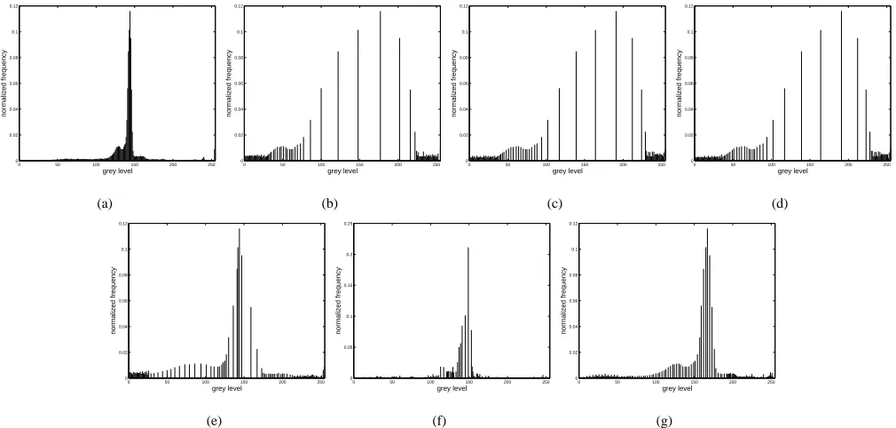
[image:15.612.61.558.51.171.2]0 50 100 150 200 250 0 0.02 0.04 0.06 0.08 0.1 0.12 grey level normalized frequency (g)
Fig. 8. Histograms of original and enhanced images shown Fig. 6: (a) original image; (b) GHE; (c) BPHEME; (d) FHSABP; (e) HMF; (f) CEBGA; and (g)
proposed.
is almost parallel to the no-change mapping. However, in the proposed algorithm, the dynamic range of the input image is
modelled with GMM, which makes it possible to model the intensity values of sparks and smoke differently. Input grey-level
values are assigned to output grey-level values according to their representative Gaussian components. The non-linear mapping
is designed to utilise the full dynamic range of the output image. Thus, the proposed algorithm improves the overall contrast
while preserving the details of the image.
The input image of an island in Fig. 4 [22] has average brightness value of 125. The results obtained by the different
algorithms are similar as verified by the similar mapping functions in Fig. 7(b). BPHEME and FHSABP behaves exactly the
same way as GHE when the average brightness value is 127.5 [13], [14]. Since the average brightness value of the input
image is very close to 127.5, BPHEME and FHSABP algorithms obtains the similar target histograms. The slight difference
of FHSABP from BPHEME is due to exact histogram specification used in FHSABP. The results of HMF and CEBGA are
also a match because both algorithms employ similar edge information. Where the sky and sea converge, GHE, BPHEME and
FHSABP provide a higher contrast than HMF and CEBGA. The proposed algorithm provides a contrast which is neither too
[image:15.612.55.560.226.467.2](a) (b) (c) (d)
[image:16.612.59.557.51.265.2](e) (f) (g)
Fig. 9. Contrast enhancement results for image Plane: (a) original image; (b) GHE; (c) BPHEME; (d) FHSABP; (e) HMF; (f) CEBGA; and (g) proposed.
The input image in Fig. 5 shows an aerial view of a junction in a city [23] with an average brightness value of 181 which
is too high for recognizing the different objects. GHE increases the overall contrast of the image significantly, but the image
looks darker as is verified by its mapping function in Fig. 7(c). The contrast improvements obtained by using BPHEME,
FHSABP, HMF and CEBGA are very slight. HMF fails to provide an improvement due to weak edge information. The
proposed algorithm, on the other hand, does not darken the image and produces sufficient contrast for the different objects to
be recognized.
The image Girl shown in Fig. 6 consists of challenging conditions for an enhancement algorithm: very bright and dark
objects, and average brightness value of 139 as can be verified from the histogram of the Girl image shown in Fig. 8(a). The
histogram reveals that most of the grey levels of the input image are accumulated around grey level 144. Meanwhile, there
are uniform grey level distributions on the left and right sides of the sharp peak in the middle. Because average brightness
value of the input image is near to 127.5, GHE, BPHEME, and FHSABP performs very similar. This can be verified from
the visual results, mapping functions shown Fig. 7(d), and histograms demonstrated in Fig. 8(b)-(d). As can be seen from
the histograms, the output histograms fail to achieve smooth distribution between high and low values of grey levels. Thus,
the enhancement results of GHE, BPHEME, and FHSABP are visually unpleasing. Meanwhile, the output histogram of HMF
achieves smoother distribution in between low and high grey values, thus HMF achieves more natural looking output as shown
in Fig. 8(e) when it is compared with that of GHE, BPHEME, and FHSABP. CEBGA produces natural looking output image,
however the overall enhancement is not significant. As can be seen from mapping function and histogram in Fig. 7(d) and
Fig. 8(f), CEBGA produces minor alterations on the input image. The result of the proposed algorithm is shown Fig. 6(g). The
proposed algorithm preserves the overall distribution shape, meanwhile it achieves to redistribute the grey levels of the input
image within the dynamic range without destroying natural look of the enhanced image. Although it slightly darkens the hair
of woman, still the overall natural look is not destroyed while the perceived contrast is improved significantly.
2) Colour Images: In Fig. 9, the over enhancement provided by GHE, BPHEME and FHSABP whitens some areas of the
concrete ground. HMF and CEBGA provide similar results where the slight contrast enhancement with respect to the input
image is apparent, whereas the proposed algorithm enhances the contrast and the average brightness to improve the overall
(a) (b) (c) (d)
[image:17.612.57.560.51.265.2](e) (f) (g)
Fig. 10. Contrast enhancement results for image Ruins: (a) original image; (b) GHE; (c) BPHEME; (d) FHSABP; (e) HMF; (f) CEBGA; and (g) proposed.
(a) (b) (c) (d)
(e) (f) (g)
Fig. 11. Contrast enhancement results for image Hats: (a) original image; (b) GHE; (c) BPHEME; (d) FHSABP; (e) HMF; (f) CEBGA; and (g) proposed.
proposed algorithm improve the overall contrast considerably and maintain high visual quality. In Fig. 11, GHE, BPHEME and
FHSABP result in loss of details in the clouds and on the top of the yellow hat, whereas HMF and CEBGA retain the details
while increasing the contrast. However, the contrast between the right side of the wall and the sky is not sufficiently high. The
proposed algorithm keeps the details while improving the overall contrast. Finally, in Fig. 12, GHE makes the stones around the
window and the pink flower very bright; hence, the enhanced image has an unnatural look. Although BPHEME and FHSABP
performs better than GHE, it still does not remove this effect completely. This effect is reduced by HMF, CEBGA and the
proposed algorithm. Also, the colours of window and wall are better differentiated in the result of the proposed algorithm.
Turgay: Please skip this paragraph as it needs new evaluation scores. In order to assign a visual assessment score to each
algorithm for each enhanced image, subjective perceived quality tests are performed by a group of ten subjects on the results
of the five algorithms for the eight test images. For each test on a test image, a subject is shown two images: the test image
[image:17.612.55.561.293.512.2](a) (b) (c) (d)
(e) (f) (g)
Fig. 12. Contrast enhancement results for image Window: (a) original image; (b) GHE; (c) BPHEME; (d) FHSABP; (e) HMF; (f) CEBGA; and (g) proposed.
TABLE II
AVERAGE OFSUBJECTIVEQUALITYTESTSCORES.
Image GHE FHSABP HMF CEBGA Prop.
Fireworks “Bad” “Bad” “Good” “Good” “Good”
Island “Bad” “Bad” “Good” “Good” “Good”
City “Good” “Bad” “Bad” “Bad” “Good”
Wolf “Bad” “Bad” “Bad” “Good” “Good”
Plane “Bad” “Bad” “Good” “Good” “Good”
Ruins “Bad” “Bad” “Bad” “Good” “Good”
Hats “Good” “Good” “Bad” “Good” “Good”
Window “Good” “Good” “Bad” “Bad” “Good”
by assigning a fuzzy score of “Bad” for weak enhancement, and “Good” for visually pleasing enhancement. The test on the
same input image is repeated for the processed images generated by the other four algorithms. For each processed image of
an algorithm, we average the scores from the ten subjects. In the averaging operation, when the number of “Good” scores are
higher than “Bad” scores, then the processed image is deemed as “Good”, and vice versa. The visual assessment scores as
shown in Table II validate our subjective evaluations that the proposed algorithm provides good visual quality enhancement.
B. Quantitative Assessment
The quantitative measures AMBE, DE, and EBCM may fail to provide enhancement measures which are parallel with
perceived image quality. For instance for Girl image, GHE, BPHEME, FHSABP, HMF, CEBGA, and proposed method produces
AMBE values of 5.60, 5.50, 5.50, 10.30, 1.60, and 12.90, respectively. CEBGA achieves the best in terms of brightness
preservation where the proposed method performs the worst. The Girl image has DE value of 3.87, meanwhile GHE, BPHEME,
FHSABP, HMF, CEBGA, and proposed method produces DE values of 3.65, 3.65, 3.65, 3.70, 3.45, and 3.81, respectively.
The proposed method achieves the best DE value. The Girl image has very low contrast measure EBCM value of 0.08. GHE,
BPHEME, FHSABP, HMF, CEBGA, and proposed method results in EBCM values of 0.23, 0.22, 0.22, 0.17, 0.11, and 0.12. All
methods achieve to produce higher values of EBCM with respect to the EBCM value of original Girl image. GHE, BPHEME,
[image:18.612.185.421.321.450.2]100 200 300 50 100 150 200 index MB GHE
100 200 300 50 100 150 200 index MB BPHEME
100 200 300 50 100 150 200 index MB FHSABP
100 200 300 50 100 150 200 index MB HMF
100 200 300 50 100 150 200 index MB CEBGA
100 200 300 50 100 150 200 index MB Proposed (a)
100 200 300 3 3.5 4 4.5 5 5.5 image index DE GHE
100 200 300 3 3.5 4 4.5 5 5.5 image index DE BPHEME
100 200 300 3 3.5 4 4.5 5 5.5 image index DE FHSABP
100 200 300 3 3.5 4 4.5 5 5.5 image index DE HMF
100 200 300 3 3.5 4 4.5 5 5.5 image index DE CEBGA
100 200 300 3 3.5 4 4.5 5 5.5 image index DE Proposed (b)
100 200 300 0 0.1 0.2 0.3 0.4 0.5 image index EBCM GHE
100 200 300 0 0.1 0.2 0.3 0.4 0.5 image index EBCM BPHEME
100 200 300 0 0.1 0.2 0.3 0.4 0.5 image index EBCM FHSABP
100 200 300 0 0.1 0.2 0.3 0.4 0.5 image index EBCM HMF
100 200 300 0 0.1 0.2 0.3 0.4 0.5 image index EBCM CEBGA
[image:19.612.63.556.53.207.2]100 200 300 0 0.1 0.2 0.3 0.4 0.5 image index EBCM Proposed (c)
Fig. 13. Quantitative performance results on 300 images from Berkeley dataset [24]: (a) results for MB; (b) results for DE; and (c) results for EBCM. The
reference measurements from the original image is shown in red colour, meanwhile the measurements from the processed images resulted from different
algorithms are shown in black colour.
correlation between between EBCM and perceived contrast enhancement, it does not always mean that the higher value of
EBCM means better perceived contrast enhancement.
In order to test algorithms’ performance quantitatively in terms of brightness and entropy preservation as well as contrast
improvement, they are applied on 300 test images of Berkeley image dataset [24]. MB, DE, and EBCM values are computed
from original and processed images. In reported results, the measurement values from the original images are sorted in ascending
order and the images are indexed accordingly. The quantitative results for MB, DE, and EBCM are shown in Fig. 13(a), (b),
and (c), respectively.
The MB values in Fig. 13(a) show that except GHE all algorithms follow general trend in the mean brightness value,
i.e.when the mean brightness value of the original image is low so do the output image, and vice versa. GHE consistently
maps the mean brightness value of the output image very close to 127.5 which is the mid value of the 8-bit grey-level dynamic
range. The average of AMBE resulted from GHE over dataset is 21.09. Meanwhile, BPHEME and FHSABP achieves the best
brightness preservation as can be seen from the plots. Both algorithms produces very similar results for the whole dataset. This
is mainly due to the target histograms of BPHEME and FHSABP are similar to each other. The averages of AMBE resulted
from BPHEME and FHSABP over dataset are 1.30 and 1.28, respectively. On the average, the proposed method performs
better than HMF and HMF performs better than CEBGA in terms of brightness preservation. The averages of AMBE resulted
from HMF, CEBGA, and the proposed method are 10.07, 12.23, and 8.80, respectively.
GHE, BPHEME, and FHSABP performs very similar results in terms of DE on Berkeley dataset as shown Fig. 13(b). The
average absolute discrete entropy difference between the input and out images over dataset for GHE, BPHEME, and FHSABP
are 0.12, 0.12, and 0.11, respectively. Fig. 13(b) also shows that CEBGA performs the worst with the average absolute discrete
entropy difference of 0.38. Meanwhile, HMF and the proposed method achieves good performance in terms of entropy. The
average absolute discrete entropy difference between the input and out images over dataset for HMF and the proposed method
are 0.05, and 0.04, respectively. Since the entropy is related with the overall image content, one can say that for Berkeley
dataset the proposed method can preserve the overall content of the image while improving its contrast.
The EBCM measures are shown in Fig. 13(c). Although high EBCM does not always mean a good and natural image
enhancement, however it is, at least, expected that the output image’s EBCM value is higher than that of the input image. Out
(a) (b) (c)
Fig. 14. High dynamic range compression results. (a) Original image. Processed image obtained using: (b) [27]; and (c) proposed algorithm.
286, and 300 output images, respectively, which have higher than or equal to EBCM values with that of the input images.
Meanwhile, the average absolute EBCM difference between the input and out images over dataset for GHE, BPHEME, FHSABP,
HMF, CEBGA, and proposed method are 0.0652, 0.0603, 0.0573, 0.0361, 0.0278, and 0.0366, respectively. As expected, GHE
provides the highest contrast improvement in terms of EBCM. Meanwhile, BPHEME and FHSABP performs very similar and
slightly worse than GHE. BPHEME performs better than FHSABP, because of lowpass filtering employed in exact histogram
specification used in FHSABP. Meanwhile, the proposed method and HMF performs similar and CEBGA provides the worst
performance. It is worth to note that only two algorithms, BPHEME and the proposed method, achieves to make EBCM
improvement with respect to the input image.
C. Application to High Dynamic Range Compression
The proposed algorithm can be applied for rendering high dynamic range (HDR) images on conventional displays. Thus,
we compare some of our results with those of the state-of-the-art method proposed by Fattal et al. [27]. In the Fattal et al.
method, the gradient field of the luminance image is manipulated by attenuating the magnitudes of large gradients. A low
dynamic range image is then obtained by solving a Poisson equation on the modified gradient field. The results in [27], a few
of which are in Fig. 14, show that the method is capable of drastic dynamic range compression, while preserving fine details
and avoiding common artefacts such as halos, gradient reversals, or loss of local contrast. Fig. 14 also shows that the proposed
algorithm produces comparable results. It is worth noting that our results are obtained without any parameter tuning.
IV. CONCLUSIONS
In this paper, we proposed an automatic image enhancement algorithm which employs Gaussian mixture modelling of an
input image to perform non-linear data mapping for generating visually pleasing enhancement on different types of images.
Performance comparisons with state-of-the-art techniques show that the proposed algorithm can achieve good enough image
images without any parameter tuning. It can also be used to render high dynamic range images. It does not distract the overall
content of an input image with high enough contrast. It further improves the colour content, brightness and contrast of an
image automatically.
REFERENCES
[1] R. C. Gonzalez and R. E. Woods, Digital Image Processing, 3rd ed. Upper Saddle River, NJ, USA: Prentice-Hall, Inc., 2006.
[2] D. Jobson, Z. Rahman, and G. Woodell, “A multiscale retinex for bridging the gap between color images and the human observation of scenes,” IEEE
Trans. Image Process., vol. 6, no. 7, pp. 965–976, Jul 1997.
[3] J. Mukherjee and S. Mitra, “Enhancement of color images by scaling the dct coefficients,” IEEE Trans. Image Process., vol. 17, no. 10, pp. 1783–1794,
Oct 2008.
[4] S. Agaian, B. Silver, and K. Panetta, “Transform coefficient histogram-based image enhancement algorithms using contrast entropy,” IEEE Trans. Image
Process., vol. 16, no. 3, pp. 741–758, Mar 2007.
[5] R. Dale-Jones and T. Tjahjadi, “A study and modification of the local histogram equalization algorithm,” Pattern Recognit., vol. 26, no. 9, pp. 1373–1381,
September 1993.
[6] T. K. Kim, J. K. Paik, and B. S. Kang, “Contrast enhancement system using spatially adaptive histogram equalization with temporal filtering,” IEEE
Trans. Consumer Electron., vol. 44, no. 1, pp. 82–87, Feb 1998.
[7] C.-C. Sun, S.-J. Ruan, M.-C. Shie, and T.-W. Pai, “Dynamic contrast enhancement based on histogram specification,” IEEE Trans. Consumer Electron.,
vol. 51, no. 4, pp. 1300–1305, Nov 2005.
[8] Y.-T. Kim, “Contrast enhancement using brightness preserving bi-histogram equalization,” IEEE Trans. Consumer Electron., vol. 43, no. 1, pp. 1–8, Feb
1997.
[9] Y. Wang, Q. Chen, and B. Zhang, “Image enhancement based on equal area dualistic sub-image histogram equalization method,” IEEE Trans. Consumer
Electron., vol. 45, no. 1, pp. 68–75, Feb 1999.
[10] S.-D. Chen and A. Ramli, “Minimum mean brightness error bi-histogram equalization in contrast enhancement,” IEEE Trans. Consumer Electron.,
vol. 49, no. 4, pp. 1310–1319, Nov 2003.
[11] ——, “Contrast enhancement using recursive mean-separate histogram equalization for scalable brightness preservation,” IEEE Trans. Consumer Electron.,
vol. 49, no. 4, pp. 1301–1309, Nov 2003.
[12] M. Abdullah-Al-Wadud, M. Kabir, M. Dewan, and O. Chae, “A Dynamic Histogram Equalization for Image Contrast Enhancement,” IEEE Trans.
Consumer Electron., vol. 53, no. 2, pp. 593–600, May 2007.
[13] C. Wang and Z. Ye, “Brightness preserving histogram equalization with maximum entropy: a variational perspective,” IEEE Trans. Consumer Electron.,
vol. 51, no. 4, Nov 2005.
[14] C. Wang, J. Peng, and Z. Ye, “Flattest histogram specification with accurate brightness preservation,” IET Image Process., vol. 2, no. 5, pp. 249–262,
Oct 2008.
[15] T. Arici, S. Dikbas, and Y. Altunbasak, “A Histogram Modification Framework and Its Application for Image Contrast Enhancement,” IEEE Trans.
Image Process., vol. 18, no. 9, pp. 1921–1935, Sep 2009.
[16] S. Hashemi, S. Kiani, N. Noroozi, and M. E. Moghaddam, “An image contrast enhancement method based on genetic algorithm,” Pattern Recognit.
Lett., vol. 31, no. 13, pp. 1816–1824, 2010.
[17] D. Reynolds and R. Rose, “Robust text-independent speaker identification using gaussian mixture speaker models,” IEEE Trans. Speech Audio Process.,
vol. 3, no. 1, pp. 72–83, Jan 1995.
[18] R. O. Duda, P. E. Hart, and D. G. Stork, Pattern Classification, 2nd ed. Wiley-Interscience, Nov 2000.
[19] M. Figueiredo and A. Jain, “Unsupervised learning of finite mixture models,” IEEE Trans. Pattern Anal. Mach. Intell., vol. 24, no. 3, pp. 381–396, Mar
2002.
[20] M. Abramowitz and I. A. Stegun, Handbook of Mathematical Functions with Formulas, Graphs, and Mathematical Tables. New York: Dover Publications,
1965.
[21] Retrieved on Aug 2010 from the World Wide Web: http://www.imagecompression.info/test images/.
[22] Retrieved on Aug 2010 from the World Wide Web: http://r0k.us/graphics/kodak/.
[23] Retrieved on Aug 2010 from the World Wide Web: http://sipi.usc.edu/database/.
[24] D. Martin, C. Fowlkes, D. Tal, and J. Malik, “A database of human segmented natural images and its application to evaluating segmentation algorithms
and measuring ecological statistics,” in Proc. 8th Int. Conf. Comput. Vis., vol. 2, Jul 2001, pp. 416–423.
[26] A. Beghdadi and A. L. Negrate, “Contrast enhancement technique based on local detection of edges,” Comput. Vis. Graph. Image Process., vol. 46,
no. 2, pp. 162–174, 1989.
[27] R. Fattal, D. Lischinski, and M. Werman, “Gradient domain high dynamic range compression,” in Proc. 29th Annual Conf. Comput. Graph. Interactive


![Fig. 13.Quantitative performance results on 300 images from Berkeley dataset [24]: (a) results for MB; (b) results for DE; and (c) results for EBCM](https://thumb-us.123doks.com/thumbv2/123dok_us/9639109.466286/19.612.63.556.53.207/quantitative-performance-results-berkeley-dataset-results-results-results.webp)
![Fig. 14.High dynamic range compression results. (a) Original image. Processed image obtained using: (b) [27]; and (c) proposed algorithm.](https://thumb-us.123doks.com/thumbv2/123dok_us/9639109.466286/20.612.72.541.52.299/dynamic-compression-results-original-processed-obtained-proposed-algorithm.webp)
