Investigating a Zero One law for Linear Temporal Logic statements in large random graphs

BSc Thesis Applied Mathematics

Investigating a Zero-One Law

for Linear Temporal Logic

Statements in Large Random

Graphs

Carmen Tretmans

Supervisor: Prof. Dr. N. Litvak

January, 2019

Investigating a Zero-One Law for Linear Temporal Logic

Statements in Large Random Graphs

Carmen Tretmans∗

January, 2019

Abstract

This article investigates the existence of a Zero-One law for Linear Temporal Logic in random graphs. A sample statement, Always, formulated in Linear Temporal Logic is tested in four dierent regimes of directed as well as undirected random graphs. For two of the regimes, the ones with the highest edge probability, the probability of an Always statement to hold tends to zero when the number of nodes of the graph tends to innity. A Zero-One Law could not be disproved. For the remaining two regimes, when the graph has a tree-like structure, a counterexample of a Zero-One law is found for the undirected random graph. For the directed random graph a counterexample in this regime is assumed but not yet proven. In conclusion, a Zero-One law does not hold for Linear Temporal Logic in at least some regimes of random graphs.

Keywords: Binomial Random Graph, Linear Temporal Logic, Zero-One Law

1 Introduction

Linear Temporal Logic statements for graphs are widely used for model checking purposes [1]. It is used in model checking, when properties of a system, e.g. a software or a hardware system, needs to be expressed. If a property of these system needs to be checked, the system is modeled as a graph where a node is assigned to every state of the system. Properties are assigned to every node, for example one can assign a property `critical' or `non-critical' to every node, representing whether the corresponding state of the system is critical or non-critical. The property is tested on the graph. Linear Temporal Logic covers statements as `Always' and `Eventually'. For example, one wants to check whether a system fulls the statement `Eventually critical', to check whether the system can reach a `critical' state. Linear Temporal Logic formulae are mainly checked using algorithms on existing graphs. However, due to the so called state-explosion problem, it is hard to model large systems by deterministic graphs. To still get an idea about the behaviour of these large systems, one uses random graphs with a large number of nodes. The random graphs are build on a vertex set n. Every possible edge between every pair of vertices exists with a given

probabilityp(n). If one choses a random graph in the same regime, i.e. choose a matching

edge probability, as the system, the random grahp has the same behavior as the modeled system. The properties of these large random graphs can be an indication for the behavior of the large systems.

We know by [4, 9] that a Zero-One law for rst order logic holds. That is, for a graph with

a number of nodes tending to innity, the probability that a rst order logic statement holds will either tend to zero or to one. First order logic statements are of the form `Is the graph connected?' or `Is there a triangle in the graph?'. A more precise denition of the Zero-One law and rst order logic can be found in the remainder of this article. Of interest is whether Linear Temporal Logic, as described in [1], satises a Zero-One law as well. If this is the case, all Linear Temporal Logic statements will either occur almost surely or almost never in large random graphs and one could draw interesting conclusions for systems with a large number of states.

In this article we will not focus on an entire overview of Linear Temporal Logic and a Zero-One law for this logic and we do not try to prove a Zero-One law for Linear Temporal Logic in general. Instead, we will focus our attention on a specic example statement in Linear Temporal Logic, the Always statement. We will investigate whether the Always statement meets a Zero-One law in certain regimes of random graphs. Herewith, we hope to achieve some insight in the behaviour of Linear Temporal Logic statements in large random graphs and the existence of a possible Zero-One law.

Problem Description Consider a random graph with n vertices, where n tends to

innity. Between each of the vertices there exists an edge with probability0 < p(n) <1,

independently of other edges. Assign to each of the vertices in the graph a red label with probability0< q(n)<1or a blue label with probability1−q(n). What is the probability,

for a random vertex S, that all possible paths starting at S only contain red vertices?

That is, what is the probability of the vertex S satisfying Always Red when the number

of nodes,n, of the graph tends to innity? We will investigate the probability of Always

Red for four dierent edge probabilities in undirected as well directed random graphs. The four edge probabilities are:

• p(n) =c, where0< c <1,

• p(n) =clog(_nn), where0< c≤1,

• p(n) = λ_n where0< λ <1

• p(n) = λ_n whereλ >1.

In Section 2 we dene structures used in the article. In Section 3 we will state preliminary results regarding the Zero-One law for rst order logic, the behaviour of an undirected ran-dom graph varying its number of edges and some results on branching processes. Section 4 we will classify each of our edge probability regimes into dierent asymptotic behaviours. In Section 5 we determine the probability that the Always Red statement holds in the undirected random graph for all the edge probability regimes. In Section 6 we will give insight in the Always Red statement in directed random graphs.

2 Denitions

In this section we will give an overview of the formal denitions of the regularly used expressions in this article. We give the random graph denition described in [6].

Denition 2.1 (Binomial Undirected Random Graph). The binomial undirected random graph G(n, p) is constructed on the vertex set {1, ..., n}. Between every pair of vertices,

an undirected edge is included with probability p(n) ∈ (0,1) and no edge is included with

probability 1−p(n). The n₂ possible edges are placed independently. Note that in such

Denition 2.2 (Binomial Directed Random Graph). The binomial directed random graph

G(n, p) is constructed on the vertex set {1, ..., n}. Between every ordered pair of vertices,

a directed edge is included with probability p(n) ∈ (0,1) and no edge is included with

probability 1−p(n). Then(n−1) possible edges are placed independently. [6]

Given a random graph we can assign a degree value to each of the vertices.

Denition 2.3 (Vertex Degree). For an undirected graphs the degree of a vertex,v, denoted

by d(v), is the number of adjacent vertices of v. This number is equal to the number of

edges incident tov. For a directed graph one distinguishes between the in-degree of a vertex,

denoted bydin(v), and the out-degree of a vertex, denoted by dout(v). The in-degree equals

the number of ingoing edges, e.g. edges of the form w →v, where w is any other vertex.

The out-degree equals the number of edges of the form v → w, that is edges starting at

vertexv and ending at any other vertexw.

To every vertex of a graph labels can be assigned. We only consider the labels red and blue. The labels are assigned using random vertex colouring as denes as follows.

Denition 2.4 (Random Vertex Colouring). Consider a random graphG(n, p). We say,

G(n, p) is a coloured graph with colour probability q(n), if each vertex of G(n, p) receives a

red label with probabilityq(n)∈(0,1) and a blue label with probability1−q(n).

To check whether a system holds a given property, we have to consider all possible states that can be reached from a starting state. Corresponding to a graph, we have to consider all possible paths starting atS. A path is dened as follows.

Denition 2.5 (Path). A path starting at vertexv1is a sequence of states< v1, v2,· · ·vk>,

wherek may be innite, such that (vi, vi+1) is in the edge set for all1≤i≤k−1 . Aim of this article is to investigate whether a Zero-One law holds for Linear Temporal Logic. Linear Temporal Logic is dened in [1].

Denition 2.6 (Linear Temporal Logic). Linear Temporal Logic (LTL) is constructed from atomic propositions AP, Boolean connectors (conjunction and negation) and two basic temporal modalities, (pronounced `next') and ∪ (pronounced `until'). The statements

are build using the following grammar rules:

ϕ::=true | a | ϕ1∧ϕ2 | ϕ | ϕ1∪ϕ2

where a ∈ AP. A vertex S meets a statement ϕ, denoted by S ϕ, if all vertices in all

possible paths, starting at S, meet the statementϕ.

Statements in Linear Temporal Logic are of the form S ϕ, where S is a vertex of a

graph. For example, the statement S a holds if S has the property a. Thus S red

holds if the vertexS has the label red. The statement S ϕholds if the successors of S has the property ϕ. The statement S ϕ1 ∪ϕ2 holds if, starting in S, S and all it's successor states have the propertyϕ1 till the path has a vertex with property ϕ2. For a more detailed description of Linear Temporal Logic we refer the reader to [1, Chapter 5]. We will investigate the Linear Temporal Logic statement Always in dierent random graph regimes. The Always statement is dened in [1].

Denition 2.7 (Always). The Linear Temporal Logic statement `Always' is denoted by . The statement `S ϕ' holds ifS and all its successor states have the propertyϕ. The

property `S ϕ' fails if there is at least one vertex in a path starting at S that does not

have the property ϕ. Always ϕis satised if and only if it is not the case that (¬ϕ) holds

The Always Red statement for a vertex S thus describes the property that all possible

paths starting in S only pass through red vertices. The property fails if there exists a blue vertex in a path starting atS.

3 Background

In this section we will state some preliminary results content-covering the Zero-One law for rst order logic, the random graph regimes of the Erd®s-Rényi random graph and some useful theorems on branching processes. The Zero-One law for rst order logic is of interest since we try to investigate a Zero-One Law for Linear Temporal Logic. The random graph regimes of the Erd®s-Rényi random graph are our object of investigation, and branching properties help to approximate the structure of random graph in some regimes.

3.1 Zero-One Law

Fagin proved in [4] a Zero-One law for rst order logic statements for graphs, as in Theo-rem 3.1. Of interest is whether the Linear Temporal Logic satises a Zero-One law, too. First order logic is dened as in [8].

Denition 3.1 (First Order Logic for Graphs). The rst order logic for graphs is build up from atomic formulae of the formvi =vj and vi ∼vj. Here, vi denote the underlying

vertices of the graph. The two binary predicates, equality (=) and adjacency (∼), are

assumed to be symmetric. Furthermore, adjacency is assumed to be anti-reexive. A rst order logic statement may contain the logical connectives conjunction, disjunction, negation and implication (∧,∨,¬,→) and quantiers ( ∃,∀).

The Zero-One law for rst order logic is dened as follows.

Theorem 3.1 (Zero-One Law for First Order Logic statements for Graphs). LetG(n, p)

be a random graph with a number of verticesn and edge probability p ∈[0,1]. Let A be a

rst order logic statement for graphs. Then, for all xedp and statement A

lim

n→∞P(G(n, p) |= A) = 0or1 .

That is, every rst order sentence is either almost always true or almost always false for a random graph. In our set up, the Always Red statement dened in Section 2 cannot be expressed as a rst order logic statement. Indeed, we divide the vertices in two distinct sets, a set with red vertices and a set with blue vertices. Therefore, we need a higher order logic to describe the Always Red property. In conclusion, Theorem 3.1 does not apply to Linear Temporal Logic statement.

3.2 Evolution of the Erd®s-Rényi Random Graph

Erd®s and Rényi described the process of evolution of the uniform random graph [3]. The uniform random graph is given byG(n, M(n))wherenis the number of vertices andM(n)

is the number of edges of the graph. The random graph is chosen uniformly out of all pos-sible graphs withn vertices and M(n) edges. Erd®s and Rényi distinguished ve phases

through which the graph passes when M(n) grows from 1 to n₂, the maximum number

Phase I : M(n)∼o(n) ,

Phase II : M(n)∼c n˜ with0<˜c < 1₂ ,

Phase III : M(n)∼˜c nwithc˜≥ 1₂ ,

Phase IV : M(n)∼˜c nlognwithc˜≤ 1 2 ,

Phase V : M(n)∼(nlogn)ω(n) withω(n)→ ∞ .

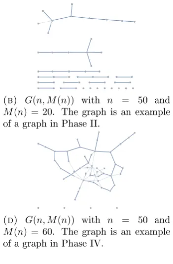
The graph changes throughout the phases from having mostly single isolated points in Phase I, to being completely connected in Phase V. We will describe the dierent Phases by explaining the behaviour of graphs in the dierent Phases and determining the average vertex degree,_d¯_{. Observe, that adding an edge to the graph increases the summed vertex}

degree of the graph, Pn

i=1d(vi), by two. We conclude Pni=1d(vi) = 2M(n). The average

vertex degree is given by _d¯ ₌ Pn i=1d(vi)

n =

2M(n)

n . In Figure 1 graphs in the dierent

regimes, i.e. in dierent Phases, are illustrated.

(a) G(n, M(n)) with n = 50 and

M(n) = 5. The graph is an example

of a graph in Phase I.

(b) G(n, M(n)) with n = 50 and

M(n) = 20. The graph is an example

of a graph in Phase II.

(c) G(n, M(n)) with n = 50 and

M(n) = 40. The graph is an example

of a graph in Phase III.

(d) G(n, M(n)) with n = 50 and

M(n) = 60. The graph is an example

of a graph in Phase IV.

(e) G(n, M(n)) with n = 50 and

M(n) = 1000. The graph is an example

of a graph in Phase V.

Figure 1: Randomly generated Uniform Random Graphs, G(n, M(n)), with

Phase I : A graph in Phase I is a graph with mostly isolated points. The average degree of a vertex tends to zero as the number of vertices tends to innity. All vertices with degree larger than zero are with probability tending to one in a tree. In Figure 1a a typical graph in Phase I is shown. Most of the vertices are isolated. The vertices having edges are in components containing just two vertices.

Phase II : In Phase II the graph contains trees and cycles. However, almost all vertices will be in components which are trees. The average degree of the vertices is equal to _d¯_{= 2˜c. Consequently, d}¯_{∈(0,1). Figure 1b displays a random graph in Phase II}

with ˜c= 0.4. Note, that isolated points can be seen as trees with a progeny of one.

The graph in Figure 1b therefore consist of only trees.

Phase III : WhenM(n)passes the threshold of Phase III the structure of the graph changes

abruptly. The trees present in Phase II merge to one giant component. The graph now contains one giant connected component with a complex structure and some small trees. The giant component will contain about G(˜c)n vertices where

G(˜c) = 1− 1

2˜c ∞

X

k=1

kk−1 k! (2˜ce

−2˜c₎k _.

The average degree of a vertex is equal to _d¯_{= 2c. Consequently, d}¯_{≥1. Figure 1c}

displays a random graph in Phase III with ˜c= 0.8. In Figure 1c one can distinguish

one connected component including cycles, one tree and some remaining isolated points.

Phase IV : A graph in Phase IV contains one giant connected component and some smaller components. The vertices which lie outside of the giant component are either isolated points or are in small trees. With probability tending to one, the graph consist of one giant connected component and some isolated points when the number of nodes of the graph tends to innity. The average degree of a vertex is equal to_d¯_{= 2˜clogn. In}

Figure 1d a graph in Phase IV withc˜= 0.3is displayed. One can clearly distinguish

one giant component and and some isolated points.

Phase V : WhenM(n) is in the range of Phase V, the entire graph is almost surely

con-nected. The average degree of a vertex equals _d¯_{= (2 logn)ω(n) and d}¯_{→ ∞when}

n → ∞. Figure 1e displays a graph in Phase V. The graph consists of one giant

component.

The results of this section are used in Section 4 to classify the binomial random graphs in dierent phases in order to determine their dierent behaviours. For a more detailed description of the phases and proof of results stated in the section, we refer the reader to [3].

3.3 Branching Process

As we will conclude later, in some regimes a random graph can be closely approximated by a Poisson branching process. We therefore will state some useful results on branching pro-cesses. The following section in mainly based on [10]. For an entire overview on branching processes we therefore refer the reader to [10, Chapter 3].

Consider a branching process where each individual has independent ospring with o-spring distribution X. The branching process will either die or survive innitely long.

byζ, whereζ = 1−η. The total progeny of the branching process is denoted byT.

The following results are used to understand the size of components in random graphs. For a random graph with an innite number of nodes it is, for example, of interest whether all vertices are part of one giant connected component or the graph is split up in dierent components. When comparing to a branching process, the graph will have just one giant component if the corresponding branching process survives almost surely. To determine the extinction probability of a branching process, we make use of Theorem 3.2.

Theorem 3.2 (Extinction Probability). The extinction probability η is the smallest

solu-tion in[0,1] of

η =GX(η) ,

withGX(s)being the probability generating function of the ospring densityX, i.e.,GX(s) =

E[sX].

Observe that ifE[X]<1thenη= 1. A branching process with expected ospring smaller

than on will die out almost surely. If E[X]>1then η <1. Prove of this results is given

in [10, Chapter 3]. I we want to compute the component size in a random graph, the total progeny of a branching process is of interest. Given a certain ospring distributionX, we

can determine the probability a branching process having a progeny ofn.

Theorem 3.3 (Law of Total Progeny). For a branching process with i.i.d. ospring dis-tribution X,

P(T =n) = 1

nP(X1+X2+. . .+Xn=n−1),

where(Xi)ni=1 are i.i.d. copies of X.

Proof of this results can be found in [10]. When it is known that a random graph consists of trees with a nite number of nodes we compare the random graph with a branching process based on extinction. The distributions (pk)k≥0 and (p0k)k≥0 are called conjugate pairs ifp0_k=ηk−1pk.

Theorem 3.4 (Duality principle for Branching Processes). Let (pk)k≥0 and (p0k)k≥0 be a conjugate pair of ospring distributions. The branching process with distribution (pk)k≥0 conditioned on extinction, has the same distribution as the branching process with ospring distribution(pk)0k≥0.

The proof of this Theorem and the denition of conjugate pairs can be found in [10]. As we will conclude later in this article, we can compare a random graph in some regimes to a Poisson branching process. We therefore will state some specic results for Poisson branching processes. IfX is Poisson distributed, the probability distribution of the total

progeny is given in Theorem 3.5.

Theorem 3.5 (Total Progeny for Poisson Branching Process). For a branching process with i.i.d. ospringX, where X has a Poisson distribution with mean λ,

Pλ(T =n) =

(λn)n−1

n! e

−λn _(n≥1).

Proof. By Theorem 3.3

Pλ(T =n) =

1

Since (Xi)ni+1 are independently Poisson distributed with mean λ the equation can be rewritten by

1

nP(X1+X2+. . .+Xn=n−1) =

1

nP( ˆX=n−1),

where_Xˆ _{is a Poisson distributed random variable with meannλ. Thus}

P(T =n) = 1

n

(nλ)n−1e−λn

(n−1)! =

(λn)n−1

n! e

−λn _(n≥1).

For a Possion branching process conditioned on extinction we formulate the following theorem.

Theorem 3.6 (Duality Principle for Poisson Branching Process). The branching process with Poisson distributed ospring with mean λ conditioned on extinction has the same

distribution as a branching process with Poisson ospring distribution with meanµ=ηλ.

Proof. Let pk be the ospring distribution of a Poisson branching process with mean λ.

Then the conjugate pair ofpk is given by

p0_k=ηk−1pk=ηke−λ(η−1)e−λ

λk k! =e

−λη(λη)k

k!

sincepk is Poisson distributed andη=eλ(η−1), obtained from Theorem 3.2. The ospring

distribution p0_k is again Poisson distributed with mean µ = ηλ. Applying Theorem 3.4

completes the prove.

4 Evolution of a Binomial Undirected Random Graph

To use the results of Erd®s and Rényi described in Section 3.2, we have to reformulate the ve phases to apply them to the binomial random graph model. Thus, instead of nding a threshold for the number of edges of the graphM(n), we try to nd a threshold for the edge

probability p(n). Since we consider large random graphs where n → ∞, we assume the

uniform random graphGu(n, M(n))to have the same behaviour as the binomial random

graphGb(n, p(n))withp(n) = M₍n(n) 2)

. Here, p(n)is equal to the ratio between the number

of edges in the graph and the total number of possible edges. Theorem 4.1, as stated in [5, p. 8-9], conrms this assumption.

Theorem 4.1 (Equivalence of Uniform Random Graph and Binomial Random Graph). Let Gb(n, p) be a binomial random graph and let Gu(n, M) be a uniform random graph.

Let 0≤p0≤1, s(n) =n

p

p(1−p)→ ∞ andω(n)→ ∞ arbitrarily slowly as n→ ∞.

(i) Suppose thatP is a graph property such thatP(Gu(n, M)∈ P)→p0 for all

m∈

n

2

p−ω(n)s(n),

n

2

p+ω(n)s(n)

.

Then P(Gb(n, p)∈ P)→p0 asn→ ∞.

(ii) Letp−=p−ω(n)s(n)/n3 andp+=p+ω(n)s(n)/n3. Suppose thatP is a monotone graph property such that P(Gb(n, p−)∈ P)→ ∞and P(Gb(n, p+)∈ P)→p0. Then

P(Gu(n, M)∈ P)→p0, asn→ ∞, where m=b n₂

Let property P be the property of a graph being in a given Phase. By Section 3.2,

P(Gu(n, M(n)) ∈ P) → 1 when n → ∞ whenever M(n) is in the corresponding range

of the Phase. If we letp(n) = M(n) (n

2)

, we can conclude from the rst part of Theorem 4.1 thatP(Gb(n, p(n))∈ P)→1 when n→ ∞. The binomial graph Gb(n, p(n))withp(n) = M(n)

(n 2)

is almost surely in the same Phase as the uniform random graph Gu(n, M(n)). By

rephrasing the thresholds for the dierent Phases using this result, we obtain: Phase I : p(n)∼o(n−1) ,

Phase II : p(n)∼ λ

n with0< λ <1 ,

Phase III : p(n)∼ λ_n withλ >1 ,

Phase IV : p(n)∼clog_nn withc≤1 ,

Phase V : p(n)∼ω(n)log_nn withω(n)→ ∞ .

We can classify each of the scaling regimes forp(n) in one of the phases.

p(n) =c with0< c <1: Let w(n) = c_logn_n. As n → ∞, w(n) → ∞. Now, p(n) can be

rewritten as p(n) =w(n)log_nn and thus the graph G(n, p) with p =c will be in the

regime of Phase V.

p(n) = clog_nn with0< c≤1: A graph G(n, p) withp(n) = clog_n n will be in Phase IV.

p(n) = λ_n with0< λ <1: The graph of G(n, p) withp= λ_n ,0< λ <1 will behave like a

graph of Phase II

p(n) = λ_n withλ >1: The graph of G(n, p) with p= λ_n,λ >1 will behave like a graph of

Phase III.

Using this results and the phases described in [3], a graph G(n, p) with p = c will be

almost surely connected and will consist of one giant component. A graph G(n, p) with

p(n) = clog_nn and c ≤ 1 contains one giant component and a few isolated points. For a

graphG(n, p) with p = λ_n and 0 < λ < 1, almost all vertices will be part of components

which are trees. If λ >1 the structure of the graph changes abruptly. There will be one

giant component and some small trees. The giant component will contain about G(λ)n

vertices where

G(λ) = 1− 1

λ ∞

X

k=1

kk−1 k! (λe

−λ₎k _{. (1)}

Consequently, the fraction of vertices lying in the giant component will be equal toG(λ).

The other vertices will lie in small trees.

5 Probability of Always Red in Undirected Random Graph

is the probability that all possible paths starting atS will contain only red vertices when

equals zero or one in all cases, we cannot draw any conclusions about a Zero-One law. If, however, the probability is strictly bounded by zero and one, a counterexample of a Zero-One law for Linear Temporal Logic is found. We know that a random graph passes through dierent phases as one increases the edge probability. We therefore believe that the Always Red statement occurs with dierent probabilities in dierent random graph regimes. We will compute the probability of Always Red for dierent edge probabilities. We will use the results of Section 4 to determine the behaviour of a random graph in the dierent regimes. We will start with thep(n) =ccase, followed by thep(n) = clog(_nn) and

p(n) = λ_n, 0 < λ < 1 and λ > 1 cases. For the p(n) =c and the p(n) = clog(_nn) case we

will nd analytical results of the Always Red property. For thep(n) = λ_n with0 < λ <1

and λ > 1 regimes we will nd bounds for the Always Red probability as well compute

numerical results. The Always Red statement is dened as in Denition 2.7. The vertex colouring is dened as in Denition 2.4, whereq(n)is the probability of a vertex being red.

LetS denote the starting vertex, chosen at random.

5.1 Always Red in coloured undirected random graph G(n, p)

with p(n) = c, 0 < c < 1

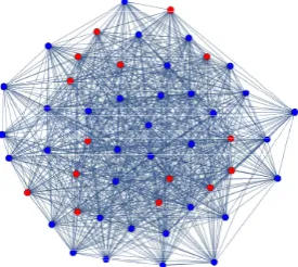
A random graph with edge probability p(n) = c is almost surely connected. A typical

graph with colour probabilityq= 0.3 can be found in Figure 2. From any starting vertex

S all other vertices can be reached. Since the property Always Red fails if we can nd a

path with just one blue vertex, all vertices of the graph have to be red for the property to hold. Since we consider graphs with an innite number of nodes, the probability of having only red vertices will tend to zero. We expect the probability of Always Red to tend to zero. This corresponds to the results found in Theorem 5.1.

Figure 2: Coloured Binomial Undirected Random Graph G(n, p) with n = 50,

p= 0.7 and colour probability q= 0.3. The Graph is an example of an undirected

random graph with edge probabilityp=c,0< c <1.

Theorem 5.1 (Always Red in coloured undirected random graphG(n, p) withp(n) =c).

For a coloured undirected random graph,G(n, p), with colour probabilityq∈(0,1)and edge

probability p(n) =c, c∈(0,1),

P(S red) = 0 when n→ ∞ .

Proof. The graph G(n, p) is connected with high probability, as described in Section 4.

That is

P(G(n, p) is conncected) = 1 for n→ ∞

By conditioning onG(n, p) being connected

P(S red) =P(S red|G(n, p) is conncected)P(G(n, p) is conncected )

+P(S red|G(n, p) is not conncected)P(G(n, p) is not conncected) =P(S red|G(n, p) is conncected) for n→ ∞ .

IfG(n, p) is connected, all states can be reached from a starting vertex S. Thus, if there

is at least one blue state we can nd a path for which the Always Red property does not hold. The property only holds if there are only red vertices. So

P(S red|G(n, p) is conncected) =P(∀ v:v is red) =qn

which converges to zero asntends to innity, since q <1. Concluding,

P(S red) = 0 for n→ ∞ .

5.2 Always Red in coloured undirected random graph G(n, p)

with p(n) = clog_nn, 0 < c ≤ 1

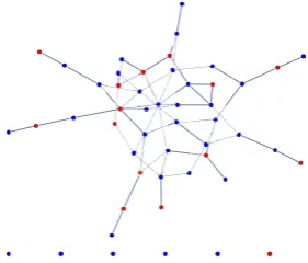
Whenp=clog_nn with0< c≤1, the graph consist of one giant connected component and

some isolated points. A typical graph in this regime with colour probabilityq = 0.3can be

found in Figure 3. IfS lies in the giant connected component, we expect a equal behaviour

of the Always Red statement as in thep(n) =cedge probability regime. If Sis an isolated

point, the probability of the Always Red property to hold is equal the colour probability

q. Either, S itself is red, in which case the property holds, or S is blue, in which case the

property fails. Of interest is with what probabilityS is an isolated point. For the Always

Red property is this regime we state Theorem 5.2.

Figure 3: Coloured Binomial Undirected Random Graph G(n, p) with n = 50,

p= 0.05and colour probabilityq= 0.3. The Graph is an example of an undirected

random graph with edge probabilityp=clog(_nn) with0< c <1.

Theorem 5.2 (Always Red in coloured undirected random graphG(n, p)withp(n) = clog_n n).

For a coloured undirected random graph,G(n, p), with colour probabilityq∈(0,1)and edge

probability p(n) =clog_nn, 0< c≤1,

Proof. The graph is with probability tending to one a graph with one giant component and some isolated points. Thus,S lies either in the giant component, denoted by Cmax, or

is an isolated point. By conditioning onS lying in the giant component

P(S red) =P(S red|S ∈ Cmax)P(S ∈ Cmax)

+P(S red|S 6∈ C_max)P(S 6∈ C_max) .

The vertex S is an isolated point if d(S) = 0. Since the vertex degree of S is binomial

distributed with d(S) ∼ Bin(n−1, p(n)), the probability of S being an isolated vertex

decreases with the number of vertices. IndeedP(d(S) = 0) = (1−clog_nn)n andP(d(S) = 0)→0 asn→ ∞. We therefore claim that the number of isolated points will be of order

O(1) when n→ ∞. The number of vertices in the giant component is of order n−O(1).

We can conclude

P(S∈ Cmax) =

n−O(1)

n = 1 ,

P(S6∈ C_max) = O(1)

n = 0

whenntends to innity. Furthermore, if S lies in the giant component, all vertices in the

giant component have to be red for the Always Red statement to hold. IfS is an isolated

point, onlyS needs to be red for the statement to hold. We conclude,

P(S red|S∈ Cmax) =qn−O(1) ,

P(S red|S6∈ Cmax) =q .

Thus,

P(S red) =qn−O(1) = 0for n→ ∞ .

5.3 Always Red in coloured undirected random graph G(n, p)

with p = λ_n,0 < λ <1

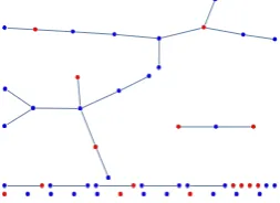
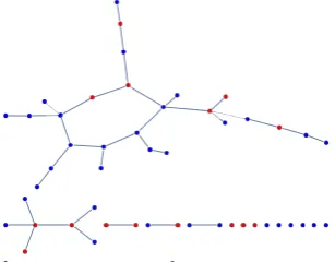
A graph with edge probability p(n) = λ_n, 0 < λ < 1, contains components which are

trees. See Figure 4 for a random graph in this regime. In this graph regime we expect the probability of the Always Red property to dier signicant from the previous described random graph regimes. The random graph contains no giant component. Furthermore, we expect all components to have a nite number of vertices, even though the total number of vertices will tend to innity. The probability of all vertices in the component of S are

red, and the Always Red property holds, will therefore be greater than zero.

Figure 4: Coloured Binomial Undirected Random Graph G(n, p) with n = 50,

p= 0.015and colour probabilityq = 0.3. The Graph is an example of an undirected

We will calculate the probability that all the vertices in the component ofS are red. Note

that the set of reachable vertices fromS and the set of vertices in the component ofS are

equivalent. LetC(S) denote the component ofS. Then,

P(S red) =P(∀ v∈ C(S) :v isred).

We will calculate the above probability by conditioning on the component size ofS, denoted

by |C(S)|. The components size can vary from 1, in case S is an isolated point, to n, in

case the whole graph is connected.

P(S red) =

n

X

i=1

P(∀ v∈ C(S) :v is red| |C(S)|=i) P(|C(S)|=i). (2)

Clearly,P(∀v∈ C(S) :vis red| |C(S)|=i) =qi. To calculate the component size|C(S)|,

we approximate the random graph by a branching process, since the graph will look like a collection of trees with high probability. Every vertex has with probabilityp(n) = λ_n an

edge to each of the other n−1 vertices. Thus, the degree of every vertex vi is binomial

distributed with

d(vi)∼Bin(n−1, p) .

Since the binomial distribution can be approximated by the Poisson distribution when n

tends to innity, we say that the degree of every vertex is distributed in the limit by

d(vi)∼P oi(λ) .

SinceSlies in a tree, we claim that the probabilityP(|C(S)|=i)is equal to the probability

of a branching process with Poisson ospring distribution with meanλhas a progeny ofi.

Thus, by using the results form section 3.3, Theorem 3.3,

P(|C(S)|=i) = (λi)

i−1

i! e

−λi _{(i≥1) .}

The total probability, as given in equation (2), equals

P(S red) =

n

X

i=1

qi(λi)

i−1

i! e

−λi

=

n

X

i=1

ii−1 i!

1

λ(λq)

i_e−λi _{. (3)}

Equation (3) gives the probability for the limiting object. We will continue by giving a sim-pler approximation for this equation to gain more insight in it's value and it's dependency onλandq. To approximate equation (3) we use Stirling's inequality given in Lemma 5.3.

We obtained Lemma 5.3 by simplifying the error bounds given in [7].

Lemma 5.3 (Stirlings Inequality). Forn∈_N\ {0}, Stirling's inequality is given by √

2πnn+12e−n≤n!≤nn+ 1

2e−n+1 . (4)

Proof. By the error bounds given in [7] we know

n! =√2πnn+12e−n·ern , where 1

It remains to prove that

1< ern _{< √}e

2π ⇐⇒ 0< rn<1−log(

√

2π) ,

by monotonicity of the exponential function. Clearly, rn > 0 for all n, wherefore the

correctness of the lower bound is proven. For the upper bound observe that the maximum value ofrnis given at n= 1, and thus,

rn< r1=

1

12 <1−log(

√

2π) ,

which proves the upper bound.

By substituting the results of Lemma 5.3 into equation (3) we can bound the probability by

n

X

i=1

ii−1 ii+12e−i+1

1

λ(λq)

i_e−λi_{≤P(S red)≤} n

X

i=1

ii−1

√

2πii+12e−i

1

λ(λq)

i_e−λi _.

This can be rewritten as

1

eλ

n

X

i=1

e−Iλ,q·i

i32

≤P(S red)≤ √1

2πλ

n

X

i=1

e−Iλ,q·i

i32

, (5)

where we dene the variableIλ,q by Iλ,q =λ−1−log(λq). Observe that Iλ,q is positive

for all0 < q < 1 and λ > 0. The summation in equation (5) for n → ∞ is equal to the

polygarithm function

Lis(z) =

∞

X

i=1

zi is ,

where z = e−Iλ,q and _{s =} 3

2. According to [2] the polygarithm function has a integral representation of

Lis(z) =

z

Γ(s)

Z ∞

0

ts−1

et_−zdt (6)

for allz, except z lying on the segment of the real axis from 1 to ∞. Since, in our case,

z=e−Iλ,q is bounded by zero and one,_{0< e}−Iλ,q _<1, the integral representation is valid and the summation equals

Li3 2(e

−Iλ,q_{) =} e

−Iλ,q

Γ(1.5)

Z ∞

0

t0.5

et_−e−Iλ,qdt . (7)

Here,Γ(s) is the Gamma-function withΓ(1.5) =

√

π

2 . With equation (5), equation (7) and

Iλ,q=λ−1−log(λq) we can formulate following Lemma:

Lemma 5.4 (Always Red in coloured undirected random graph G(n, p) with p(n) = λ_n, 0 < λ < 1). For a coloured undirected random graph, G(n, p), with colour probability

q∈(0,1) and edge probabilityp(n) = _nλ, 0< λ <1, 2q √ πe −λ Z ∞ 0 √ t

et_−λqe1−λdt≤P(S red)≤

2q

√

2πe

1−λ

Z ∞

0

√

t

et_−λqe1−λdt . (8)

Observe that the upper and lower bound only dier by a factor of k = √e

2π ≈ 1.0844,

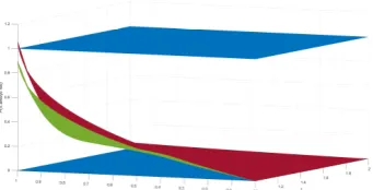
Numerical Solution of Equation (8) To solve equation (8) numerically, we use Mat-lab's implemented integral function. Graphs of the numerical results of equation (8) can be found below. The zero and one bounds are displayed blue. The Lower bound is displayed green, the upper bound is displayed red.

Figure 5: Numercial Results forP(S red)in the coloured undirected random

graph, G(n, p), withp= λ_n for 0< λ <1. The Zero and One bounds are displayed

blue. The lower bound is displayed green, the upper bound is displayed red.

The probability is increasing withq. As one can conclude from the numerical data, both,

upper and lower bound are larger than zero for all values of q and λ. The lower bound

does not exceed one. The upper bound, however, exceeds one for large values ofq.

Analytical Solution of Solving Equation (8) We will bound the integral of equa-tion (8), R∞

0

√

t

et_−e−Iλ,qdt, where Iλ,q = λ−1−log(λ, q). To estimate the integral we use Taylor expansion on 1

et_−e−λ,q. For convenience letx=et. Observe that x >1. Then,

1

x−e−Iλ,q =

1

x

1

(1−e−Iλ,q x ) = 1 x ∞ X j=0

e−jIλ,q

xj (9)

since0< e−Iλ,q_x <1. For the lower bound observe that

1

x ∞

X

j=0

e−jIλ,q

xj =

1

x(1 + e−Iλ,q

x +

e−2Iλ,q

x2 · · ·)>

1

x

since all terms of the sum are positive. We will estimate the lower bound of the integral by

Z ∞

0

√

t

et_−e−Iλ,qdt > Z ∞

0

√

t

etdt . (10)

For the upper bound observe that the tail of the sum of equation 9 consist of smaller order terms, since e−Iλ,q

x <1. Moreover, ( e−Iλ,q

x + e−2Iλ,q

x2 +e

−3_Iλ,q

x3 +· · ·) obtains its maximum for a minimum value of x. By substituting x= 1, the minimum value of et in t∈(0,∞),

we obtain

e−Iλ,q _+e−2Iλ,q_+e−3Iλ,q _{+· · ·=e}−Iλ,q_{(1 +e}−2Iλ,q_+e−3Iλ,q _{+· · ·) =e}−Iλ,q₍ 1

1−e−Iλ,q) since0< e−Iλ,q _<1. Therefore,

1

x−e−Iλ,q <

1

x(1 +

e−Iλ,q

1−e−Iλ,q) =

1

x

1

We will estimate the upper bound of the integral by

Z ∞

0

√

t

et_−e−Iλ,qdt <

1 (1−e−Iλ,q₎

Z ∞

0

√

t

et dt . (11)

By substituting this bounds in inequality (8) and solving the integralR∞

− √

t

et, we obtain

2

√

π

1

eλe −Iλ,q

Z ∞

0

√

t

et dt≤P(S red)≤

√

2

π

1

λe

−Iλ,q 1

(1−e−Iλ,q₎ Z ∞

0

√

t et dt ,

e−Iλ,q

eλ ≤P(S red)≤

1 √ 2π 1 λ 1

(eIλ,q −₁₎ . By substitutingIλ,q=λ−1−log(λq) we obtain

q

eλ < P(S red)<

1

√

2π q

eλ−1_−λq .

First observe that the lower bound ofP(S red) is larger than zero for allλ > 0 and

q > 0. However, for particular values of λ, it is possible for the upper bound to exceed

one. The upper bound forP(S red) is smaller than one whenever

1

√

2π

1

eIλ,q_λ−λ <1 ⇐⇒ 0< e

λ_{−eqλ−√}eq

2π .

Now let

fq(λ) =eλ−eqλ−

eq

√

2π .

From the rst and second derivative of fq(λ) we can conclude that fq(λ) has a local

minimum atλ= log(eq). From the denition offq(λ) we can conclude that

fq(log(eq)) =eq(1−log(eq)−

1

√

2π)

which is larger than zero whenever e−

1

√

2π ≈_{0.67 < q} . Whenever the local minimum of

fq(λ) is greater than zero,fq(λ) is greater than zero for all values of0< λ <1. Thus,

0< eλ−eqλ−√eq

2π whenevere −_√1

2π < q .

We can conclude that

1

eλ < P(S red)<

1

√

2π q

eλ−1_−λq for 0< λ <1 . (12)

Furthermore

0< P(S red)<1 for 0< λ <1 and e−

1

√

2π _{< q .} (13)

Observe that these results correspond to the numerical results found in Figure 5 since the lower bound is always greater than zero and the upper bound only exceeds one for large values ofq.

Theorem 5.5 (Always Red in coloured undirected random graph with p(n) = λ_n with 0< λ <1). For a coloured undirected random graphG(n, p) with edge probabilityp(n) = λ_n

with 0< λ <1 and colour probability q∈(0,1),

1

eλ < P(S red)<

1

√

2π q

eλ−1_−λq whenn→ ∞ .

Moreover,0< P(S red)for all values ofq, and 0< P(S red)<1for e−

1

√

2π < q. Theorem 5.5 is a powerful result in investigating a possible the Zero-One law. Theorem 5.5 contradicts a possible Zero-One law for at least some values ofλand q. Moreover, as, we

can conclude from the numerical results presented earlier this section, the Zero-One law does not hold for almost all values ofqandλsince the probability ofP(S red)is strictly

bounded by zero and one. Only for large values ofq we cannot draw any conclusions.

5.4 Always Red in coloured undirected random graph G(n, p)

with p = λ_n, λ > 1

When p(n) = λ_n with λ > 1, a random graph G(n, p) consists almost surely of one giant

component and some small trees. Figure 6 shows a typical graph in this regime. For the probability of Always Red we assume to nd similar results as for 0 < λ < 1 values

whenever S is in one of the trees. When S is in the giant component, we expect the

probability of Always Red to occur to tend to zero when the number of nodes tend to innity since the number of nodes in the giant component will tend to innity too.

Figure 6: Coloured Binomial Undirected Random Graph G(n, p) with n = 50,

p= 0.03and colour probabilityq= 0.3. The Graph is an example of an undirected

random graph with edge probabilityp= λ_n,λ= 1.5.

For λ > 1, the starting vertex S lies either in one giant connected component or in a

small tree. We will calculateP(S red) by conditioning on whetherS lies in the giant

component or not. LetC_max denote the giant component. Then,

P(S red) =P(S red|S ∈ Cmax) P(S∈ Cmax)

+P(S red|S 6∈ C_max) P(S6∈ C_max) .

Whenever S lies in the giant component the statement (S red) will only hold if all

vertices in the giant component are red. As described in Section 4, we know that the number of vertices in the giant component equalsG(λ)n, whereG(λ)is given in equation (1). The

the number of vertices of the graph tends to innity. The probability of all vertices in the giant component being red, will tend, as in thep(n) =ccase, to zero asn→ ∞. Thus

P(S red) =P(S red|S6∈ Cmax) P(S 6∈ Cmax) . (14)

For the probabilityP(S 6∈ Cmax)we state the following lemma:

Lemma 5.6 (Vertices outside of the Giant Component in an Undirected Random Graph

G(n, p)withp(n) = λ_n andλ >1). Given an undirected random graphG(n, p) withp(n) =

λ

n andλ >1wheren→ ∞. The probability for a vertex,v, chosen at random, to be outside

of the giant component is bounded by

2e−λ

√

π

Z ∞

0

t0.5

et_−λe1−λ ≤P(v6∈ Cmax)≤

√

2e1−λ π

Z ∞

0

t0.5

et_−λe1−λ . (15)

Proof. By [3] we know that the fraction of vertices inside of the giant component equals

G(λ) = 1− 1

λ ∞

X

k=1

kk−1

k! (λe

−λ₎k _,

and accordingly, the fraction of vertices outside of the giant component equals

P(S6∈ Cmax) =

1

λ ∞

X

k=1

kk−1 k! (λe

−λ₎k _{. (16)}

Using Stirling's inequality stated in Lemma 5.3, we can rewrite equation (16) by

1

eλ ∞

X

k=1

(λe1−λ)k

k32

≤P(v6∈ Cmax)≤

1 √ 2πλ ∞ X k=1

(λe1−λ)k

k32

.

We will make use of the integral representation of the poligarithm function Lis(z) =

P∞

i=1 z i

is given in equation (6) fors= 3₂ and z=λe1−λ. The integral representation of the polygarithm function is valid sinceλe1−λ<1. By substituting the integral representation

of the polygarithm function, we obtain the required result:

2e−λ

√

π

Z ∞

0

t0.5

et_−λe1−λ ≤P(v6∈ Cmax)≤

√

2e1−λ π

Z ∞

0

t0.5 et_−λe1−λ .

When S is outside of the giant component, the component ofS can be represented by a

branching process with mean ospring λ conditioned on extinction. With Theorem 3.4,

this equals a branching process with mean ospring µ = λη , where η is the extinction

probability of a branching process with mean ospring λ. Observe that 0 < µ < 1 and

a branching process with Poisson ospring distributionµ is described in Section 5.3. By

Theorem 5.5 2q √ πe −ηλ Z ∞ 0 √ t

et_−ηλqe1−ηλdt≤P(S red|S6∈ Cmax)

≤ √2q

2πe

1−ηλ

Z ∞

0

√

t

To compute the probabilityP(S red), we substitute equation (17) and the result of

Lemma 5.6 into equation (14) and obtain

(√2q

πe −ηλ Z ∞ 0 √ t

et_−ηλqe1−ηλdt)(

2e−λ

√

π

Z ∞

0

t0.5

et_−λe1−λdt)≤P(S red)

≤(√2q

2πe

1−ηλ

Z ∞

0

√

t

et_−ηλqe1−ηλdt)(

√

2e1−λ π

Z ∞

0

t0.5 et_−λe1−λdt)

By simplifying aboves equation we can state follwoing Lemma:

Lemma 5.7 (Always Red in coloured undirected random graph G(n, p) with p(n) = λ_n,

λ >1). For a coloured undirected random graph, G(n, p), with colour probabilityq ∈(0,1)

and edge probabilityp(n) = _nλ, λ >1,

4qe−λ−ηλ

π (

Z ∞

0

t0.5

et_−λe1−λdt)(

Z ∞

0

t0.5

et_−ηλqe1−ηλdt)≤P(S red)

≤ 2qe

2−λ−ηλ

π2 (

Z ∞

0

t0.5

et_−ηλqe1−ηλdt)(

Z ∞

0

t0.5

et_−λe1−λdt) as n→ ∞ .

Here,η is the extinction probability of a Poisson Branching Process with mean ospringλ.

To ndη, the extinction probability of a branching process with mean ospring λ, we use

the relation given in Theorem 3.2.

η =GX(η) , (18)

whereGX(s) is the probability generating function of the ospring distribution X. Since

the ospring distribution is a Poisson distribution with parameter λ, η is given by the

smallest solution of

η =eλ(η−1) .

We will obtain numerical results of the inequality in Lemma 5.7. To ndηwe will determine

the roots of

f(x) =eλ(x−1)−x

in the interval(0,1)numerically, using Matlab's fzero function. The integrals are

deter-mined numerically using Matlab's integral function. Plots of the numerical results can be found in Figure 7. The zero and one bound are displayed blue, the upper bound red and the lower bound green. Whenλincreases, the probability approaches zero, but never

reaches zero. This seems logical since the large connected component will grow when λ

increases and the probability ofS lying in the connected component will grow. If S lies in

the connected component, the probability of Always Red will tend to zero when the num-ber of states tend to innity, since the probability of a reachable blue state will increase to one. For smallλand large q the probability of always red tends to one, where the upper

bound exceeds one. For large λ the probability decreases with q. When λ is small, the

probability of S lying in a small component grows. When S lies in a small component

with nite reachable states, it is clear that the probability of always red increases with the probability of a state being red. In conclusion, P(S red) with p= λ_n, λ >1 does not

obey the Zero-One law for almost all values ofλandq. Forλclose to one and largeq we

Figure 7: Numercial Results forP(S red)in the coloured undirected random

graph, G(n, p), with p = λ_n, λ >1. The Zero and One bounds are displayed blue.

The lower bound is displayed green, the upper bound is displayed red.

As a result of the numerical results found in this section we will state the following theorem. Theorem 5.8 (Always Red in coloured undirected random graph withp(n) = λ_n,λ >1).

For a coloured undirected random graph G(n, p) with edge probability p(n) = λ_n,λ >1 and

colour probability q∈(0,1), there exists values for λand q, such that P(S red)6= 0 and

P(S red)6= 1 as n→ ∞ .

The theorem states that there exist values ofλandq that refute a possible Zero-One law.

6 Probability of Always Red in Directed Random Graph

colour probabilityq(n), as described in Dention 2.2. The probability of the Always Red

statement will be computed for dierent types of edge probabilities. The dierence with the previous section is the directedness of the random graph. We know that a random graph passes through dierent phases as one increases the edge probability. We therefore will consider dierent edge probabilities to determine the Always Red statement. Again, we will start with the p(n) = c edge probability case, followed by the p(n) = log(_nn) and

p(n) = cλ_n for 0 < λ <1 and λ > 1 cases. For the p(n) = c case we will nd analytical

results of the Always Red property. Thep(n) = log(_nn),p(n) = cλ_n with0< λ < and λ >1

cases will need further investigation since we were not able to nd any specic results in this article. However, we will try to give insight these regimes and formulate conjectures about the probability of the Always Red statement.

6.1 Always Red in coloured directed random graph G(n, p)

with p(n) = c, 0 < c < 1

To get a better understanding of a directed random graph in this regime we will rst state a theorem about strong connectivity in directed random graphs as stated in [6].

Theorem 6.1 (Strong Connectivity in Directed Binomial Random Graphs). Given a bi-nomial random graph G(n, p). For any xed c ∈ _R, if p = p(n) is a function of n, then

ˆ

p= log_nn+c is a threshold for strong connectivity.

The proof of this theorem can be found in [6]. The theorem states that

lim

n→∞P(G(n, p) is strongly connected) =

(

By Theorem 6.1, a directed random graph G(n, p) with p(n) = c is strongly connected.

Since we then, again, consider a giant connected component, we assume the Always Red statement to occur almost never. Figure 8 shows a typical graph in this regime.

Figure 8: Coloured Binomial Directed Random Graph G(n, p) with n = 50,

p = 0.7 and colour probability q = 0.3. The Graph is an example of a directed

random graph with edge probabilityp=c.

For the Always Red property in thep(n) =cregime, we will prove the following theorem.

Theorem 6.2 (Always Red in coloured directed random graph G(n, p) with p(n) = c).

For a coloured directed random graph,G(n, p), with colour probability q ∈(0,1)and edge

probability p(n) =c, c∈(0,1),

P(S red) = 0 when n→ ∞ .

Proof. With Theorem 6.1, we can conclude that a directed graph withp(n) =cis strongly

connected with high probability. That means, all vertices can be reached from a starting vertexS and the Always Red property does only hold if there are only red states.

P(S red) =P(∀v:v is red) =qn

which tends to zero asntends to innity, since q < 1.

6.2 Always Red in coloured directed random graph G(n, p)

with p(n) = clog(_nn), 0 < c ≤ 1

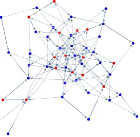
Figure 9: Coloured Binomial Directed Random Graph G(n, p) with n = 50,

p = 0.05 and colour probability q = 0.3. The Graph is an example of a directed

As one can see in Figure 9, the graph in the regime of p = clog(_nn) consists of one giant,

weakly connected component. However, some of the vertices have only outgoing edges and cannot be reached from any other vertex. Consider this vertices to be isolated vertices. then, the graph consists, as in the undirected case, of some isolated vertices and one giant component.

Since p(n) = clog(_nn) is in the regime of the threshold given in Theorem 6.1, we cannot

conclude whether the graph G(n, p) is strongly connected or not. Neither can we make

statements about strong connectivity in the giant component. We can only conclude that the the giant connected component is weakly connected. However, by Section 3.2, we know that the average degree of a vertex is given by_d¯_{=clogn. Thus, the average in-degree, as}

well the average out-degree grows with the number of nodes. Since this number grows, we expect the number of reachable vertices, from a starting vertexS in the giant component,

to tend to innity when the number of nodes of the graph tends to innity. We formulate this assumption in the following conjecture.

Conjecture 6.3 (Number of reachable vertices in a directed random graphG(n, p) with

p(n) =clog(_nn)). Given a directed random graph,G(n, p)with edge probabilityp(n) =clog(_nn),

0 < c ≤ 1. Let the giant component be the set of all vertices with at least one incoming

edge. The number of reachable vertices from any starting vertexv in the giant component

of the graph tends to innity, whenever the number of nodes of the graph tends to innity. Using this conjecture we will compute the probability of the Always Red statement.

Conjecture 6.4 (Always Red in coloured directed random graphG(n, p)withp(n) = clog_nn).

For a coloured directed random graph,G(n, p), with colour probability q ∈(0,1)and edge

probability p(n) =clog_nn, 0< c≤1,

P(S red) = 0 when n→ ∞ .

Proof. We divide the graph into two dierent sets. One set contains all the vertices with no incoming edge. These vertices are called isolated points. The other set, named the giant component, contains all other vertices and is denoted byC_max. We condition on whether

S lies in the giant component, denoted byCmax, or is an isolated point.

P(S red) =P(S red|S ∈ C_max)P(S ∈ C_max) +P(S red|S 6∈ Cmax)P(S 6∈ Cmax) .

Since the in-degree of a vertex is binomial distributed withdin(vi)∼Bin(n−1, p(n), the

number of isolated vertices decreases with the number of vertices. Indeed, P(din(vi) =

0) = (1−clog_nn)n →0 asn→ ∞. We claim that the number of isolated points will be of

orderO(1)when n→ ∞. We can conclude

P(S∈ Cmax) =

n−O(1)

n = 1

P(S6∈ C_max) = O(1)

n = 0

whenn tends to innity. According to Conjecture 6.3, an innite amount of vertices can

be reached ifS is part of the giant component. The property holds if all vertices reachable

from S are red. Since an innite amount of vertices can be reached, the property of all

vertices being red tends to zero. In conclusion,

6.3 Always Red in coloured directed random graph G(n, p)

with p = λ_n, 0 < λ < 1

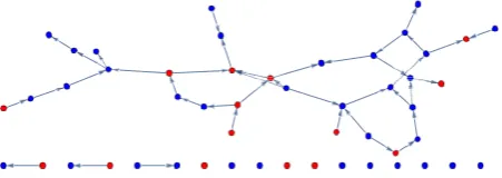
Figure 10 shows a typical directed random graph in the p(n) = λ_n, 0 < λ < 1, regime.

One can see one weakly connected component and some small trees and isolated points. The undirected graph in this regime consists exclusively of trees and a weakly connected component seems unlikely at rst. If one, however, considers the possible paths from any vertex in the graph, one comes to the conclusion that the graph still has a treelike structure. We will elaborate this thought further.

Figure 10: Coloured Binomial Directed Random Graph G(n, p) with n = 50,

p = 0.015and colour probability q = 0.3. The Graph is an example of a directed

random graph with edge probabilityp= λ_n withλ= 0.75.

Every vertexiin a directed graph has incoming and outgoing edges with degrees distributed

independently with

Incomming Degree: din(vi)∼Bin(n−1, p(n))

Outgoing Degree: dout(vi)∼Bin(n−1, p(n)) .

Forp(n) = λ_n, this can be approximated in the limit by a Poisson distribution with

din(vi)∼P oi(λ) ,

dout(vi)∼P oi(λ) .

Assume we want to explore the random graph, starting at vertexS. Starting atS, we only

consider outgoing edges of S to reach it's k neighbours. In each of it's k neighbours, we

again consider only outgoing edges to investigate new vertices. Continuing this step till no more new vertices can be found, equates to exploring all reachable vertices starting at vertexS. Observe that we only used outgoing edges to explore the graph. The distribution

of outgoing edges is equal to the distribution of edges in a undirected random graph in the same regime. The number of reachable vertices from a starting vertexS in a directed

random graph in thep= λ_n,0< λ <1, regime is equal to the number of reachable vertices

in a undirected random graph in the p = λ_n, 0 < λ < 1, regime. We assume the Always

Red statement to hold with the same probability. Using Theorem 5.5 we formulate the following conjecture:

Conjecture 6.5 (Always Red in coloured directed random graph withp(n) = λ_n,0< λ <1).

For a coloured directed random graph G(n, p) with edge probability p(n) = λ_n, 0< λ < 1,

and colour probabilityq∈(0,1),

1

eλ < P(S red)<

1

√

2π q

eλ−1_−λq whenn→ ∞ .

Moreover,0< P(S red)for all values ofq, and 0< P(S red)<1for e−

1

√

6.4 Always Red in coloured directed random graph G(n, p)

with p = λ_n, λ > 1

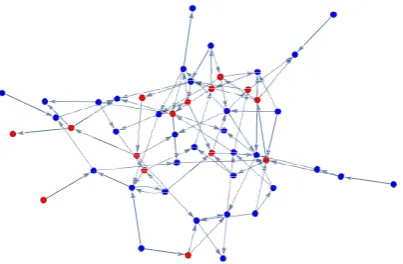
Figure 11 shows a typical random graph in the λ

n , λ > 1, regime. There is one weakly

connected giant component. At rst sight, the random graph looks nothing like the treelike structure present in the undirected graph in this regime. However, if we consider all possible path from a starting vertexS, we recognize the treelike structure.

Figure 11: Coloured Binomial Directed Random Graph G(n, p) with n = 50,

p = 0.03 and colour probability q = 0.3. The Graph is an example of a directed

random graph with edge probabilityp= λ_n withλ= 1.5.

If we start to explore the graph, starting at a starting vertexS, we assume to nd exactly

the graph structure present in the undirected graph in the same regime. Then, S lies

either in a tree or in a giant connected component. Using this reasoning we formulate the following conjecture.

Conjecture 6.6 (Always Red in coloured directed random graph withp(n) = _nλ,λ >1).

For a coloured directed random graph G(n, p) with edge probability p(n) = λ_n, λ >1, and

colour probability q∈(0,1), there exists values for λand q, such that

P(S red)6= 0 and

P(S red)6= 1 when n→ ∞ .

Proof. We will condition on whetherS lies in the giant component or not:

P(S red) =P(S red|S ∈ Cmax) P(S∈ Cmax)

+P(S red|S 6∈ C_max) P(S6∈ C_max) .

By Theorem 6.1, we know that the entire graph is not strongly connected and we conclude that with positive probability, S is outside of the giant component. When S is outside

of the giant component, the component of S can be described as a branching process

conditioned on extinction. The probability ofAlways Red conditioned on S being outside

of the the giant component is described in Conjecture 6.5. This probability is strict greater than zero. We conclude

P(S red)≥P(S red|S ∈ C_max) P(S∈ C_max)>0 .

replacing all the directed edges of a directed random graphGD(p, n) by undirected edges.

Parallel edges will be reduced to one edge. The degree of a vertexviof the graphG?U(p, n)

will hold

d_GD(p, n)(vi)≤d_G?U(p, n)(vi)≤2d_GD(p, n)(vi) .

The lower bound is obtained if every edge of vertex i in GD(p, n) has a reversed edge.

The upper bound is obtained if none of the edges has a reversed edge. We claim that the number of reachable states from a starting vertexSis higher in the graph ofG?_U(p, n)than

in the graph ofGD(p, n), due to the undirectedness of the edges. Subsequent more vertices

can be reached in the graph ofG?_U(p, n) than in the graph ofGD(p, n)and(S red)has

a lower probability in the graph ofG?_U(p, n)than in the graph of GD(p, n). That is

PG_D(S red)≤PG?_{_U}(S red) .

Due to its average degree given byλ≤d¯? ≤2λ, we claim that the graphG?_U(p, n)behaves

like a binomial undirected graphGU(p?, n) withp(n)< p?(n)<2p(n). The probability of

(S red)inGU(p?, n)is given in Section 5.4 and Theorem 5.8 states it is strictly smaller

than one for most of the values ofq and λ. Thus,

P(S red inGD(n, p))≤P(S redinG?U(p, n))<1 for some values ofλand q.

7 Conclusions

For a binomial undirected random graph, the Always Red statement occurs with probability tending to zero for as well thep(n) =cas thep(n) = clog(_nn) case, asntends to innity. In

these regimes it is possible that Linear Temporal Logic obeys a Zero-One law. However, in the p(n) = λ_n regime we found a counterexample for the Zero-One law for most of the

values of λ and q. Theorem 5.5 and Theorem 5.8 disprove a Zero-One law for Linear

Temporal Logic in undirected random graphs. For a binomial directed random graph the probability of Always Red will tend to zero for the p(n) = c and p(n) = clog(_nn) regimes,

as in the undirected case. A Zero-One law could exist in these regimes. For thep(n) = λ_n

regimes, we do not have any concrete probabilities yet, however, we have reasons to accept the probability of Always Red to be strictly bounded by zero and one for most values of

λandq, as stated in Conjecture 6.5 and Conjecture 6.6. We therefore assume the Always

Red statement to be a counterexample for a Zero-One Law for Linear Temporal Logic in directed random graphs. In conclusion, we disproved a Zero-One law for Linear Temporal Logic for graphs by counterexample.

References

[1] C Baier and Joost P. Katoen. Principles of Model Checking, pages 229233. MIT Press, 2008.

[2] M Aslam Chaudhry, Asghar Qadir, and Asifa Tassaddiq. Extended fermi-dirac and bose-einstein functions with applications to the family of zeta functions. arXiv:1004.0588, pages 14, 2010.

[4] Ronald Fagin. Probabilities on nite models. The Journal of Symbolic Logic, 41(1):50 58, 1976.

[5] Alan Frieze and Michaª Karo«ski. Introduction to Random Graphs. Cambridge Uni-versity Press, 2015.

[6] Alasdair J. Graham and David A. Pike. A note on thresholds and connectivity in random directed graphs. Atlantic Electronic Journal of Mathematics, 3(1), 2008. [7] Herbert Robbins. A remark on stirling's formula. The American Mathematical

Monthly, 62(1):26, 1955.

[8] Saharon Shelah and Joel Spencer. Zero-one laws for sparse random graphs. Journal of the American Mathematical Society, 1(1):97115, 1988.

[9] Joel Spencer. The Strange Logic of Random Graphs, pages 321. Springer-Verlag Berlin Heidelberg New York, 2001.