Heuristic solutions to the target identifiability problem in directional sensor networks

(1)

Original citation:

Tan, Wilson M. and Jarvis, Stephen A.. (2016) Heuristic solutions to the target

identifiability problem in directional sensor networks. Journal of Network and Computer Application, 65 . pp. 84-102.

Permanent WRAP url:

http://wrap.warwick.ac.uk/77939

Copyright and reuse:

The Warwick Research Archive Portal (WRAP) makes this work of researchers of the University of Warwick available open access under the following conditions. Copyright © and all moral rights to the version of the paper presented here belong to the individual author(s) and/or other copyright owners. To the extent reasonable and practicable the material made available in WRAP has been checked for eligibility before being made available.

Copies of full items can be used for personal research or study, educational, or not-for-profit purposes without prior permission or charge. Provided that the authors, title and full bibliographic details are credited, a hyperlink and/or URL is given for the original metadata page and the content is not changed in any way.

Publisher statement:

A note on versions:

The version presented here may differ from the published version or, version of record, if you wish to cite this item you are advised to consult the publisher’s version. Please see the ‘permanent WRAP url’ above for details on accessing the published version and note that access may require a subscription.

(2)

Heuristic Solutions to the Target Identifiability

Problem in Directional Sensor Networks

Wilson M. Tan and Stephen A. Jarvis

Performance Computing and Visualisation Group

Department of Computer Science

University of Warwick, UK

Abstract

Existing algorithms for orienting sensors in directional sensor

net-works have primarily concerned themselves with the problem of

max-imizing the number of covered targets, assuming that target

identi-fication is a non-issue. Such an assumption however, does not hold

true in all situations. In this paper, heuristic algorithms for choosing

active sensors and orienting them with the goal of balancing coverage

and identifiability are presented. The performance of the algorithms

are verified via extensive simulations, and shown to confer increased

target identifiability compared to algorithms originally designed to

(3)

1 Introduction and motivation

Directional sensors are sensors whose sensing capabilities are limited within

an angle range [7][8]. In comparison, an omnidirectional sensor’s sensing

range covers everything around it. In geometric terms, the covered area of

an omnidirectional sensor is a circle centered on the sensor, while that of a

directional sensor is a sector. In WSNs, nodes that are directionalcan imply

that the node has directional capability in sensing and/or communication

[7]. In this paper, we solely focus on the sensing capability, and thus will

interchangeably use the terms ‘nodes’ and ‘sensors’.

Examples of sensors that are inherently directional in nature include video

sensors [11], ultrasonic sensors [3], and infrared sensors [13]. Acoustic

sen-sors (or microphones) can also potentially be directional [9], although most

of the existing work in WSN literature so far have utilized omnidirectional

microphones [12][6].

Because the sensed region of a directional node is constrained within an

angle range, of primary concern is the total sensing coverage provided by

such a network of directional sensors. A problem that frequently needs to

be solved is ‘Given a number of directional sensors distributed in space, how

should each sensor’s sensing region be oriented such that the total sensing

coverage of the network is maximized?’.

Coverage-maximizing algorithms proposed in literature fall into two

cat-egories: those that are target-centric and those that are area-centric.

In target-centric algorithms, it is assumed that there are a finite number of

(4)

of such targets be covered. Sometimes, for issues of energy efficiency, it is

also desired that the covering be also done with the least number of sensors

possible - such a problem is formalized in [1] as the Maximum Coverage

Minimum Sensors (MCMS) Problem.

In area-centric algorithms, there are no specific objects or targets of

in-terest; the entire area is of sensing interest, and it is desired that as much

of it is covered. In such algorithms, the problem is equivalent to minimizing

the overlap between the sensed regions of sensors. An example of such an

algorithm was presented in [16].

In this work, we solely focus on target-centric algorithms.

Most coverage algorithms focus on maximizing the number of targets

cov-ered. This is reasonable when the targets are continually being monitored,

and easy target identification is built-in to the system. This is true to a

certain extent for visual sensor networks: for instance, a Closed Circuit

Tele-vision (CCTV) camera (being remotely watched by a person) monitoring a

street intersection. However, this assumption does not hold true for all

situ-ations. For instance, if we assume that a single acoustic sensor is monitoring

two possible sound sources, in general, the sensor will be able to detect that a

sound was generated, but not which source generated it - at least not unless

the sound generated by each source is distinct, and even then, not without

further digital signal processing.

As a slight deviation from all previous studies, we shall work with the

following assumptions

(5)

oc-cur only one at a time, and they are brief enough that they do not

overlap in time.

2. Events can be detected by the sensor if the source is within the

sen-sor’s sensed region, but the events themselves say nothing about which

source generated it.

s1 s2

1

2 3 4

1

a1

1

a2

1

a3

1

a4

1

a5

Figure 1: Diagram for the first example.

In this work, instead of just focusing on the number of targets covered,

we will also concern ourselves with the identifiability of the targets or event

sources.

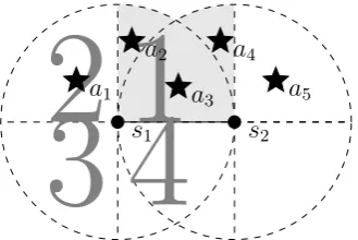
As a motivating example, we present Figure 1, where the dots s1 and

s2 are sensors while the stars a1 - a5 are the targets. The dotted regions

around each sensor represent the possible covered or sensed region of each

sensor. Each sensor can be oriented to be in 1 of 4 possible orientations.

Orientation 1 represents the region covered by the sector from 0° to 90°, 2

covers 90° to 180°, 3 covers 180° to 270°, and 4 covers 270° to 360°. In this

example, the boundaries of the sensed regions of each sensor are aligned with

the cardinal directions (and with each other). The 4 possible orientations for

[image:5.595.216.381.277.387.2]

(6)

is not required by the algorithms that will be discussed. In Figure 1 s1 is

in orientation 1, while s2 is in orientation 2. With these orientations, a2 is

covered by s1, a3 is covered bys1 and s2, and a4 is covered bya2. A total of

3 targets are covered. a1 and a5 are not covered.

It is easy to verify that 3 is the maximum number of targets that can be

covered by any network configuration. A network configuration is a set of

active sensors, each with its corresponding orientation.

However, the configurations1 - 1 (shorthand fors1 in orientation 1),s2

-2 is not the only configuration that yields 3 covered targets. s1 - 2,s2 - 2 also

yields 3 covered targets, as will s1 - 1, s2 - 1. There are differences however

in the identifiabilities conferred by these configurations to the targets that

they cover.

Let us begin with s1 - 2, s2 - 2. When a1 generates an event, s1 will be

able to detect it, and we know for certain that a1 generated the event since

it is the only target covered by s1. When a3 generates an event, s2 will be

able to detect it, but we are not sure whether it was a3 ora4 that generated

the event. The best that can be done is hazard a guess with 50% probability

of being correct. The same analysis holds for s1 - 1, s2 - 1.

Compare this with s1 - 1, s2 - 2. When a2 generates and event, s1 will

be able to detect it. At first glance, it seems like we might not be able to

distinguish whether it wasa2 ora3 which generated the event since both are

covered by s1. However, we can know that it isnota3, sinces2 did not detect

anything. Hence, it must be a2 which generated the event. In other words,

whether a target generated an event or not can be deduced not just from

(7)

anything.

We call the set of sensor states (where state indicates whether a sensor

detected something or not) which signifies a target generating an event as

the target’s syndrome. A syndrome is a tuple of values, one for each active

sensor in the system, each denoting whether a sensor will detect anything

upon the target generating an event. For a sensor x, let sx be the element

for the sensor in the tuple if the sensor will detect anything, and sx’ if it will

not. In our latest example, a2 has the syndrome s1s02. Table 1 enumerates

the syndrome for each covered target in each of the network configuration

that yields 3 covered targets.

s1 - 1, s2 - 2 s1 - 2, s2 - 2 s1 - 1, s2 - 1

a1 - s1s02

-a2 s1s02 - s1s02

a3 s1s2 s01s2 s1s02

a4 s01s2 s01s2

-a5 - - s01s2

Table 1: Configurations that yield 3 covered targets, and their resulting syndromes.

In Table 1, we can clearly see why the configuration s1-1, s2-2 affords

better target identifiability: in that configuration, each covered target has

its own syndrome. In comparison, in the other two configurations, two targets

have to share a single syndrome, resulting in ambiguity when identifying their

events.

It must be noted that some aspects of Figure 1 do not hold true in other

(8)

Firstly, sometimes, assigning a single syndrome for each target is simply

impossible. Nevertheless, it is conceivable that even in such situations, it is

desirable to minimize the ambiguity between events as much as possible.

Secondly, in other networks (especially those that are underprovisioned,

meaning there are few sensors relative to targets), it is possible that improved

target identifiability will come at the cost of less targets covered. The

accept-able trade-off between the number of targets covered and their identifiability

will vary from one application to the next.

Another use of the concept of identifiability is inoverprovisionednetworks

- that is, networks where there is a surplus in the number of sensors, and

even after the maximum possible number of targets has been covered, there

are still sensors that are not covering anything. In previous studies, the extra

sensors are used in extending the network lifetime: sensors form cover sets

that take turns covering the targets [2]. Clearly, another possible use for such

extra sensors is in increasing the identifiability of targets.

This paper makes three contributions: firstly, the introduction of the

con-cept ofsyndromes; secondly, the definition of the Maximum Target

Identifiability-Aware Utility with Minimum Sensors (MTIAUMS) problem; and finally, six

heuristic algorithms that determine network configurations that strike a

bal-ance between identifiability and the number of targets covered.

This paper is structured as follows. The notations utilized are discussed

in Section 2. The problem is formally defined, and its NP-hardness proven in

Section 3. Centralized heuristic algorithms are presented in Section 4, while

distributed heuristic algorithms are presented in Section 5. The methodology

(9)

in Section 6. A discussion of related work follows in Section 7, while Section 8

concludes the paper.

2 Notations

The following notations are used in this paper

• M: number of targets.

• ai: a specific target, 1≤ i ≤ M.

• A: the set of all targets A = {a1,a2, ... aM}.

• N: number of nodes.

• si: a specific node, 1 ≤ i ≤N.

• S: the set of all nodes S = {s1,s2, ... sN}.

• r: the sensing radius; a target is said to be covered by one of the node’s orientations if the distance between the target and the node is less than

or equal to the sensing radius.

• W: number of orientations with which each node can work with.

• φi,j: set of targets covered by nodeiwhen it is working with orientation

j, 1 ≤ i ≤ N, 0 ≤ j ≤ W. Note that we allow j to take on the value of 0: this indicates that the node’s sensing mechanism is inactive, thus

φi,0 = {}, ∀i.

• Φi: set of all targets within range of si, regardless of orientation; Φi =

(10)

• Qi: set of nodes comprised of one-hop neighbours of si.

• Φ0_i: set of all targets within range ofsi’s one-hop neighbours, sans those

also seen by si; Φ0i = {∪ Φj \ Φi | sj ∈ Qi}.

• α: user-defined parameter indicating the desired trade-off between the number of targets covered and their identifiability; higher value

indi-cates more preference for number of targets covered; 0 ≤ α ≤ 1.

• Z: network configuration, set of active sensors and corresponding ori-entations; set of (i, j) pairs, where i ∈ S, 1≤ j ≤ W.

• ui: target utility for a given Z, 1≤ i ≤ M.

• U: sum of all target utilities for a given Z.

2.1 Coverage by a specific orientation

Once a target is ascertained to be within a node’s sensing radius, the specific

orientation of the node covering the target can be determined by

1. Let D be the node, E the target, and F a point immediately to the right of the node. From these points, define the vectors DE and DF

(which should be parallel to the x-axis).

2. Compute the angleθ using

θ= DE·DF

(11)

3. In this study, we assume that the orientation numbers are assigned

in a counter-clockwise fashion. The orientation numbers are assigned

starting from a reference axis, which in this study is coincidental with

the x-axis. Let the offset (in degrees) of the reference axis be referred

to asrefof f set. The specific orientationn which covers a certain target

can then be determined using

(360°

W +refof f set)×(n−1)≤θ <(

360°

W +refof f set)×n (2)

3 Problem definition

To give consideration to the fact that not all setups will be like that in

Figure 1 (where the network configuration which maximizes the number of

targets covered also maximizes the number of syndromes), we first introduce

the concept of target utility, ui

ui =α+ (1−α)(certaintyi) (3)

ui will depend on the network configuration Z. α is a parameter (with

value between 0 and 1, inclusive) defined by the user, which indicates the

desired trade-off between the number of targets covered and identifiability: a

higherαindicates that the number of covered targets is more important than the number of syndromes in the system, a lowerαvalue indicates the reverse.

certaintyi is the level of certainty with which a target can be identified when

(12)

is dependent on Z). It can be defined as

certaintyi =

1

# of targets sharing the same syndrome as ai

(4)

Building on the concept of target utility, we define system utility,U:

U =

M

X

i=1

ui (5)

Another definition forU will be

U =α(number of targets covered) +

(1−α)(number of syndromes in the system) (6)

The second term holds because if all the certainties of all covered targets

are summed, one will end up with the number of syndromes in the system.

Unless explicitly stated, references to ‘utility’ in this paper must be taken to

mean ‘system utility’.

Our goal is to provide coverage to targets, maximizing the system

util-ity as defined by Equation 6, while activating as few sensors as possible.

We call this problem the Maximum Target Identifiability-Aware Utility with

Minimum Sensors (MTIAUMS) problem. A more formal statement of the

problem will be: Given a set of targets A and a set of sensors S (each with

W possible sensing orientations), find a network configuration Z (consisting

of a set of active sensors, along with their corresponding orientations), such

(13)

minimized.

It must be noted that the computed system utility is affected by the

ratio of targets to sensors, and their densities (targets per unit area, sensors

per unit area). If there are significantly more targets than sensors (several

orders of magnitude higher, for instance), it is actually possible for heuristic

algorithms that only aim to maximize the number of covered targets to attain

a higher system utility than our algorithms. While the algorithms will still

confer better identifiability to covered targets in such a situation, that can

possibly be hidden by the fact that there are significantly more possible

targets that can be covered (first term, Equation 6) than there are possible

syndromes that can be generated (second term, Equation 6). In such cases,

it might be helpful to take the metric _syndrometargets into account when evaluating

solutions. In this work, we will deal with cases wherein the number of targets

is comparable to the number of sensors.

In this study, we propose heuristic solutions to the MTIAUMS problem.

A Heuristic solution is useful since the problem is NP-hard (this will be

proven in the next subsection).

3.1 NP-hardness of the problem

We prove the NP-hardness of the problem through the ‘Proof by

Restric-tion’ method [5]. When α = 1, the MTIAUMS problem becomes the Maxi-mum Coverage with MiniMaxi-mum Sensors (MCMS) problem defined in [1]. The

MCMS problem therefore is a special case of the MTIAUMS problem. It is

(14)

problem is also NP-hard.

4 Centralized algorithms

Centralized algorithms are presented first. Syndrome counting is discussed

in Section 4.1. Our first heuristic algorithm, TIA-CGA, is presented in

Sec-tion 4.2. Two other centralized algorithms are discussed in SecSec-tion 4.3.

4.1 Counting syndromes

The capability to count the number of syndromes associated with a specific

network configuration is of primary importance to algorithms that will be

presented later. To count the covered targets and to evaluate the level of

identifiability afforded by a given network configuration (or set of sensor

orientations), we introduce the concept ofcoverage matrix. A coverage matrix

is formed from a given Z. A coverage matrix has its rows indexed by the members of A and its columns indexed by the members of S. Let zi,j be a

member of a coverage matrix

zi,j =

 



1 ifi ∈ φj,k s.t. (j, k) ∈ Z;

0 otherwise, inc. (j, k)∈/ Z ∀ k, 1 ≤ k ≤ W.

(7)

To count the number of syndromes in a given configuration, we use

Algo-rithm 1. One of the inputs to AlgoAlgo-rithm 1 is an array called covered whose

element is 1 if the index corresponding to the target is covered in the

cov-erage matrix (at least one non-zero value in the corresponding row). The

(15)

Equation 7.

Algorithm 1 Syndrome counting algorithm

1: Inputs: coverage matrix with elementszi,j (generated using Equation 7);

an array called covered whose element is 1 if the index corresponding to the target is covered in the coverage matrix (at least one non-zero value in the corresponding row)

2: Output: syndromes - the number of syndromes in the system when

solution embodied by the coverage matrix is applied

3: syndromes ← 0

4: processed(i) ←0 ∀i∈A 5: for 1≤i≤M do

6: if (processed(i) == 0) && (covered(i) == 1) then

7: syndromes← syndromes + 1 8: for i+ 1 ≤j ≤M do

9: if (processed(j) == 0) && (covered(j) == 1) then

10: same ←1

11: for 1≤k≤N do

12: if zi,k !=zj,k then

13: same ← 0

14: end if

15: end for

16: if same == 1 then

17: processed(j) ←1

18: end if

19: end if

20: end for

21: processed(i)← 1

22: end if

23: end for

Algorithm 1 works by comparing the syndromes of each target in a

pair-wise fashion. In the coverage matrix, the syndrome of a target is represented

by the values in the row corresponding to the target number. For

exam-ple, target a1’s syndrome will be the concatenation of the values in row 1:

z1,j,0≤j ≤N. Each target, unless already ‘processed’, becomes a reference

(16)

sequentially (Algorithm 1, Line 5). The reference row is then compared with

rows with higher numbers (Algorithm 1, Line 8). The actual

element-by-element comparison of the syndromes happens in Algorithm 1 Lines 11-15.

If a row has exactly the same values as the reference row, it is marked as

already processed (Algorithm 1, Line 21) and loses the chance to become

a reference row itself. It will also not be eligible for comparison with any

other future reference rows. The successful selection of a new reference row

effectively represents the ‘discovery’ of a new syndrome and the syndromes

variable is incremented by 1 (Algorithm 1, Line 7).

The maximum number of target-target comparisons that can possibly be

performed in the process of counting syndromes is equivalent to the number

of pairwise combination of targets (Algorithm 1, Lines 6 and 9), or _2!(_MM₋!_2)!.

Within a target-target comparison, it is checked whether or not both

tar-gets are covered by each sensor (N, Algorithm 1, Line 11). Therefore, the

computational complexity of Algorithm 1 is _2!(N M_M₋!_2)!.

4.2 Target Identifiability-Aware Centralized Greedy

Al-gorithm

The Target Identifiability-Aware Centralized Greedy Algorithm (TIA-CGA)

is a heuristic algorithm that produces network configurations that take into

account both the number of targets covered and the identifiability of those

targets. The TIA-CGA is primarily derived from the Centralized Greedy

Algorithm (CGA) presented in [1]. The CGA is a greedy algorithm which

(17)

Algorithm 2 Target Identifiability-Aware Centralized Greedy Algorithm

1: Inputs: A;S; α; φi,js

2: Output: Z - network configuration, a set of (ID of active node,

config-uration of active node) pairs

3: Z ← ∅

4: V ← A . at the end, will contain all uncovered targets 5: Y ← S . at the end, will contain all inactive nodes

6: new_utility ← 0

7: while 1 do

8: old_utility ← new_utility

9: for (i, j) s.t. si ∈ Y, 0≤j ≤W do

10: T empN odeSet ← ∅

11: T empN odeSet ←Z ∪{(i, j)}

12: T empCovM atrix ← coverage matrix generated from

T empN odeSet .generate using Equation 7

13: Qi,j ←SyndromeCount(T empCovM atrix, associatedcovered

ar-ray) .compute number of syndromes using Algorithm 1

14: Ui,j ← (α) ×(|φi,j∩V|) + (1 -α)× (Qi,j)

15: end for

16: (i, j)← arg maxsi∈Y,0≤j≤W Ui,j

17: new_utility ←maximum U i, j determined in previous step

18: if new_utility - old_utility ≤ 0 then

19: break . utility does not increase anymore, algorithm ends

20: else

21: Z ← Z ∪ {(i, j)}

22: V ← V \φi,j

23: Y ← Y \{(si)}

24: end if

25: end while

which adds the highest number of targets to those already covered. The

CGA main loop can be seen in Algorithm 3, Lines 7-22 sans Lines 8-11

and 14. The main difference between the TIA-CGA and the CGA is that

in an iteration, instead of choosing the sensor-orientation pair which adds

the most number of newly covered targets, the TIA-CGA chooses the pair

(18)

this, for each remaining unchosen sensor-orientation pair, it computes the

number of additional targets that will be covered if the pair was chosen next,

and the number of syndromes that the system will have (Algorithm 2, Lines

10-13). These two values are weighted by the priority factors α and 1 - α, respectively, and then added together (Algorithm 2, Line 14). Algorithm 2

Line 16 chooses the pair which adds the greatest system utility to the system.

The algorithm will stop when the best pair found no longer improves the

system utility (Algorithm 2, Lines 18-19); otherwise, the pair is added to the

solution (Algorithm 2, Line 21), the sensor is removed from the set of sensors

viable for selection in the next iteration (Algorithm 2, Line 23), and the loop

begins anew.

To derive the computational complexity of Algorithm 2, it must be noted

that in each of its iteration, it needs two pieces of information to choose

the orientation pair: the number of additional targets each

sensor-orientation pair will cover (if chosen), and the number of syndromes each

sensor-orientation pair will add to the system (if chosen).

The number of targets covered can be determined in MNW steps, in

keeping with the value derived in [1].

For the number of syndromes, there are NW sensor-orientation pairs to

evaluate. In each evaluation, a coverage matrix is generated (Algorithm 2,

Line 13, Equation 7). The coverage matrix has MN elements, so it can

be assumed that it will take MN steps to evaluate. The coverage matrix

is processed by Algorithm 1, with complexity ₂₍N M_M₋_2)!! . Therefore, in each

iteration of the main loop of Algorithm 2, the complexity due to syndrome

(19)

The evaluation of the system utility and the choosing of the sensor-sensor

configuration pair can be done in NW steps. There are a maximum N

iter-ations of the main loop of Algorithm 2. Therefore, the overall complexity of

Algorithm 2 is N(M N W +N W(M N +₂₍_MN M₋_2)!! ) +N W).

4.3 2-stage algorithms

The next algorithms that will be introduced are the 2-stage algorithms. One

of these algorithms is based on the Centralized Force-based Algorithm (CFA),

so a short introduction on CFA is in order.

The CFA is an alternative to CGA, proposed in [10]. Like CGA, CFA

aims to produce network configurations that maximize the number of

tar-gets covered, and does so greedily. Unlike CGA however, when building the

solution, it does not solely rely on the number of targets that will be

cov-ered by each sensor-sensor configuration pair. Instead, at each step of the

computation, it chooses on the basis of the ‘force’ exerted by a sensor

con-figuration (or direction) on the sensor. This force is defined as the ratio of

the targets covered by a specific sensor configuration to the total number of

targets covered by the sensor (Equation 8).

Fi,j =

|φi,j|

|Φi|

(8)

The 2-stage algorithms basically apply CGA or CFA first to the problem

and then attempt to increase the number of syndromes in the system by

greedily using the sensors left unselected. When the first stage is CGA, the

(20)

Algorithm 3 2-stage Target Identifiability-Aware Greedy Algorithm

1: Inputs: A;S; φi,js; CFAStage1 - binary variable, 1 if desired first stage

is CFA, 0 if CGA

2: Output: Z - network configuration, a set of (ID of active node,

config-uration of active node) pairs

3: Z ← ∅

4: V ← A . at the end, will contain all uncovered targets

5: Y ← S . at the end, will contain all inactive nodes

6: new_syndrome_count ← 0

7: while 1 do

8: if CFAStage1 == 1 then .First stage is CFA

9: Compute Fi,j =

|φi,j∩V|

|Φi∩V| ∀ si ∈ Y, 0≤j ≤W

10: (i, j)← arg maxsi∈Y,0≤j≤W Fi,j

11: else . First stage is CGA

12: Compute |φi,j ∩V| ∀si ∈Y, 0≤j ≤W

13: (i, j)← arg maxsi∈Y,0≤j≤W |φi,j∩V|

14: end if

15: if |φi,j ∩V| == 0 then

16: break . nothing new can be covered anymore, stage 1 ends

17: else

18: Z ← Z ∪ {(i, j)}

19: V ← V \φi,j

20: Y ← Y \{(si)}

21: end if

22: end while

Algorithm (2S-CGA), and when the first stage is CFA, the algorithm is called

2-stage Target Identifiability-Aware Centralized Force-based Algorithm

(2S-CFA).

In Algorithm 3, the first stage can be found in Lines 7-22. As previously

mentioned, the first stage can either be CGA or CFA. In the interest of saving

space, Algorithm 3 is made to be capable of using both CGA and CFA, with

the choice of which algorithm to use now dependent on the binary variable

CFAStage1, which is assumed to be an algorithm input. CFAStage1 having

(21)

23: while 1 do

24: old_syndrome_count← new_syndrome_count

25: for (i, j) s.t. si ∈ Y, 0≤j ≤W do

26: T empN odeSet ← ∅

27: T empN odeSet ←Z ∪{(i, j)}

28: T empCovM atrix ← coverage matrix generated from

T empN odeSet .generate using Equation 7

29: Qi,j ←SyndromeCount(T empCovM atrix, associatedcovered

ar-ray) .compute number of syndromes using Algorithm 1

30: end for

31: (i, j)← arg maxsi∈Y,0≤j≤W Qi, j

32: new_syndrome_count←maximumQi, jdetermined in previous step

33: if new_syndrome_count - old_syndrome_count ≤ 0 then

34: break . nothing can be covered that will increase the number of syndromes anymore, stage 2 and algorithm ends

35: else

36: Z ← Z ∪ {(i, j)}

37: Y ← Y \{(si)}

38: end if

39: end while

while CFAStage1 having the value of 0 denotes that CGA should be used

(Algorithm 3, Lines 113). We call this algorithm, which represents both

2-stage algorithms, the 2-stage Target Identifiability-Aware Greedy Algorithm.

The second stage can be found in Algorithm 3 Lines 23-39. In each

iteration of the loop, the number of additional syndromes that can possibly be

added by each remaining sensor-orientation pair is computed (Algorithm 3,

Lines 25-30). If the most that can be added by any sensor-orientation pair is 0

(or negative), the stage and the algorithm will end (Algorithm 3, Lines 33-34);

otherwise, the sensor-orientation pair is added to the solution (Algorithm 3,

Line 36), the sensor is removed from the set of viable or inactive sensors

(22)

It must be noted that strictly speaking, the two 2-stage algorithms are not

exact alternatives to the TIA-CGA. TIA-CGA always aims to maximize the

system utility, thus taking into account both targets covered and syndromes

generated at each step. The 2-stage algorithms only take the syndromes

into account after all targets that can possibly be covered are covered. In

situations where all sensors are utilized for covering targets (no leftovers)

-the 2-stage algorithms degenerate into CGA or CFA (depending on which

version is being used).

The complexity of the first stage of Algorithm 3 follows that of CGA or

CFA: N1(M N1W +N1W). N1 is the number of sensors that will be chosen

by the first step. If all sensors are utilized in covering targets (no leftovers),

N1 = N, and the complexity of Algorithm 3 becomes the same as that of

CGA or CFA.

The complexity of the second stage isN2(N2W(M N2+₂₍N_M2M₋_2)!! ) +N2W).

This is the same as that of Algorithm 2, but without the component for

count-ing covered targets. N2 is the number of unselected sensors left after the first

stage. The sum of N1 and N2 cannot exceed N (i.e., N1 + N2 ≤ N). The

complexity of Algorithm 3 is then N1(M N1W +N1W) +N2(N2W(M N2+

N2M!

2(M−2)!) + N2W), N1 + N2 ≤ N. The majority of the complexity of

Al-gorithm 2 stems from the computation necessary to count syndromes - by

sparing some (if not most) sensors from such a step (by splitting N into N1

and N2), the two 2-stage algorithms usually end up with shorter runtimes

(23)

5 Distributed algorithms

Communication costs (in terms of energy and time) will make the

trans-mission of data between the nodes and the base station (which will run the

algorithm in a centralized solution) prohibitive as the network grows in size

-hence, a distributed solution is at times more practical than a centralized one.

Relevant data structures to the distributed algorithms will first be discussed

in Section 5.1. Our first distributed algorithm, 2S-TIA-DGA, is introduced

in Section 5.2 and its operation discussed in Section 5.3. A comparison with

two algorithms for solving MCMS will be given in Section 5.4, and its time

complexity is discussed in Section 5.5. 2-stage heuristic algorithms are

intro-duced and discussed in Section 5.6.

5.1 Data structures

s1 s3

s2

1

a1

1

a2 1

a3

1

a4

1

a5

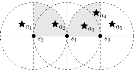
Figure 2: Diagram for the fourth example.

We first introduce two data structures on which the algorithm will rely

on. The data structures can be found in each node (as each node will run

the algorithm).

The first data structure is the seen_targets matrix. The seen_targets

[image:23.595.189.407.452.566.2]

(24)

by the members of Qi. A member of the seen_targets matrix (let us call it

zj,k) is defined by

zj,k =

(_{1 if}_s

k’s current orientation covers aj;

0 otherwise.

(9)

Assume that we have the setup in Figure 2, and that we are taking the

point of view of s1 (which has not yet decided on its orientation). Also

assume that s1 has a lower priority than either s2 or s3 (priorities will be

discussed later) and that it has just received a protocol message from each

of the nodes, informing it of their chosen orientations. The seen_targets

matrix of s1 will then be:

Q1

s2 s3

Φ1

a2 1 0

a3 0 1

The second data structure is theunseen_targetsmatrix. Like theseen_targets

matrix, it has its columns indexed byQi. The rows on the other hand, are

in-dexed by Φ0

i. The rows can be built dynamically (added as the node receives

messages from its neighbors), or be built at an initial information exchange

stage. The members of the unseen_targets matrix are defined in the same

way as the members of the seen_targets matrix (Equation 9). Continuing

with our example, if we take the point of view of s1, the unseen_targets

(25)

Q1

s2 s3

Φ0₁

a1 0 0

a4 0 1

a5 0 0

5.2 Algorithm overview

The algorithm Target Identifiability-Aware Distributed Greedy Algorithm

(TIA-DGA) is shown in Algorithm 4. In TIA-DGA, each node chooses the

orientation that has the highest total system utility and then announces its

choice to its neighbouring nodes. To avoid double counting, a node will

only count a certain target if it has not been covered yet by a node with

higher priority. An order of priority between the nodes (or at least within

neighbouring nodes) is necessary to ensure that the distributed algorithm will

eventually terminate [1]. Priorities in TIA-DGA are assigned by the number

of targets that a node can see, or |Φi|. The idea behind this is that nodes

that can cover a large number of targets (and thus, have higher priorities)

will take care of covering targets while nodes that do not have as many will

then increase the number of syndromes. Ties are broken using the node ID

numbers (which are assumed to be unique throughout the network).

5.3 Algorithm operation

Upon being initialized, a node will set its priority to the number of targets

that it covers in all orientations (Algorithm 4, Line 3). It will then proceed

(26)

Algorithm 4 Target Identifiability-Aware Distributed Greedy Algorithm

1: Inputs: α; φi,js; W; Qi; Φi; Φ0i;

2: Output: j_chosen - chosen orientation for the sensor node

3: Set priority P Ri =|Φi|

4: SetAndAnnounceBestOrientation();

5: whilea protocol message is received from sensor n∈Qi s.t. P Rn≥P Ri

do

6: if P Rn == P Ri then

7: if n >i then

8: continue;

9: else

10: stop processing message, throw it away

11: end if

12: end if

13: Based on the content of the message and Equation 9, update

seen_targets matrix and unseen_targets matrix

14: SetAndAnnounceBestOrientation();

15: end while

For each of the possible orientations, the number of targets that can

possibly be acquired can be determined by counting the number of relevant

rows in the seen_targets matrix with all-zero entries (Algorithm 5, Line 3):

because the relevant rows are those whose index belong to φi,j, each row is

representative of a target that can be seen by the sensor; the row having

all-zero entries signifies that it has not been covered yet by any other sensor.

The algorithm will then determine how many additional syndromes it can

create by choosing the orientation under consideration. This can be done by

counting the unique row patterns (we definepatternhere as the concatenation

of the column-by-column values) in theseen_targetsmatrix that have at least

one equivalent row pattern in the unseen_targetsmatrix (Algorithm 5, Line

4). The idea behind this is that a new syndrome is actually assigned to a

(27)

Algorithm 5 Algorithm for setting and announcing best orientation (Se-tAndAnnounceBestOrientation)

1: j_old ← j_chosen 2: for j s.t. 1≤j ≤W do

3: Pj ← number of rows in seen_targets matrix with all 0s, s.t. target

corresponding to the row ∈ φi,j

4: Rj ← number of unique rows in seen_targets matrix that can also

be found in unseen_targets matrix, s.t. target corresponding to the

seen_targets matrix row∈ φi,j

5: if Pj != 0 then

6: Rj ←Rj + 1

7: end if

8: Uj ← (α)× (Pj) + (1 -α)× (Rj)

9: end for

10: if arg max1≤j≤W Uj == 0 then

11: j_chosen← 0

12: else

13: j_chosen← arg max1≤j≤W Uj

14: end if

15: if j_chosen != j_old then

16: Set orientation to j_chosen

17: Send a protocol message including priority andφi,j_chosen

18: end if

new syndrome is added to the system as the assigned syndrome can simply

be a redefinition of the previous syndrome. Theaddition of a new syndrome

to the system will only happen if and only if

1. There are other targets that share the target’s current syndrome, and

2. Those targets will notshare the new syndrome that will be assigned.

Going back to the previous example, shoulds1 choose orientation 1, it will

add a new syndrome to the system: a3 will be given a syndrome different

(28)

s1 choose orientation 2, the syndrome of a2 will be redefined, but no new

syndrome will be added to the system, since only a2 uses the old syndrome.

After the number of possibly newly covered targets and possibly newly

added syndromes are counted, they are then weighted and added, resulting

in the utility (Algorithm 5, Line 8) for the orientation. This is done for each

possible orientation.

If there is no utility that can be had from choosing any orientation, the

node will turn the sensing mechanism off (Algorithm 5, Line 11). It is

as-sumed however, that even with the sensing mechanism turned off, the node

can still send and receive protocol messages. If there is at least one

orien-tation with a non-zero additional utility, the orienorien-tation with the highest

additional utility is chosen (Algorithm 5, Line 13), and the orientation set to

it (Algorithm 5, Line 16). The node will then broadcast a protocol message

containing its priority, and the targets that it has chosen to cover with its

orientation (Algorithm 5, Line 17). To minimize congestion and save energy,

a protocol message is only sent if the node changed its chosen orientation

(Algorithm 5, Line 15). Take note that the protocol message will contain

φi,j, meaning, it contains all targets covered by the chosen orientation, even

those already covered by another node.

Assuming that the node is still in its initialization stage, the matrices

seen_targets and unseen_targetswill not contain anything (basically, this is

the same as the node assuming that all of its neighbours are turned off).

After the initialization stage, the node will begin receiving messages from

its neighbours. After determining that a message should be processed (i.e.,

(29)

matri-ces seen_targets and unseen_targets with the contents of the message

(Al-gorithm 4, Line 13), and the function SetAndAnnounceBestOrientation is

executed.

5.4 Comparison with DGA and DFA

We compare our algorithm with the Distributed Greedy Algorithm (DGA)

[1] and the Distributed Force-based Algorithm (DFA) [10], two distributed

heuristic algorithms designed to maximize the number of targets covered by

a network of directional sensors.

In DGA, the priorities are randomly assigned, and the nodes choose the

orientation with the highest number of targets not covered by neighbouring

nodes with higher priorities.

In DFA, the priorities are determined by the highest ‘force’ the node

experiences in any orientation, with the force in a given orientation defined

by Equation 8. If the force values of two neighbouring nodes are similar,

the number of targets covered are then compared; if those are also equal,

node ID values are used to ultimately break the tie. Like in DGA, the nodes

choose the orientation with the highest number of targets not covered by

neighbouring nodes with higher priorities.

5.5 Time complexity

Similar to DGA (and DFA), nodes in TIA-DGA have definite priorities,

en-suring termination in finite time. Another implication of this is that it also

(30)

hap-pens when sensors reach their final states one-by-one in the order of their

priorities), which is O(n2) [1].

5.6 2-stage distributed algorithms

We also introduce 2-stage algorithms for solving the MTIAUMS problem in a

distributed way. Similar to their centralized counterparts, the idea behind the

distributed 2-stage algorithms is to cover the targets first using distributed

heuristic algorithms designed for solving the MCMS problem (first stage).

The number of syndromes is then increased using the remaining sensors

(sec-ond stage). We introduce two 2-stage algorithms: 2-stage Distributed Greedy

Algorithm DGA) and 2-stage Distributed Force-based Algorithm

(2S-DFA). The difference between the two lies in the MCMS-solving algorithm

used in the first stage: 2S-DGA uses DGA for its first stage, while 2S-DFA

uses DFA for its first stage. An algorithm both representing 2S-DGA and

2S-DFA is presented in Algorithm 6.

The primary difference between DGA and DFA lies with how the priorities

of the nodes are determined. DGA randomly assigns priorities, assuming that

the random numbers assigned are unique among the nodes (Algorithm 6, Line

5). DFA assigns priorities based on the orientation with the most number of

targets covered (Algorithm 6, Lines 7-8). Since the priority values assigned

by DFA are not necessarily unique, a mechanism for tie-breaking is needed

(Algorithm 6, Lines 13-23). Algorithm 6 decides on the priority to assign

using the binary variableDFAStage1(Algorithm 6, Line 4), which is assumed

(31)

being represented is 2S-DGA, while a value of 1 denotes that the algorithm

being represented is 2S-DFA. The stage the algorithm is in is denoted by

the variableCurrentStatei. The first stage of the algorithm can be found in

Algorithm 6 Lines 11-26 while the second stage can be found in Algorithm 6

Lines 29-43.

In the first stage, a message received by the node is processed as long as

the message is from a node with a higher priority or while the supporting

function TimerFired returns F alse (Algorithm 6, Line 11). TimerFired is a function which returns F alse when the timer has not fired yet, and T rue

after the timer has fired. We assume that the timer is a countdown timer

which fires after a certain amount of time has elapsed after the timer is

started. The timer is started (and the amount of time the timer will wait

for specified) using the supporting function StartTimer. The timer is

simul-taneously stopped and reset using the supporting function StopTimer. The

three supporting functions are tabulated and described in Table 2.

The messages processed in the first stage cause the data structuresseen_targets

and unseen_targets to be updated (Algorithm 6, Line 24), and the

func-tion TwoStageSetAndAnnounceBestOrientation (Algorithm 7) to be called.

Similar to its counterpart for TIA-DGA,

TwoStageSetAndAnnounceBestOri-entation chooses the orientation with the highest additional utility. Unlike

Algorithm 5 however, Algorithm 7 defines utility differently. While

Algo-rithm 5 defines utility as a weighted sum of the number of covered targets

and the number of syndromes (Algorithm 5, Line 8) utility for Algorithm 7

in the first stage is solely determined by the number of covered targets

(32)

Function Input Return value Description parameters

StartTimer time before none starts the timer timer fires

StopTimer none none stops and resets the

timer TimerFired none binary returns T rue if

timer has fired; returnsF alse

if otherwise

Table 2: Supporting functions for Algorithm 6 and Algorithm 7

is broadcast (Algorithm 7, Line 21). At the end of Algorithm 7, the timer is

started with the supporting function StartTimer, and the timer duration is

specified to be equivalent to the value TIMEOUT. TIMEOUTis an amount

of time sufficient for the entire network to be covered by DGA or DFA. The

timer is stopped or reset every time a message is received (Algorithm 6, Line

12), assuming of course that the timer has not fired first. The situation of

a message from a neighbouring node in Stage 1 arriving after the node’s

timer has fired or elapsed should never happen if the variable TIMEOUT

was properly set.

The firing of the timer indicates that that the first stage is over and the

algorithm now moves to the second stage (Algorithm 6, Line 27). It must be

noted that nodes that got an orientation assignment from the first stage will

no longer participate in the second stage (Algorithm 6, Line 28).

(33)

primarily in that the timer no longer plays a role in the admission of packets

or messages (Algorithm 6, Line 29) and Algorithm 7 now defines utility based

on the number of syndromes generated (Algorithm 7, Line 11).

Algorithm 6 2-stage Target Identifiability-Aware Distributed Generic

Al-gorithm

1: Inputs: α;φi,js; W;Qi; Φi; Φ0i; DFAStage1 - binary variable, 1 if desired

first stage is is DFA, 0 if DGA

2: Output: j_chosen - chosen orientation for the sensor node

3: Set CurrentStatei = 1

4: if DF AStage1 == 0 then

5: Set priorityP Ri = unique random number

6: else

7: j_highest ←arg max1≤j≤W |φi,j|

8: Set priorityP Ri =|φi,j_highest|

9: end if

10: TwoStageSetAndAnnounceBestOrientation();

11: while(TimerFired() ==F ALSE)AN D(a protocol message is received

from sensor n ∈ Qi s.t. P Rn ≥ P Ri) do

12: TimerStop();

13: if P Rn == P Ri then

14: if Φi > Φn then

15: continue;

16: else

17: if n > ithen

18: continue;

19: else

21: end if

22: end if

23: end if

26: end while

(34)

28: if j_chosen == 0then

29: while a protocol message is received from sensor n∈ Qi s.t. P Rn ≥

P Ri do

30: if P Rn == P Ri then

31: if Φi > Φn then

32: continue;

33: else

34: if n > i then

35: continue;

36: else

38: end if

39: end if

40: end if

43: end while

44: end if

6 Methodology and simulation results

6.1 Methodology

We implement the algorithms and run the experiments in Matlab.

Differ-ent parameters are varied in differDiffer-ent simulations; however, unless otherwise

stated, default parameters for a setup are: 50 targets and 50 sensors

ran-domly distributed over a 50 x 50 space, with each sensor having a sensing

radius of 10, and 4 possible sensing orientations. Similar to Figure 1, the

axes dividing the sensing regions are aligned to a North-East-West-South

orientation; however, it should be noted that the results should not be any

different if it is otherwise. Also, unless otherwise stated, results presented

[image:34.595.106.490.126.459.2]

(35)

Algorithm 7Algorithm for setting and announcing best orientation, 2-stage version (TwoStageSetAndAnnounceBestOrientation)

1: j_old ← j_chosen 2: for j s.t. 1≤j ≤W do

3: Pj ← number of rows in seen_targets matrix with all 0s, s.t. target

corresponding to the row ∈ φi,j

4: Rj ← number of unique rows in seen_targets matrix that can also

be found in unseen_targets matrix, s.t. target corresponding to the

seen_targets matrix row∈ φi,j

5: if Pj != 0 then

6: Rj ←Rj + 1

7: end if

8: if CurrentStatei = 1 then

9: Uj ← Pj

10: else

11: Uj ← Rj

12: end if

13: end for

14: if arg max1≤j≤W Uj == 0 then

15: j_chosen← 0

16: else

17: j_chosen← arg max1≤j≤W Uj

18: end if

19: if j_chosen != j_old then

20: Set orientation to j_chosen

21: Send a protocol message including priority andφi,j_chosen

22: end if

23: if CurrentStatei = 1 then

24: StartTimer(TIMEOUT);

25: end if

The effect of α on the heuristic algorithms’ performance is evaluated in Section 6.2. The effect of the number of sensors, number of targets, etc.,

is evaluated in Section 6.3. Section 6.4 will compare the execution times of

TIA-CGA and the two centralized 2-stage algorithms. A limited validation

of the heuristic algorithms’ performance against that optimal solutions is

(36)

6.2 Effect of

α

on heuristic algorithms

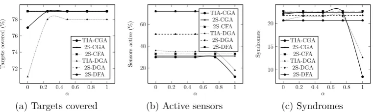
We test the effect of the parameter α on the performance of TIA-CGA and TIA-DGA using a setup with 50 targets and 50 sensors. Figure 3 plots the %

of targets covered, % of sensors that are active, and the number of syndromes.

Five values for α are tested: 0, 0.25, 0.5, 0.75, and 1.0. To provide a point of comparison, we also plot the metrics for 2S-CGA, 2S-CFA, 2S-DGA, and

2S-DFA. As expected, the plots for the four are horizontal lines, since they

are not parameterizable by α.

The first thing that must be noted from Figure 3 is how similar the

results are for α = 0.25, α = 0.5, and α = 0.75. This signifies that while the algorithms allow users to specify the acceptable level of trade-off between

coverage and identifiability, in reality and practice, sensor-target setups offer

a limited number of possible configurations and solutions. Therefore different

values of α(except 0 and 1.0) can result in the same solution. This does not mean however that α does not matter, as the results for α = 0 and α = 1.0 will show.

When α = 0, the algorithm degenerates into a syndrome-maximizing algorithm.

For TIA-CGA, α = 0 utilizes the same number of sensors as the three middle α values: 30% of the total (Figure 3b). With α = 0, the TIA-CGA covers slightly fewer targets than the solution for all other α values (Figure 3a) - 77% compared to α = 0.25’s 79%, for instance. Surprisingly,α

= 0 actually has a slightly lower average number of syndromes compared to

(37)

For TIA-DGA, α = 0 utilizes a slightly higher number of sensors than the three middle α values: 36% compared to 35% for α = 0.25 (Figure 3b). With α = 0, TIA-DGA covers less targets than the solution for all other α

values (Figure 3a) - 71% compared toα= 0.25’s 78%, for instance. Like TIA-CGA, atα= 0, TIA-DGA actually has a lower average number of syndromes compared to the three middle α values (Figure 3c).

α= 1.0 signifies that only the number of covered target matters, and the algorithm degenerates into a coverage-maximizing algorithm.

TIA-CGA at α = 1.0 covers almost the same number of targets as the middleα values (Figure 3a), but does so with significantly less sensors: 12%, compared to 30% of α = 0.25 (Figure 3b). With α = 1.0, TIA-CGA ends up with a significantly smaller number of syndromes than at other α values (Figure 3c) - 8.49, against α = 0.25’s 22.41.

TIA-DGA atα= 1.0 also covers almost the same number of targets as the middle α values (Figure 3a), and also does so with significantly less sensors: 18%, compared to 35% of α = 0.25 (Figure 3b). With α = 1.0, TIA-DGA likewise ends up with a significantly smaller number of syndromes than at

other α values (Figure 3c) - 12.64, against α = 0.25’s 21.54.

In summary, Figure 3 illustrates that because of the limited number of

solutions offered by sensor-target setups, the solutions for values ofαbetween 0 and 1.0 do not differ by much from each other. However, a non-0, non-1.0

α value still offers a middle ground between α = 0 and α = 1.0; or more accurately, it offers the ‘best of both worlds’ in terms of targets covered and

(38)

0 0.2 0.4 0.6 0.8 1 72 74 76 78 α T argets co v ered (%) TIA-CGA 2S-CGA 2S-CFA TIA-DGA 2S-DGA 2S-DFA

(a) Targets covered

0 0.2 0.4 0.6 0.8 1 20 40 60 α Sensors activ e (%) TIA-CGA 2S-CGA 2S-CFA TIA-DGA 2S-DGA 2S-DFA

(b) Active sensors

0 0.2 0.4 0.6 0.8 1 10 15 20 α Syndromes TIA-CGA 2S-CGA 2S-CFA TIA-DGA 2S-DGA 2S-DFA (c) Syndromes

Figure 3: Effect of α on heuristic algorithms. 50 targets, 50 sensors, 50x50 space, 4 sensing orientations, sensing radius = 10.

6.3 Main comparison

In this subsection, we test the effect of the number of sensors, number of

targets, number of possible orientations, and the sensing radius on the

met-rics number of targets covered, number of sensors that are active, number of

syndromes generated, and the system utility garnered. For the distributed

algorithms we also include thetotalnumber of broadcasts made by allnodes.

We assume that two nodes that can cover at least one target in common can

communicate with one another (i.e., are one-hop neighbours in the network

topology). We also assume that the nodes utilize a perfect media access

control (MAC) protocol, and that there are no retransmissions due to

inter-ference (or hidden and exposed terminal problems). Such an assumption is

difficult to realise in actual implementations, but the results from the

sim-ulations will at least give us an approximate measure of the communication

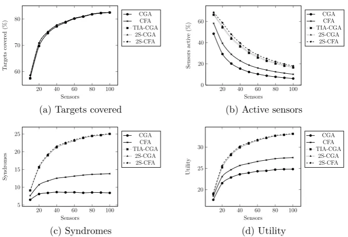
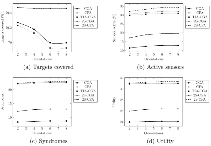
[image:38.595.109.491.134.249.2]

(39)

6.3.1 Number of sensors

For the first simulation set, we vary the number of sensors from 10-100 and

hold the number of targets constant at 50.

The results for the centralized algorithms are shown in Figure 4. As can

be seen in Figure 4a, as more sensors are added, the % of covered targets

increases, but the increase eventually slows down. All three heuristic

algo-rithms track CGA and CFA very closely. The diminishing increase in the

number of covered targets indicate that the system is becoming more and

more over-provisioned, with an increasing number of sensors becoming idle

since they no longer have any targets to cover or syndromes to contribute.

This is consistent with Figure 4b which shows the drop in % of sensors which

are active. Among the heuristic algorithms, 2S-CFA consistently utilizes

the most sensors, followed by 2S-CGA, and then TIA-CGA. In Figure 4c, we

see that consistent with their aims, all three heuristic algorithms consistently

have significantly higher number of syndromes than either CGA or CFA. The

number of syndromes increases with the number of sensors, but the increase

becomes more and more attenuated as the number of sensors increases. The

plateauing in the number of syndromes occurs much earlier for CGA and

CFA. The same pattern is seen in Figure 4d, which shows the system utility.

2S-CFA has a slight but consistent advantage over the other two heuristic

algorithms when it comes to the system utility garnered.

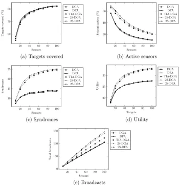
The results for the distributed algorithms are shown in Figure 5. As can

be seen in Figure 5a, as more sensors are added, the % of covered targets

(40)

20 40 60 80 100 60 70 80 Sensors T argets co v ered (%) CGA CFA TIA-CGA 2S-CGA 2S-CFA

(a) Targets covered

20 40 60 80 100 0 20 40 60 Sensors Sensors activ e (%) CGA CFA TIA-CGA 2S-CGA 2S-CFA

(b) Active sensors

20 40 60 80 100 5 10 15 20 25 Sensors Syndromes CGA CFA TIA-CGA 2S-CGA 2S-CFA (c) Syndromes

20 40 60 80 100 20 25 30 Sensors Utilit y CGA CFA TIA-CGA 2S-CGA 2S-CFA (d) Utility

Figure 4: Effect of varying the number of sensors on centralized algorithms.

α = 0.5, 50 targets, 50x50 space, 4 sensing orientations, sensing radius = 10.

are very similar for all algorithms, with TIA-DGA lagging just very slightly

behind the others. The plateauing indicates that the system is becoming

more and more over-provisioned, with more and more sensors becoming idle

since they no longer have any targets to cover or syndromes to contribute.

Consistent with this, Figure 5b shows the drop in % of active sensors. The

plots are quite similar for DGA and DFA, with the plots of the three

heuris-tic algorithms being higher - this is because TIA-DGA, DGA, and

2S-DFA utilize the additional sensors for increasing the number of syndromes.

Between the three heuristic algorithms, TIA-DGA utilizes a slightly lower

number of active sensors than the two 2-stage algorithms. In Figure 5c, we

see that consistent with their aims, TIA-DGA, 2S-DGA, and 2S-DFA

[image:40.595.122.476.123.364.2]

(41)

number of syndromes increases with the number of sensors, but the increase

becomes more and more attenuated as the number of sensors increases. The

number of syndromes plateaus much earlier for DGA and DFA. Between the

three distributed heuristic algorithms, and with respect to the number of

syn-dromes, 2S-DFA performs best, followed very closely by 2S-DGA, and then

TIA-DGA. The pattern for the number of syndromes is repeated for the

sys-tem utility (Figure 5d). As for the number of broadcasts made (Figure 5e),

all five algorithms follow a linear (increasing) relationship with the number

of sensors. The number of broadcasts for DGA and DFA are highly similar.

The slope for the TIA-DGA is slightly higher than that of DGA and DFA.

Both 2S-DGA and 2S-DFA have noticeably higher slopes than TIA-DGA,

with 2S-DFA having a slightly higher slope than 2S-DGA.

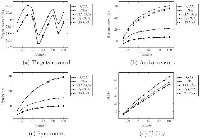
6.3.2 Number of targets

For the second simulation set, we vary the number of targets from 10-100

and hold the number of sensors constant at 50.

The results for the centralized algorithms are plotted in Figure 6.

Fig-ure 6a shows that the % of targets covered remains constant all throughout

the values tested (this means that the absolute number of targets covered

increases). As the number of targets increases, the % of sensors that are

active also increases (Figure 6b). We also see in Figure 6b that compared to

CGA and CFA, the three heuristic algorithms consistently have more

sen-sors that are active. Among the heuristic algorithms, 2S-CFA consistently

utilizes more sensors than 2S-CGA, which in turn, consistently utilizes more

(42)

heuris-20 40 60 80 100 60 70 80 Sensors T argets co v ered (%) DGA DFA TIA-DGA 2S-DGA 2S-DFA

(a) Targets covered

20 40 60 80 100 20 40 60 Sensors Sensors activ e (%) DGA DFA TIA-DGA 2S-DGA 2S-DFA

(b) Active sensors

20 40 60 80 100 10 15 20 25 Sensors Syndromes DGA DFA TIA-DGA 2S-DGA 2S-DFA (c) Syndromes

20 40 60 80 100 20 25 30 Targets Utilit y DGA DFA TIA-DGA 2S-DGA 2S-DFA (d) Utility

20 40 60 80 100 0 50 100 150 Sensors T otal broadcasts DGA DFA TIA-DGA 2S-DGA 2S-DFA (e) Broadcasts

Figure 5: Effect of varying the number of sensors on distributed algorithms.

α = 0.5, 50 targets, 50x50 space, 4 sensing orientations, sensing radius = 10.

tic algorithms consistently have more syndromes than CGA and CFA. The

same can also be said about the system utility, shown in Figure 6d. When

it comes to the system utility garnered, 2S-CFA once again has a slight but

consistent advantage over the two other heuristic algorithms.

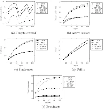
The results for the distributed algorithms are plotted in Figure 7.

Fig-ure 7a shows that the % of targets covered remains constant all throughout

[image:42.595.122.475.124.486.2]

(43)

20 40 60 80 100 78.2

78.4 78.6 78.8 79 79.2 79.4

Targets T argets co v ered (%) CGA CFA TIA-CGA 2S-CGA 2S-CFA

(a) Targets covered

20 40 60 80 100 10 20 30 40 Targets Sensors activ e (%) CGA CFA TIA-CGA 2S-CGA 2S-CFA

(b) Active sensors

20 40 60 80 100 10 20 30 Targets Syndromes CGA CFA TIA-CGA 2S-CGA 2S-CFA (c) Syndromes

20 40 60 80 100 10 20 30 40 50 Targets Utilit y CGA CFA TIA-CGA 2S-CGA 2S-CFA (d) Utility

Figure 6: Effect of varying the number of targets on centralized algorithms.

α = 0.5, 50x50 space, 50 sensors, 4 sensing orientations, sensing radius = 10.

(this means that the absolute number of targets covered increases). It can

also be seen in the plot that TIA-DGA trails the other four algorithms when it

comes to the % of targets covered. The number of active sensors increases for

all algorithms, although the increase is much steeper for TIA-DGA, 2S-DGA

and 2S-DFA than DGA or DFA (Figure 7b). The increase in the number

of active sensors can also be seen to plateau, as already active sensors prove

sufficient to cover the targets that are added. Between the three distributed

algorithms that are target-identifiability aware, the increase is greatest for

2S-DFA, followed by 2S-DGA, and finally, TIA-DGA. Consistent with the

algorithms’ aims, Figures 7c and 7d show that TIA-DGA, DGA and

2S-DFA consistently have more syndromes and higher system utilities than both

[image:43.595.122.476.126.368.2]