http://wrap.warwick.ac.uk
Original citation:
Thomason, Alasdair, Griffiths, Nathan and Sanchez Silva, Victor. (2015) Identifying
locations from geospatial trajectories. Journal of Computer and System Sciences.
doi: 10.1016/j.jcss.2015.10.005
Permanent WRAP url:
http://wrap.warwick.ac.uk/74011
Copyright and reuse:
The Warwick Research Archive Portal (WRAP) makes this work by researchers of the
University of Warwick available open access under the following conditions. Copyright ©
and all moral rights to the version of the paper presented here belong to the individual
author(s) and/or other copyright owners. To the extent reasonable and practicable the
material made available in WRAP has been checked for eligibility before being made
available.
Copies of full items can be used for personal research or study, educational, or
not-for-profit purposes without prior permission or charge. Provided that the authors, title and
full bibliographic details are credited, a hyperlink and/or URL is given for the original
metadata page and the content is not changed in any way.
Publisher’s statement:
© 2015, Elsevier. Licensed under the Creative Commons
Attribution-NonCommercial-NoDerivatives 4.0 International
http://creativecommons.org/licenses/by-nc-nd/4.0/
A note on versions:
The version presented here may differ from the published version or, version of record, if
you wish to cite this item you are advised to consult the publisher’s version. Please see
the ‘permanent WRAP url’ above for details on accessing the published version and note
that access may require a subscription.
Identifying Locations from Geospatial Trajectories
Alasdair Thomasona,∗, Nathan Griffithsa, Victor Sancheza
aDepartment of Computer Science, University of Warwick, Coventry, CV4 7AL, United Kingdom
Abstract
Harnessing the latent knowledge present in geospatial trajectories allows for the potential to revolutionise our understanding of behaviour. This paper discusses one component of such analysis, namely the extraction of significant locations. Specifically, we: (i) present the Gradient-based Visit Extractor (GVE) algorithm capable of extracting periods of low mobility from geospatial data, while maintaining resilience to noise, and addressing the drawbacks of existing techniques, (ii) provide a comprehensive analysis of the properties of these visits and consequent locations, extracted through clustering, and (iii) demonstrate the applicability of GVE to the problem of visit extraction with respect to representative use-cases.
Keywords: Geospatial, Location Extraction, Significant Locations, Trajectory, Visits
1. Introduction
The recent rise in the prevalence of location-aware hardware has brought with it an increase in the availability of geospatial trajectories, along with the consequent foundation for reasoning about the actions of users that this affords. Fundamentally, such trajectories are sets of spatio-temporal datapoints that relate the whereabouts of an individual, animal or other entity to specific times. The extraction of meaningful locations from geospatial data provides a basis for modelling a user’s interactions with their environment, an important part of many location-aware applications. Such applications may include location prediction, typically relying on extracted locations to discretise the set of possible predictive outcomes, or context-aware services such as recommender systems or digital assistants that use location to provide a greater level of personalisation.
This paper considers location extraction as a two-step process that first extracts periods of low mobility from geospatial data, referred to asvisits, and then clusters these visits together to formlocations. Specifi-cally, the paper provides a detailed discussion of existing techniques forvisit extractionandvisit clustering, and presents the Gradient-based Visit Extraction (GVE) algorithm for the purpose of visit extraction. This algorithm provides resilience to noise and overcomes several drawbacks of previous works: the algorithm does not place a minimum bound on visit duration, has no assumption of evenly spaced observations and operates in real-time without imposing a delay on trajectory points being considered. Additionally, we provide a thorough exploration of the parameter space for GVE through a comprehensive analysis of the properties of visits and locations produced, and demonstrate the applicability of GVE to the task of visit extraction with respect to representative use-cases and a comparison to the current state-of-the-art.
The remainder of this section discusses visit extraction and proposes two representative use-cases for extracted visits and locations. Section 2 discusses related work, including approaches to visit extraction and clustering. The GVE algorithm is presented and discussed in Section 3; discussion of the methodology employed to analyse the algorithm and the visits it produces can be found in Section 4. Finally, Section 5 details the results of the analysis and demonstrates the applicability of GVE to the task of visit extraction, with Section 6 providing a conclusion and summary of the findings and contributions made.
∗Corresponding author
Email addresses: [email protected](Alasdair Thomason),[email protected](Nathan Griffiths),
1.1. Visit Extraction
The extraction of locations meaningful to users is achieved by analysing the datapoints found within trajectories and identifying the regions where the user has spent time. Although a variety of techniques have been used in literature to extract locations from data, they are typically used as a precursor step to performing another activity, such as location prediction, and have not been investigated or evaluated in depth. While it is possible to perform location extraction by using a single clustering algorithm, the process is typically performed in two distinct clustering steps [1–3, 7, 24, 28]. The first step, visit extraction, is responsible for partitioning a temporally ordered dataset into periods of low mobility, referred to as either stops, stays or visits, where during each period the user is expected to have remained in one geographic location. For clarity, in this paper, we refer to such periods asvisits. Visits of no duration (i.e. either the visit consists of a single point, or all points that make up a visit were recorded at the same time instance) are classed as noise since they represent the user travelling and not being stationary. The second step in the process,visit clustering, summarises the extracted visits and performs clustering to determine which visits belong to the same location. Utilising a two-step approach for location extraction has several advantages, namely:
• Visit extraction can be performed in linear time, summarising vast portions of the dataset, thus reducing the complexity for the clustering step.
• By considering their temporal nature, individual data points that occur when an entity is moving are ignored. In traditional clustering, if several points were to be recorded in close proximity, but on different occasions, for instance along a road, an erroneous location would be identified.
• Extracted visits consist of contiguous points and thus characterise a period of time in which the user remained at the location, providing a basis for modelling historic time spent.
The disadvantages of the two-step process relate to the location clusters extracted at the visit clustering step. In order to reduce the complexity of this stage, extracted visits are typically summarised into a single point (e.g. centroid), and consequently the shape of overall locations extracted are not likely to be represented. Depending upon the goal of location clustering, this could be problematic.
1.2. Use-cases
The uses for extracted locations and visits are varied as they provide a foundation for modelling be-haviour. However, for the remainder of this paper we consider two representative examples, which apply equally well to trajectories from various sources. The first use-case, referred to asaccurate visits, considers the visits as a source of context, aiming to accurately characterise a user’s physical location at any point in time. In this case, clustered locations primarily serve to group the visits together to model transitions correctly. The second use-case,location properties, is less focused on visits, but rather, considers the accu-rate identification of the properties (i.e. shape and position) of locations. Accuaccu-rately identified locations are essential to certain services, such as creating geofences, where the visits are of less importance. It is impor-tant to note, however, that although thelocation properties use-case does not strictly require the accurate extraction of visits, the runtime of visit clustering algorithms is severely detrimented as the number of visits increases.
2. Related Work
selecting an appropriate value forkby performing the clustering multiple times on different parameters and observing the results. The particular algorithms employed here have their own respective drawbacks, and it is the focus of the remainder of this section to explore these drawbacks along with alternative approaches and related work. Towards understanding existing approaches to visit extraction and clustering, Section 2.1 begins with a discussion on the collection of data over which visit extraction can be performed. An overview of visit extraction techniques follows in Section 2.2, and visit clustering in Section 2.3. Finally, Section 2.4 explores work that has been conducted into enriching extracted locations with additional meaning and context information.
2.1. Data Collection
Before discussing methods of location extraction, it is important to consider the collection and processing of data, to gain an understanding of the properties expected when the location extraction stage is reached. In much existing research into location-aware systems, users are asked to carry battery-operated devices which record their location at predetermined intervals [3, 19, 24, 28, 31]. This approach places a burden upon the users who must ensure that the device remains with them and charged at all times. In part, these drawbacks have been reduced in recent years due to the inclusion of location-sensing hardware in personal smartphones, and thus recent location-aware literature has used data from such devices [7, 9, 18, 22, 24, 29]. Location is determined by the device through a combination of sensors, such as GPS, GLONASS and cell tower triangulation, where the accuracy of measurement is strongly correlated with the amount of power consumed.
Aiming to reduce the power overhead of data collection, Kiukkonen et al. present a state-based machine that transitions between different rates and location determination methods based on sensor readings [19]. Specifically, the authors use WiFi base stations to indicate locations when available, and adjust collection rate based on accelerometer readings (e.g. increasing collection rate when moving). Similarly, Chon et al. present an application, SmartDC, that aims to estimate when a user will leave a current area and increase collection around this time [10]. As a consequence of techniques such as this, and the limitations of these devices, it is important to note that the accuracy and rate of location collection will not remain constant.
2.2. Visit Extraction Techniques
Ashbrook and Starner’s approach, namely that of looking for periods of missing data within trajectories, is limited in that it assumes that all missing data is caused by a visit, and visits cannot occur when data was collected. Indeed, the authors note that the datalogging devices were prone to run out of battery power, also causing a lack of data. Building on this work, but assuming a constant flow of data, even when indoors, similar algorithms have been proposed. Relying on time and distance thresholds, the algorithms typically operate by iterating over a temporally ordered dataset and segmenting the data into visits, where no visit can be larger than a specified radius (or, sometimes, that no consecutive points can be greater than a specified distance apart) and the user must remain in this area for longer than a specified amount of time [1, 2, 17, 18, 28, 31, 33]. This approach was initially presented by Li et al., but has since been adapted for specific uses in literature [21]. Montoliu and Gatica-Perez also use this technique, but add an additional constraint that the time between consecutive data points in the same visit must be bounded [24]. This was proposed to prevent periods of missing data from being contained within a visit. If data became unavailable at one time, and became available at a nearby coordinate some time later, it is not possible to state with certainty that the user remained stationary for the missing period.
over a single small example, no quantitative evaluation of the properties of the visits extracted has been conducted.
In contrast to the approach of splitting a temporally ordered dataset into visits, there are methods of extracting visits that are not partitional in nature. ST-DBSCAN [8] and DJ-Cluster [32] are density-based clustering algorithms that are designed to cater for spatio-temporal data by extracting clusters that are similar in both space and time. While they overcome the problem of performing only two-dimensional clustering directly to trajectories (that of extracting dense groups of points without considering time), these approaches are computationally intensive, typically having runtimeO(n log n) as opposed to theO(n) of the other techniques discussed, and the resultant visits do not span continuous time periods.
Aiming to overcome the drawbacks of existing approaches, by assuming noise in the dataset, Bamis and Savvides present the STA extraction algorithm [6]. While the authors were specifically motivated by identifying activities that repeat in cycles through extraction and clustering, the first step, STA extraction, uses a definition of an activity that is identical to our definition of a visit, and thus performs visit extraction. The algorithm is similar to existing approaches in that it iterates over the trajectory points, but uses a weighted averaging filter to reduce the impact of noise before considering an activity as having ended. This technique however does bring with it several drawbacks and assumptions relating to the data, for example, requiring evenly time-sliced data and a full buffer before consideration of a visit can occur, consequently imposing a minimum bound on visit duration.
2.3. Visit Clustering
Extracted visits can be clustered together to form locations. Several general-purpose clustering tech-niques exist and have been used for this purpose, including k-means [3, 23] and DBSCAN [1, 5, 12, 24]. When clustering with k-means, the number of clusters to be extracted must be known a priori, which is not typical when extracting locations from trajectories. DBSCAN, on the other hand, has no such requirement, instead extracting clusters providing that a sufficient density of data points exist.
Focusing specifically on location extraction, Zheng et al. [28] propose a grid-based clustering algorithm that splits the considered area into uniform squares, where the size of each square is a user-specified pa-rameter. Squares that contain a greater number of visits than a threshold are then merged with all of their neighbours, providing that no dimension exceeds 3 squares in length. This requirement, although bounding location size, enforces the requirement for the maximum size of locations to be known a priori, and creates locations that are regular in shape. These locations may, therefore, not represent the shape of real-world locations accurately, and thus the algorithm is likely not applicable when considering thelocation properties use-case presented previously.
Finally, continuing on from their STA extraction algorithm, discussed in Section 2.2, Bamis and Savvides propose the STA clustering algorithm for the detection of activities that were performed in similar locations and at similar times of day. The STA clustering algorithm operates by summarising visits as their 3-dimensional bounding box (along the latitude, longitude and time dimensions) and progressively merging visits into clusters based on a similarity function, with weightings given to longitude, latitude and time. While it is possible to ignore the time dimension, as we would wish for location extraction, by setting the weighting to 0 the algorithm is not designed to merge all overlapping visits, only those whose dimensions are above a certain similarity, resulting in locations that can overlap. While the STA extraction algorithm is applicable for both extracting visits and activities, the STA clustering algorithm is not ideally suited to the task of visit clustering.
2.4. Enriching Locations
Once extracted, locations can be used as a basis for many location-aware systems and services, for example, to guide individuals around a city or other point of interest [27, 28, 30]. Further applications for extracted locations include categorising locations through supervised learning [1, 2, 11, 13], judging user similarity by location transitions [16], and the identification of activities from visited locations [5].
work in this area, using Markov models to model transitions between extracted locations [3, 4]. Building upon this, and considering time as well as the current location, Wang and Prabhala propose a combined transition and periodicity-based approach [26], and Fukano et al. investigate the use of a blockmodel to extract context from features collected from mobile phone logs, and use a scoring system on the extracted features to identify the likely next location [14]. Finally, in [15], Gao et al. investigate the reverse of the standard problem. Instead of taking a future time and asking where the user will be, they take a location and ask when the user will next visit, achieved by modelling the probability distribution of a user visiting each location for all possible times of day using Bayesian inference, and returning the time calculated to be most probable from historical information.
3. Gradient-based Visit Extractor
Adopting the two-step approach for location extraction, this section presents the Gradient-based Visit Extractor (GVE), which extracts visits from geospatial trajectories and addresses the drawbacks of existing approaches, making it capable of extracting visits from a wider variety of datasets. Section 2.2 discussed existing approaches to visit extraction, with the STA extraction algorithm identified as the current state-of-the-art [6]. Although an improvement on previous techniques, this algorithm has several limitations. Firstly, the algorithm assumes that the data occurs in even time slices. While some domains have regular and predictable data recording, for the purpose of extracting visits from data collected from devices carried by users, it is likely that conditions such as signal loss or lack of battery power would result in periods of time with varying collection rates, and periods with missing data entirely, thus resulting in non-evenly timesliced data. Secondly, the STA extraction algorithm requires that the buffer is full before consideration of a visit can occur, both imposing a delay on points being considered, as a sliding window of points is required for the weighted averaging filter to operate, and specifying a minimum bound on visit duration. The result of this is that the minimum visit length to be extracted must be known a priori and used to select appropriate parameters.
First described in [25], and presented in expanded form here with an additional consideration for handling large periods of missing data not present in the previous version, the Gradient-based Visit Extractor (GVE) algorithm is shown as Algorithm 1. The remainder of this section introduces and discusses the algorithm. In the following sections we demonstrate the applicability of GVE to the task of visit extraction, an evaluation lacking in previous work. Specifically, the evaluation performs a thorough exploration of the parameter space of the GVE algorithm and analyses properties of the visits extracted, through metrics discussed in Section 4, with results presented and discussed in Section 5. The evaluation continues with a comparison with the STA extraction algorithm and, through visit clustering with DBSCAN, discusses properties of the clustered locations, based on visits extracted from both the GVE and STA extraction algorithms. DBSCAN is selected due to its relevance to the domain and ability to extract clusters of arbitrary shape without the number of clusters being known a priori.
The Gradient-based Visit Extractor extracts visits from temporally-annotated geospatial trajectories by continually building a visit until adding another point would cause the recent trend of motion to be consistently away from the visit already extracted. Although similar in idea to STA, GVE can consider visits without having a full buffer of points over which to analyse the trend of motion and allows for points collected at a varying rate. Additionally, GVE is able to consider points as they arrive, while the STA extraction algorithm imposes a delay due to its method of averaging results over a window.
Algorithm 1Gradient-based Visit Extractor Algorithm
1: npoints, α, β, tmax//Input parameters
2: visits ←[ ]//Empty array, to be filled with visits
3: visit ←[p0 ]//Array containing the first point in the dataset 4: buffer ←[p0] //Buffer over which to consider trend of motion 5:
6: functionProcess(point) 7:
8: buffer.append(point)
9: if buffer.length> npoints then
10: buffer.shift
11: end if
12:
13: //A visit has ended if there is a significant amount of missing data or the user is moving away 14: if TimeBetween(visit.last,point)> tmax or MovingAway?(visit,buffer)then
15: if TimeBetween(visit.first,visit.last) >0then
16: visits.append(visit)//If the visit has some duration, store it
17: end if
18: visit ←[point] 19: buffer ←[point]
20: else
21: visit.append(point)//If the visit hasn’t ended, add the point to the visit
22: end if
23:
24: end function 25:
26: //The user is moving away from a visit if the gradient of the buffer is greater than the threshold 27: functionMovingAway?(visit,buffer)
28:
29: if Gradient(visit,buffer)>Threshold(α,β,buffer.length)then
30: returnTrue
31: else
32: returnFalse
33: end if
34:
temporal distances. Thegradient of bufferbis defined as:
Gradient(v,b) =
l(b)P
p∈b
(t(b, p)×d(v, p))−P
p∈b
t(b, p)P
p∈b d(v, p)
l(b)P
p∈b
t(b, p)2−(P
p∈b
t(b, p))2
wherel(b) is the current buffer size,t(b, p) is the temporal distance between the first point in the buffer and the current point,p, in seconds, andd(v, p) is the distance between pointpand the centroid of the current visit,v, in metres. A gradient greater than the threshold indicates that the visit has ended:
Threshold(α, β,length) =−log
length× 1
β
×α
With the gradient summarising the movement trend of the user relative to the visit, and a threshold function that returns a value dependent upon the number of points over which the gradient was calculated, we are now able to determine when a visit has ended: namely, if the gradient is greater than the threshold for a given set of points then the visit can be marked as having ended. This ensures resilience to noise by monitoring the movement trend over a set of points, but still allows for visits with few points.
In addition to trend of motion exceeding the threshold, a visit ends if the temporal distance between the point being considered and the immediately preceding point is greater than the parametertmax (line 14 of Algorithm 1), which is a similar technique to that used by Montoliu and Gatica-Perez to detect periods of missing data [24]. Without this consideration, if data were to be missing for several hours or days, but by chance the first point recorded after this period is geographically close to the last point recorded, the gradient would be extremely low and is likely to be below the threshold. In this instance, the point would be considered as part of the previous visit, even though a significant period of time had elapsed and the user could easily have left the visit and simply returned to a location nearby. By introducing a maximum time between consecutive points for them to be part of the same visit,tmax, we mitigate this issue. Conversely, two consecutive points that fall on the same time instance (i.e. there is no time between them), could cause a visit of no duration to be extracted. This is prevented in line 15 of Algorithm 1, where visits are only stored if they have a positive duration. A visit that consists of a single point, or a visit that consists of multiple points that fall on the same time instance would therefore be considered noise.
While parameter selection is dependent upon the specific application and dataset, we impose one primary constraint, namely β > npoints. If we permitted β to be less than npoints, it is possible for the threshold function to return a negative value when the size of the buffer exceedsβ. Using a negative threshold would allow a visit to be characterised as having ended when the gradient returns a negative value, where a negative gradient indicates that the user is moving towards the centre of the visit, rather than away from it. By requiringβ > npoints we ensure that any value returned by the threshold function is positive.
4. Experimental Setup
In order to demonstrate the applicability of the GVE algorithm to the problem of visit extraction, and to aid in parameter selection for future applications, we conduct a thorough analysis of the algorithm and resultant visits extracted. This analysis aims to guide application developers towards appropriate parameter choices, as well as demonstrating properties of the algorithm itself. Towards this goal, this section discusses the experimental methodology followed by presenting the algorithms and data selected for comparison, along with metrics through which analysis is conducted. The results of this exploration can be found in Section 5.
4.1. Algorithms
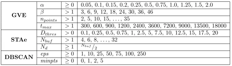
Table 1: Parameter sets for evaluation
GVE
α ≥0 0.05, 0.1, 0.15, 0.2, 0.25, 0.5, 0.75, 1.0, 1.25, 1.5, 2.0 β >1 3, 6, 9, 12, 18, 24, 30, 36, 46
npoints >1 2, 5, 10, 15, . . . , 35
tmax >1 300, 600, 900, 1200, 2400, 3600, 7200, 9000, 13500, 18000
STAe
Dthres >0 0.1, 0.25, 0.5, 0.75, 1, 2.5, 5, 7.5, 10, 12.5, 15, 17.5, 20 Nbuf >1 4, 6, 8, . . . , 32
Nd ≥1 Nbuf/2
DBSCAN eps ≥0 1, 10, 25, 50, 75, 100, 250
minpts ≥0 0, 1, 2, 5
While there are several approaches that have shown promise for this purpose, DBSCAN is widely used and has desirable properties, such as not requiring the number of locations to be known a priori [1, 5, 12, 24].
In order to ensure consistency, all implementations of the algorithms assume that distances are measured in metres, and time in seconds. Furthermore, we define the shape of a location to be the convex hull of the centroids of all visits belonging to the location. Summarising visits in such a way is an important part of the two-step approach to location extraction as it vastly reduces the complexity of the clustering procedure, and thus is a technique we employ here [1–3, 7, 24, 28].
4.2. Evaluation Parameters
With algorithms for evaluation selected, we narrow down the range of parameters considered. While it is not possible to consider all combinations of parameters, as many are unbounded, we select a range of parameters for each algorithm that aims to cover the parameter space as thoroughly as possible, ensuring that the results obtained are representative. The ranges of values selected for each parameter can be found in Table 1, and this section briefly discusses the parameters for each algorithm.
GVE takes 4 parameters: α and β alter the threshold function, where a gradient above the threshold indicates the end of a visit, withαscaling in they-dimension, andβ in thex-dimension. The npoints parameter specifies the maximum size of the buffer, andtmax specifies the maximum amount of time between two consecutive points permitted for the points to belong to the same visit. Only parameter combinations that obey the constraintβ > npoints are considered.
STA Extraction Algorithm has a fixed size buffer of lengthNbuf, and uses a weighted averaging function of window sizeNdto characterise the trend of motion, withDthres(measured in metres) specifying the threshold for the averaged buffers, above which the visit is considered to have ended. A relationship betweenNdandNbufwas proposed by the authors of the STA extraction algorithm, namelyNd= Nbuf
2 , and we adopt this approach here [6].
DBSCAN is a density-based clustering algorithm, whose two parameters,minptsandeps(), specify the required density of a cluster, with minptsspecifying the minimum number of points required within eps metres for a cluster to be extracted. A detailed explanation of how these parameters affect the extracted clusters can be found in [12].
4.3. Metrics
Selecting appropriate parameters for visit extraction and clustering is a difficult problem, not least because of the limited knowledge available relating to how altering parameters would affect the properties of the visits and locations produced. Adopting two application scenarios, namely the use-cases presented in Section 1.2, we explore the properties of visits and locations to gain a greater understanding of the applicability of certain algorithms and parameter sets.
This exploration is conducted with respect to metrics including the duration of visits extracted, pro-portion of data points classed as noise (as noise points indicate movement, this propro-portion is analogous to proportion of time spent travelling between locations), and the area of locations extracted. In these cases, while an application developer may not have specific target values, it is feasible that an acceptable range of values could be determined. As an example, if an application requires room-size locations, then average location area would be expected to be small, or if data were to be collected from a vehicle that is in motion for most of the day, noise proportion would be expected to be high.
4.3.1. Ground-truth Comparisons
Clustering is generally viewed as an unsupervised learning problem. In order to investigate how the results of clustering compare to an expected outcome, a ground-truth of visited locations needs to be available. If such a ground-truth exists, comparisons to the locations determined by the algorithms can be performed using the set-similarity measureDice’s coefficient:
QS= 2|A∩B|
|A|+|B|
where QS is the quotient of similarity in range [0,1]. A value of 1 indicates that the sets (A and B) are identical, while 0 indicates no overlap. Although Dice’s coefficient is designed for comparing the contents of two sets, it can be used over clusters by considering|A∩B|to represent the area covered by both clusters, and|A|+|B|to be the sum of the areas of the clusters, effectively providing a score for thelocation properties use-case.
4.4. Evaluation Data
4.4.1. Ground Truth Comparison Locations
The selection of distinct locations to use for comparison is extremely difficult in the absence of a ground truth provided by the users themselves. The MDC Dataset includes user-contributed places which are identified by algorithm and then labelled by the user. Unfortunately, this set is incomplete as it includes places for only a small proportion of the users in the dataset. Furthermore, manually overlaying the identified places on satellite imagery of the area provided no clear identification of the building or geographic feature to which the place belonged, as the corresponding points covered several buildings or landmarks. Instead of relying on these self-labelled places, we opt to identify manually 5 buildings or distinct geographic regions (e.g. a park) that were unambiguously visited for each user throughout the course of the data. This is achieved by overlaying all points belonging to a user on satellite imagery of the area, using Google Earth, and inspecting the resulting plots to identify dense areas of points that had a clear centre on a geographic feature or building. For each of the 9 users in our evaluation, we select 5 locations and summarise each location into a minimum set of points, which is stored for later comparison. Although this methodology is not flawless, as it may include locations visited a limited number of times, it provides an indication of how well the algorithms perform at extracting the geographical shape of visited locations as described in the location properties use-case in Section 1.2.
5. Parameter Exploration
Towards our goals of demonstrating the applicability of GVE to the task of visit extraction, and aiding in parameter selection for applications of the algorithm, this section presents the results observed from visit extraction under the methodology proposed in Section 4. This section begins with a parameter exploration of GVE, with results presented in Section 5.1, by analysing properties of the visits extracted with respect to the metrics discussed previously, then goes on to evaluate the locations extracted by clustering visits from both GVE and the STA extractor using DBSCAN (Sec. 5.2). Finally, Section 5.3 presents an evaluation of the applicability of both GVE and the STA extraction algorithm to the use-cases originally discussed in Section 1.2, when locations are determined by DBSCAN.
5.1. Gradient-based Visit Extractor (Visit Extraction)
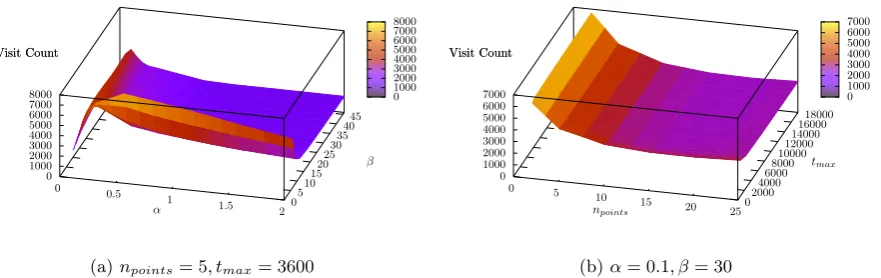
The effect of the parameters on the metrics discussed in Section 4.3 can be seen in Figures 1-3. In each figure, surface plots are shown with separate plots for parametersαand β and fornpoints and tmax, requiring the two missing parameters to be constrained. For supervised learning problems, it is possible that there would be optimal values that can be selected to achieve this goal. However, no such values exist for unsupervised clustering, so we opt for constraining parameters such that the resultant plots provide a representative view of the unconstrained parameters. Specifically, we opt forα= 0.1, β = 30, npoints = 5, tmax= 3600, which were empirically determined to provide a representative view of the trends present in the relationships between the parameter space and the metrics. It is important to note that these graphs are presented to show the trends, rather than specific values extracted. The specific values (e.g. number of visits extracted) vary considerably based on the dataset provided to the algorithm, while the trends remain constant.
05 10 1520 2530 3540 45 0
0.5 1
1.5 2 0 1000 2000 3000 4000 5000 6000 7000 8000 Visit Count β α Visit Count 0 1000 2000 3000 4000 5000 6000 7000 8000
(a)npoints= 5, tmax= 3600
02000 40006000 8000 1000012000 1400016000 18000 0 5 10 15 20 25 0 1000 2000 3000 4000 5000 6000 7000 Visit Count tmax npoints Visit Count 0 1000 2000 3000 4000 5000 6000 7000
[image:12.595.83.524.123.262.2](b)α= 0.1, β= 30
Figure 1: Parameter effect on the number of visits extracted
05 10 1520 2530 3540 45 0
0.5 1 1.5
2 0
0.2 0.4 0.6 0.8 1 Noise Proportion β α Noise Proportion 0 0.2 0.4 0.6 0.8 1
(a)npoints= 5, tmax= 3600
02000 40006000 8000 1000012000 14000 1600018000 0 5 10 15 20 25 0 0.2 0.4 0.6 0.8 1 Noise Proportion tmax npoints Noise Proportion 0 0.2 0.4 0.6 0.8 1
[image:12.595.78.518.306.448.2](b)α= 0.1, β= 30
Figure 2: Parameter effect on the proportion of points designated as noise
real-world visits will have been merged, causing a loss of information, thus invalidating the utility afforded by the start and end times of each visit.
When considering the number of visits extracted, the maximum time between consecutive points permit-ted for them to belong to the same visit,tmax, has limited impact as it affects very few visits (Figure 1b). With smalltmaxvalues, visits are split more frequently as smaller amounts of missing data cause a visit to be ended, thereby increasing the number of visits extracted. With larger values, the impact is no longer noticeable due to the relatively small number of periods of missing data in the dataset. However, setting tmax too large causes larger periods of missing data to be included within visits where it may have been possible for a user to leave the visit and return, reducing the accuracy of visit properties. Similarly,npoints is most impactful for small values. With a smallnpointsvalue, the gradient is calculated over a small number of samples only and is therefore more susceptible to noise, prematurely ending visits and causing the number of visits extracted to increase.
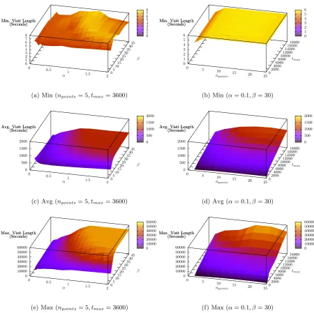
The relationships between the parameters and the number of visits extracted are corroborated by Fig-ures 3c and 3d, which show that when the number of visits extracted decreases, the average length of the extracted visits increases. While the maximum visit length (Figures 3e and 3f) also follows this general trend, it is important to note that low values ofαdo not have the same effect as with average visit length because the behaviour only affects very short visits.
05 1015 2025 30 3540 45
0 0.5
1 1.5 2 0 1 2 3 4 5 6 7 8
Min. Visit Length (Seconds)
β
α Min. Visit Length
(Seconds) 0 1 2 3 4 5 6 7 8
(a) Min (npoints= 5, tmax= 3600)
02000 4000 60008000 1000012000 1400016000 18000 0 5 10 15 20 25 0 1 2 3 4 5 6
Min. Visit Length (Seconds)
tmax
npoints
Min. Visit Length (Seconds) 0 1 2 3 4 5 6
(b) Min (α= 0.1, β= 30)
05 1015 2025 3035 40 45
0 0.5
1 1.5 2 0 500 1000 1500 2000
Avg. Visit Length (Seconds)
β
α Avg. Visit Length
(Seconds) 0 500 1000 1500 2000
(c) Avg (npoints= 5, tmax= 3600)
0 20004000 6000 800010000 1200014000 1600018000 0 5 10 15 20 25 0 500 1000 1500 2000
Avg. Visit Length (Seconds)
tmax
npoints
Avg. Visit Length (Seconds) 0 500 1000 1500 2000
(d) Avg (α= 0.1, β= 30)
05 1015 2025 3035 4045 0
0.5 1
1.5 2 0 10000 20000 30000 40000 50000 60000
Max. Visit Length (Seconds)
β
α Max. Visit Length
(Seconds) 0 10000 20000 30000 40000 50000 60000
(e) Max (npoints= 5, tmax= 3600)
02000 40006000 8000 1000012000 1400016000 18000 0 5 10 15 20 25 0 10000 20000 30000 40000 50000 60000
Max. Visit Length (Seconds)
tmax
npoints
Max. Visit Length (Seconds) 0 10000 20000 30000 40000 50000 60000
[image:13.595.70.521.192.641.2](f) Max (α= 0.1, β= 30)
Table 2: Parameter sets considered for GVE algorithm
ID α β npoints tmax Average Visit Count
GVE-1 0.25 12 10 1200 4914
[image:14.595.177.419.198.237.2]GVE-2 1.5 36 30 13500 1293
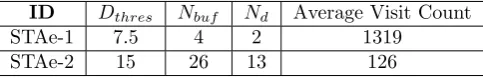
Table 3: Parameter sets considered for STA extraction algorithm
ID Dthres Nbuf Nd Average Visit Count
STAe-1 7.5 4 2 1319
STAe-2 15 26 13 126
does not impose a minimum bound on visit duration. While parameters may still influence the length of the shortest visit, with a large and varied dataset the effect of the parameters on minimum visit length is minimal. The results show that the shortest visit is extracted when bothαandβ are low, as this increases the likeliness of a visit being marked as having ended sooner. Additionally, lower values ofnpointscause the length of the shortest visit to decrease, as the algorithm is only considering the trend of motion over a small number of points. Not imposing a minimum bound on duration is beneficial because it allows arbitrarily short visits to be extracted, although in some cases this may not be desirable. If the dataset were collected at a very high rate, extremely short visits could be extracted. In certain applications these may not be required and so can be removed easily in a single step once visit clustering has completed by classifying the points belonging to them as noise retroactively.
5.2. DBSCAN (Visit Clustering)
With the properties of visits extracted through GVE better understood, the task now becomes clustering visits together to form locations. As detailed in Section 4.2, visit clustering is performed on sets of visits extracted using parameters selected to provide a representative overview of the relationship between the parameter space and characterisation metrics employed. Parameters have been selected for both the GVE and STA extraction algorithms for this purpose, and presented in Tables 2 and 3 respectively. Although a detailed analysis of the parameter space of the STA extraction algorithm is omitted for brevity, the number of visits extracted for all combinations of parameters was significantly lower than with GVE, making selection of sets of parameters that produced similar numbers of visits infeasible without constraining GVE’s parameters too heavily, and so only one set of parameters was selected for each algorithm that produced a similar number of visits (GVE-2 and STAe-1). Clustering was then performed on these extracted visits by DBSCAN with the parameters outlined in Section 4.2.
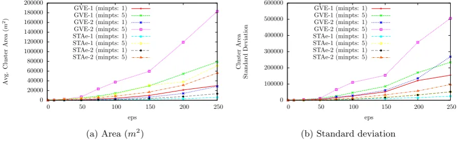
Figure 4 shows how the number of locations extracted varies with different algorithms and sets of pa-rameters for DBSCAN, for two different values ofminpts (1 and 5). The effect of theminpts parameter for DBSCAN is consistent and the remaining values not shown are omitted for brevity. The results show that DBSCAN performs predictably, and that the largest number of locations are extracted with the smallesteps andminptsparameters (i.e. requiring the lowest density of points to consider a location). Increasingminpts would require a higher density, thus creating fewer locations, and increasingeps would increase the area to consider for a location, thereby creating fewer, but larger, locations. This finding is reinforced by Figure 5, showing the average size of locations and the standard deviation of location sizes. The appropriate selection of parameters for clustering is important for both use-cases presented in Section 1.2. For accurate visits, locations are used to group visits together so that visits to the same location can be identified; therefore, locations that are too large or small will cause visits that are not to the same location to be grouped together incorrectly. The clustering step has a greater impact onlocation properties, however, as this use-case is solely interested in the clustered locations. Setting the parameters such that the locations extracted are too small will cause erroneous locations to be found as real-world locations are split into multiple parts, while if the extracted locations are too large, real-world locations will be merged.
0 500 1000 1500 2000 2500
0 50 100 150 200 250
Cluster
Coun
t
eps
[image:15.595.188.404.114.233.2]GVE-1 (minpts: 1) GVE-1 (minpts: 5) GVE-2 (minpts: 1) GVE-2 (minpts: 5) STAe-1 (minpts: 1) STAe-1 (minpts: 5) STAe-2 (minpts: 1) STAe-2 (minpts: 5)
Figure 4: Parameter effect on the number of locations extracted for DBSCAN
0 20000 40000 60000 80000 100000 120000 140000 160000 180000 200000
0 50 100 150 200 250
Avg. Cluster Area ( m 2) eps GVE-1 (minpts: 1) GVE-1 (minpts: 5) GVE-2 (minpts: 1) GVE-2 (minpts: 5) STAe-1 (minpts: 1) STAe-1 (minpts: 5) STAe-2 (minpts: 1) STAe-2 (minpts: 5)
(a) Area (m2)
0 100000 200000 300000 400000 500000 600000
0 50 100 150 200 250
Cluster
Area
Standard
Deviation
eps GVE-1 (minpts: 1) GVE-1 (minpts: 5) GVE-2 (minpts: 1) GVE-2 (minpts: 5) STAe-1 (minpts: 1) STAe-1 (minpts: 5) STAe-2 (minpts: 1) STAe-2 (minpts: 5)
(b) Standard deviation
Figure 5: Parameter effect on the average size of locations for DBSCAN
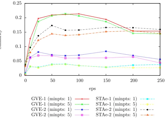
less straightforward. Figure 6 shows the relationship when calculating Dice’s coefficient for the location with the highest similarity to each ground truth location. Aseps is increased, the similarity begins to increase and then slowly falls back down as the value is increased further. Dice’s coefficient is maximal when the location and ground truth clusters are identical. If the extracted location is either larger or smaller than the ground truth, the similarity is lower. The results in Figure 6 show that, of the 4 sets of visits used as a basis for location clustering, GVE-1 (Table 2) produces locations that are closest to the ground truth.
5.3. Relation to Use-cases
Demonstrating the applicability of GVE to the problem of visit extraction, we focus on the two use-cases presented in Section 1.2. The first,accurate visits, is concerned with characterising where a user spent their time, achieved through the accurate identification of visits and subsequent accurate grouping together of visits to form locations. While it is not possible to state categorically the optimum parameters for achieving this goal for a given set of trajectories in absence of a concrete ground truth, we can use the exploration of the parameter space to reason about suitable ranges of parameters. Using knowledge about the source and length of trajectories, it would be reasonable to suggest an expected minimum number of visits, thereby allowing us to constrain the available parameter space. Furthermore, the expected ratio of time that a user spent travelling against time spent at a visit could be estimated, imposing minimum values for the proportion of noise in the trajectories, as the proportion of noise is approximately equivalent to proportion of time spent travelling between visits.
5.3.1. Accurate Visits
[image:15.595.72.524.272.410.2]0 0.05 0.1 0.15 0.2 0.25
0 50 100 150 200 250
Simiarit
y
eps
GVE-1 (minpts: 1) GVE-1 (minpts: 5) GVE-2 (minpts: 1) GVE-2 (minpts: 5)
[image:16.595.165.430.116.305.2]STAe-1 (minpts: 1) STAe-1 (minpts: 5) STAe-2 (minpts: 1) STAe-2 (minpts: 5)
Figure 6: Parameter effect on the similarity to ground truth for DBSCAN
• Users make an average of between 2 and 15 visits per day;
• The maximum length of a single visit does not exceed 2 days (172800 seconds);
• Each user made at least one short visit, for example to buy coffee or pay for a service, so the minimum visit duration must be less than 10 minutes (600 seconds);
• Each user spent at least 60% of their time at a visit location, and no more than 40% travelling between them (a noise proportion of less than 0.4).
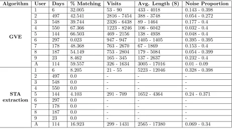
While it is true that these assumptions may not hold for every individual, for example it may be possible for a delivery driver to average more than 9.6 hours per day travelling (i.e. 40% of 24 hours), we believe they apply to the majority of people and, specifically, the majority of users who provided data for the MDC dataset. However, the assumption of maximum visit length is not as likely to hold with certain users if, for example, a hospital stay required them to remain stationary for more than 48 hours, or missing data occurred in the dataset and this was recorded as a visit by the STA extraction algorithm (GVE uses a parameter,tmax, to overcome this problem). We therefore investigate the effect of this set of assumptions with and without the assumption of maximum visit length. Using all sets of visits extracted with the parameters discussed in Section 4.2, we select only those that conform to these assumptions, with results shown in Tables 4 and 5 (with and without the maximum visit length assumption, respectively), listed per user, for both MDC users (represented by an ID number between 1 and 9) and the first author of this paper (represented byA). In both tables, the column titledMatching shows the percentage of parameter sets that produce visits consistent with the assumptions. It is important to note here that there are considerably more possible sets of parameters for GVE than the STA extraction algorithm (4290 and 195, respectively) as the GVE algorithm takes several more parameters and all combinations of parameters are considered. Despite there being more runs for GVE, both sets of parameters were selected to cover the parameter space as well as possible, and so the difference in the number of parameter sets should not have an impact on the results presented.
Table 4: Visit extraction summary (with maximum visit length assumption)
Algorithm User Days % Matching Visits Avg. Length (S) Noise Proportion
GVE
1 6 32.005 53 - 90 433 - 4018 0.143 - 0.398
2 497 42.541 2816 - 7454 388 - 3748 0.054 - 0.272
3 548 39.744 2326 - 6438 89 - 1464 0.177 - 0.4
4 550 67.366 1223 - 8246 106 - 6042 0.032 - 0.4
5 144 66.503 469 - 2156 138 - 4938 0.048 - 0.4
6 297 0.023 947 - 947 1405 - 1405 0.395 - 0.395
7 178 48.368 763 - 2670 67 - 1869 0.153 - 0.4
8 187 54.149 753 - 2804 179 - 5084 0.054 - 0.399
9 23 8.462 165 - 345 137 - 2637 0.232 - 0.4
A 114 59.557 326 - 1634 3005 - 17016 0.01 - 0.09
STA extraction
1 6 8.205 21 - 55 5223 - 12046 0.328 - 0.398
2 497 0.0 - -
-3 548 0.0 - -
-4 550 0.0 - -
-5 144 4.103 291 - 709 1652 - 4364 0.24 - 0.371
6 297 0.0 - -
-7 178 0.0 - -
-8 187 0.0 - -
-9 23 0.0 - -
-A 114 16.923 299 - 1431 2565 - 17380 0.069 - 0.34
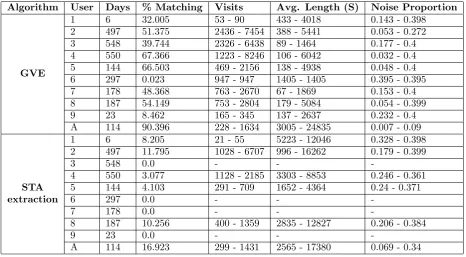
number of users for whom visits are extracted consistent with expectations is significantly reduced (3 out of 10 in Table 4, rising to 6 out of 10 when relaxing the maximum visit length assumption, shown in Table 5). Under these assumptions, therefore, it appears that GVE produces visits that are likely to be applicable to theaccurate visits use-case.
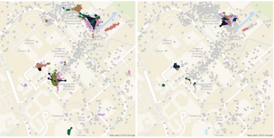
As discussed in Section 4.4, the licence for the MDC data prohibits the distribution of maps that may cause locations or users to be identified. For illustration, we therefore plot sample visits using trajectories from the first author of this paper, where the visits are from parameters that produce visit sets consistent with the assumptions outlined previously. Specifically, we select parameters by observing the results of plotting visits on a map and selecting only parameters that create visits consistent with the expectation that visits should not span multiple buildings. From this, the result with the lowest proportion of points designated as noise is selected for each algorithm. With visual observation confirming the correctness of visits, the visits with the lowest proportion of noise provide characterisation for the largest proportion of time. The plots are shown in Figure 7 and the properties of the visits listed in Table 6. In Figure 7, visits are represented by different colours with the convex hull of the points belonging to each visit illustrated in the same colour as the points. The convex hulls have been included for clarity so as to present which points belong to which visit unambiguously. In these specific cases, GVE has extracted several more, and shorter, visits than STA and also covers more of the trajectories, as demonstrated by a lower noise proportion, further indicating its applicability to the problem of visit extraction.
5.3.2. Location Properties
Table 5: Visit extraction summary (without maximum visit length assumption)
Algorithm User Days % Matching Visits Avg. Length (S) Noise Proportion
GVE
1 6 32.005 53 - 90 433 - 4018 0.143 - 0.398
2 497 51.375 2436 - 7454 388 - 5441 0.053 - 0.272
3 548 39.744 2326 - 6438 89 - 1464 0.177 - 0.4
4 550 67.366 1223 - 8246 106 - 6042 0.032 - 0.4
5 144 66.503 469 - 2156 138 - 4938 0.048 - 0.4
6 297 0.023 947 - 947 1405 - 1405 0.395 - 0.395
7 178 48.368 763 - 2670 67 - 1869 0.153 - 0.4
8 187 54.149 753 - 2804 179 - 5084 0.054 - 0.399
9 23 8.462 165 - 345 137 - 2637 0.232 - 0.4
A 114 90.396 228 - 1634 3005 - 24835 0.007 - 0.09
STA extraction
1 6 8.205 21 - 55 5223 - 12046 0.328 - 0.398
2 497 11.795 1028 - 6707 996 - 16262 0.179 - 0.399
3 548 0.0 - -
-4 550 3.077 1128 - 2185 3303 - 8853 0.246 - 0.361
5 144 4.103 291 - 709 1652 - 4364 0.24 - 0.371
6 297 0.0 - -
-7 178 0.0 - -
-8 187 10.256 400 - 1359 2835 - 12827 0.206 - 0.384
9 23 0.0 - -
-A 114 16.923 299 - 1431 2565 - 17380 0.069 - 0.34
Table 6: Metric summary of visualised visits
Visits Avg. Visit (s) Noise Proportion
GVE 695 7377 0.063
STA extraction 558 8991 0.118
(a) GVE (α= 0.05,β= 36,npoints= 5,tmax= 1200) (b) STA extraction (Dthres= 2.5,Nbuf = 6,Nd= 3)
Figure 7: Extracted visits
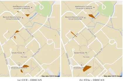
Table 7: Parameter summary of visualised clusters
Visit Clusterer Dice’s Coefficient minpts eps
GVE 0.28 2 25
Figure 8: Ground truth clusters
(a) GVE - DBSCAN (b) STAe - DBSCAN
[image:20.595.90.511.429.708.2]6. Conclusion
This paper has considered location extraction from geospatial trajectories as a two-step process. In the first step, periods of low mobility, referred to asvisits, are extracted from the data, with these visits then clustered into locations. Performing visit extraction as a precursor step, in such a manner, allows the summarisation of a large dataset into relatively few visits, drastically reducing the complexity of clustering. Once extracted, locations such as these are used as the basis for many applications and services, including location prediction and systems that utilise context in order to reason about users as both individuals and as groups.
The primary focus of this paper has been the presentation and analysis of GVE, the Gradient-based Visit Extractor algorithm, that extracts periods of low mobility from geospatial data while maintaining resilience to noise and overcoming the drawbacks of existing techniques. Specifically, GVE does not place a minimum bound on visit duration, has no assumption of evenly spaced observations and does not impose a delay on trajectory points being considered, making it amenable to visit extraction in real-time from a larger variety of data sources than existing approaches. In addition to presenting the algorithm, this paper has provided a comprehensive analysis of the properties of the visits extracted through an exploration of the parameter space, thus providing application developers with knowledge to aid in parameter selection. The applicability of GVE to the task of visit extraction was then demonstrated through both a comparison with the STA extraction algorithm, the current state-of-the-art, and analysis of locations determined through clustering with DBSCAN. In both of these investigations positive results demonstrating the suitability of GVE were achieved, with evidence indicating increased accuracy over existing approaches. This quantitative evaluation, lacking from previous work, demonstrates the applicability of the Gradient-based Visit Extractor (GVE) algorithm to the task of visit extraction and, consequently, as a precursor step to location extraction from geospatial trajectories.
7. Acknowledgements
Portions of the research in this paper used the MDC Database made available by Idiap Research Institute, Switzerland and owned by Nokia [19, 20].
References
[1] Gennady Andrienko, Natalia Andrienko, Georg Fuchs, Ana-Maria Olteanu Raimond, Juergen Symanzik, and Cezary Ziemlicki. Extracting Semantics of Individual Places from Movement Data by Analyzing Temporal Patterns of Visits. In
Proceedings of the ACM SIGSPATIAL International Conference on Advances in Geographic Information Systems, pages 5–8, Orlando, 2013.
[2] Gennady Andrienko, Natalia Andrienko, Christophe Hurter, Salvatore Rinzivillo, and Stefan Wrobel. From Movement Tracks Through Events to Places: Extracting and Characterizing Significant Places from Mobility Data. InProceedings of the IEEE Conference on Visual Analytics Science and Technology, pages 161–170, Providence, 2011.
[3] Daniel Ashbrook and Thad Starner. Learning Significant Locations and Predicting User Movement with GPS. In Pro-ceedings of the 6th International Symposium on Wearable Computers, pages 101–108, Seattle, 2002.
[4] Daniel Ashbrook and Thad Starner. Using GPS to Learn Significant Locations and Predict Movement Across Multiple Users.Personal and Ubiquitous Computing, 7(5):275–286, 2003.
[5] Roland Assam and Thomas Seidl. Context-based Location Clustering and Prediction using Conditional Random Fields. InProceedings of the 13th International Conference on Mobile and Ubiquitous Multimedia, pages 1–10, 2014.
[6] Athanasios Bamis and Andreas Savvides. Lightweight Extraction of Frequent Spatio-Temporal Activities from GPS Traces. InProceedings of the 31st Real-Time Systems Symposium, pages 281–291, San Diego, 2010.
[7] Athanasios Bamis and Andreas Savvides. Exploiting Human State Information to Improve GPS Sampling. InProceedings of the IEEE International Conference on Pervasive Computing and Communications Workshops, pages 32–37, Seattle, 2011.
[8] Derya Birant and Alp Kut. ST-DBSCAN: An Algorithm for Clustering Spatial–Temporal Data. Data & Knowledge Engineering, 60(1):208–221, 2007.
[10] Yohan Chon, Elmurod Talipov, Hyojeong Shin, and Hojung Cha. Mobility Prediction-based Smartphone Energy Opti-mization for Everyday Location Monitoring. InProceedings of the 17th International Conference on World Wide Web, pages 82–85, Seattle, 2011.
[11] Trinh Minh Tri Do and Daniel Gatica-Perez. The Places of Our Lives: Visiting Patterns and Automatic Labeling from Longitudinal Smartphone Data. IEEE Transactions on Mobile Computing, 13(3):638–648, 2013.
[12] Martin Ester, Hans-Peter Kriegel, J¨org Sander, and Xiaowei Xu. A Density-Based Algorithm for Discovering Clusters in Large Spatial Databases with Noise. InProceedings of the 16th International Conference on Knowledge Discovery and Data Mining, pages 226–231, Portland, 1996.
[13] Katayoun Farrahi and Daniel Gatica-Perez. Learning and Predicting Multimodal Daily Life Patterns from Cell Phones. InProceedings of the International Conference on Multimodal Interfaces, pages 277–280, Cambridge, 2009.
[14] Jun Fukano, Tomohiro Mashita, Takahiro Hara, Kiyoshi Kiyokawa, Haruo Takemura, and S Nishio. A Next Location Prediction Method for Smartphones Using Blockmodels. InProceedings of the IEEE Conference on Virtual Reality, pages 1–4, 2013.
[15] Huiji Gao, Jiliang Tang, and Huan Liu. Mobile Location Prediction in Spatio-Temporal Context.
[16] Yu Gong, Yong Li, Depeng Jin, Li Su, and Lieguang Zeng. A Location Prediction Scheme Based on Social Correlation. InProceedings of the IEEE Vehicular Technology Conference, pages 1–5, 2011.
[17] Ramaswamy Hariharan and Kentaro Toyama. Project Lachesis: Parsing and Modeling Location Histories. InProceedings of the 3rd International Conference on Geographic Information Science, pages 106–124, Adelphi, 2004.
[18] Jong Hee Kang, William Welbourne, Benjamin Stewart, and Gaetano Borriello. Extracting Places from Traces of Locations. InProceedings of the 2nd ACM International Workshop on Wireless Mobile Applications and Services on WLAN Hotspots, pages 110–118, Philadelphia, 2004.
[19] Niko Kiukkonen, Jan Blom, Olivier Dousse, Daniel Gatica-Perez, and Juha Laurila. Towards Rich Mobile Phone Datasets: Lausanne Data Collection Campaign. InProceedings of the First Workshop on Modeling and Retrieval of Context, 2010. [20] Juha K Laurila, Daniel Gatica-Perez, Imad Aad, Jan Blom, Olivier Bornet, Trinh Minh Tri Do, Olivier Dousse, Julien
Eberle, and Markus Miettinen. The Mobile Data Challenge: Big Data for Mobile Computing Research.
[21] Quannan Li, Yu Zheng, Xing Xie, Yukun Chen, Wenyu Liu, and Wei-Ying Ma. Mining User Similarity Based on Location History. InProceedings of the 16th ACM SIGSPATIAL International Conference on Advances in Geographic Information Systems, pages 34:1–34:10, Irvine, 2008.
[22] Lin Liao, Donald J Patterson, Dieter Fox, and Henry Kautz. Learning and Inferring Transportation Routines.Artificial Intelligence, 171(5-6):311–331, 2007.
[23] James MacQueen. Some Methods for Classification and Analysis of Multivariate Observations. InProcedings of the 5th Berkeley Symposium on Math, Statistics, and Probability, pages 281–297, Berkeley, 1967.
[24] Raul Montoliu and Daniel Gatica-Perez. Discovering Human Places of Interest from Multimodal Mobile Phone Data. In
Proceedings of the 13th International Conference on Mobile and Ubiquitous Multimedia, pages 12:1–12:10, Limassol, 2010. [25] Alasdair Thomason, Nathan Griffiths, and Matthew Leeke. Extracting Meaningful User Locations from Temporally Annotated Geospatial Data. InInternet of Things: IoT Infrastructures, volume 151 ofLNICST, pages 84–90. Springer, 2015.
[26] Jingjing Wang and Bhaskar Prabhala. Periodicity Based Next Place Prediction. InProceedings of the Nokia Mobile Data Challenge (MDC) Workshop in Conjunction with Pervasive, 2012.
[27] Vincent W Zheng, Bin Cao, Yu Zheng, Xing Xie, and Qiang Yang. Collaborative Filtering Meets Mobile Recommendation: A User-centered Approach. InProceedings of the 24th Conference on Artificial Intelligence, pages 236–241, Atlanta, 2010. [28] Vincent W Zheng, Yu Zheng, Xing Xie, and Qiang Yang. Collaborative Location and Activity Recommendations with GPS History Data. InProceedings of the 19th International Conference on World Wide Web, pages 1029–1038, Raleigh, 2010.
[29] Yu Zheng, Like Liu, Longhao Wang, and Xing Xie. Learning Transportation Mode from Raw GPS Data for Geographic Applications on the Web. In Proceedings of the 17th International Conference on World Wide Web, pages 247–256, Beijing, 2008.
[30] Yu Zheng, Xing Xie, and Wei-Ying Ma. GeoLife: A Collaborative Social Networking Service Among User, Location and Trajectory.IEEE Database Engineering Bulletin, 33(2):32–39, 2010.
[31] Yu Zheng, Lizhu Zhang, Xing Xie, and Wei-Ying Ma. Mining Interesting Locations and Travel Sequences from GPS Trajectories. InProceedings of the 18th International Conference on World Wide Web, pages 791–800, Madrid, 2009. [32] Changqing Zhou, Dan Frankowski, Pamela Ludford, Shashi Shekhar, and Loren Terveen. Discovering Personally
Mean-ingful Places: An Interactive Clustering Approach.ACM Transactions on Information Systems, 25(3), 2007.