A new contact detection algorithm for three dimensional non spherical particles

http://wrap.warwick.ac.uk/

Boon, C. W., Houlsby, G. T. and Utili, Stefano. (2013) A new contact detection algorithm for three-dimensional non-spherical particles. Powder Technology, 248. pp. 94-102. http://dx.doi.org/10.1016/j.powtec.2012.12.040

Permanent WRAP url:

http://wrap.warwick.ac.uk/71275

Copyright and reuse:

The Warwick Research Archive Portal (WRAP) makes this work of researchers of the University of Warwick available open access under the following conditions. Copyright © and all moral rights to the version of the paper presented here belong to the individual author(s) and/or other copyright owners. To the extent reasonable and practicable the material made available in WRAP has been checked for eligibility before being made available.

Copies of full items can be used for personal research or study, educational, or not-for-profit purposes without prior permission or charge. Provided that the authors, title and full bibliographic details are credited, a hyperlink and/or URL is given for the original metadata page and the content is not changed in any way.

Publisher statement:

© 2015 Elsevier, Licensed under the Creative Commons Attribution-NonCommercial-NoDerivatives 4.0 International http://creativecommons.org/licenses/by-nc-nd/4.0/

A note on versions:

The version presented here may differ from the published version or, version of record, if you wish to cite this item you are advised to consult the publisher’s version. Please see the ‘permanent WRAP url’ above for details on accessing the published version and note that access may require a subscription.

A NEW CONTACT DETECTION ALGORITHM FOR THREE-DIMENSIONAL NON-1

SPHERICAL PARTICLES 2

3

C.W. Boon1_{, G. T. Houlsby}1 _{and S. Utili}2 4

1_{Department of Engineering Science, Oxford University Parks Road, Oxford OX1 3PJ,} 5

United Kingdom 6

2_{School of Engineering, University of Warwick, Coventry CV4 7AL, United Kingdom;} 7

formerly at University of Oxford. 8

9

ABSTRACT 10

A new contact detection algorithm between three-dimensional non-spherical particles in 11

the discrete element method (DEM) is proposed. Houlsby previously proposed the concept 12

of potential particles where an arbitrarily shaped convex particle can be defined using a 2nd 13

degree polynomial function [1]. The equations in 2-D has been presented and solved using 14

the Newton-Raphson method. Here the necessary mathematics is presented for the 3-D 15

case, which involves non-trivial extensions from 2-D. The polynomial structure of the 16

equations is exploited so that they are second-order cone representable. Second order-cone 17

programs have been established to be theoretically and practically tractable, and can be 18

solved efficiently using primal-dual interior-point methods [13]. Several examples are 19

included in this paper to illustrate the capability of the algorithm for particles of various 20

shapes. 21

22

Keywords: DEM; non-spherical; polyhedral; contact detection; potential particles; 23

NOTATIONS 25

a, b, c, d constants defining a plane in 3D 26

f mathematical function defining a potential particle 27

k fraction of the spherical term of a potential particle, and when subscripted 28

represents that thecoefficients with k has been factored out 29

pi slack variables for the planar terms of a potential particle

30

q unit quaternion

31

Q rotation matrix

32

r radius of the curvature at the edges of a potential function without the 33

spherical term 34

R radius of the spherical part of the particle 35

s slack variable for a potential function 36

x, y, z Cartesian coordinates 37

x vector of Cartesian coordinates

38

w constants for slack variables 39

θ particle orientation 40

A subscript identifying particle A 41

B subscript identifying particle B 42

43

44

1 INTRODUCTION 45

46

Although spheres remain popular in the discrete element method (DEM) because of their 47

computational efficiency in contact detection, particles in real life are largely non-48

spherical. Granular and powder materials are present in many shapes, most of which are 49

applications. These encompass operations such as storage, conveying, mixing and sizing 51

from small scale pharmaceutical or food processing operations, where composition control 52

may be critical, to large scale industry storage where wall stresses may be important. Non-53

spherical granular particles, e.g. tablets, are frequently encountered in the chemical, food 54

and pharmaceutical industries. The flow, arching and jamming mechanisms of these 55

particles in hoppers and silos are more complex than for spherical particles. For instance, 56

Cleary & Sawley [8] showed that the effect of particle shape on hopper discharge and 57

stress patterns can be significant. Wu & Cocks [19] and Mack et al. [20] have compared 58

the results of DEM simulations with real experimental data in 2-D and 3-D respectively. 59

They showed that particle shapes can significantly influence the particle flow properties. 60

61

Various methods to model non-spherical particles have been proposed in the literature, 62

most of which impose restrictions on the shape of the particles, i.e., either the particle has 63

to be polyhedral or the particle shape is restricted to a particular type of function [2, 3, 4, 5, 64

6, 7, 9]. In applications such as powder technology, where particles may assume a wide 65

range of shapes, it is important to have a 3-D contact detection algorithm that is as general 66

as possible so that the same algorithm can be used repeatedly for different processes. This 67

also allows numerical parametric studies to be performed across different particle shapes 68

without being limited by the capability of the contact detection algorithm that has been 69

implemented into the DEM code. The method of potential particles introduced by Houlsby 70

[1] can model any convex particle shape from circular to roughly polygonal in 2-D and 71

from spherical to roughly polyhedral in 3-D. In his paper, the contact detection algorithm 72

in 2-D has been presented and solved using the Newton-Raphson method. Here, the 73

solution for the 3-D case, which involves some non-trivial extensions from 2-D, is 74

(SOCP), which has been widely established to be theoretically and practically tractable. 76

SOCP solvers are generally held to be robust and efficient because they can use primal-77

dual interior-point methods. 78

79

In the next section, the mathematical formulation of the proposed contact detection 80

algorithm is illustrated. In the following section, three numerical examples are provided to 81

illustrate the capabilities of the algorithm for non-spherical particles of different shapes. 82

The robustness of the algorithm was tested for particles of both low and high aspect ratios. 83

84

85

2 THEORY AND METHODOLOGY 86

2.1 Particle Definition 87

88

Based on the notion that a convex particle can be constructed from an assembly of lines in 89

2-D or planes in 3-D, Houlsby [1] describes an arbitrary convex particle in terms of a 2nd 90

degree polynomial function (with respect to a local coordinate system). In 3-D, it can be 91

expressed as: 92

(1 ) ( 2 2 2 2)

1

2 2

R z y x k r d z c y b x a k

f N

i

i i i

i ⎟+ + + −

⎠ ⎞ ⎜

⎝

⎛ _{+ + − −}

−

=

∑

=

(1) 93

where (ai, bi, ci) is the normal vector of the ith plane defined with respect to the particle

94

local coordinate system, and di is the distance of the plane to the local origin. 〈 〉 are

95

Macaulay brackets, i.e., 〈x〉 = x for x > 0; 〈x〉 = 0 for x≤ 0. The planes are assembled such 96

that their normal vectors point outwards. They are summed quadratically and expanded by 97

a distance r (see Figure 1(a)), which is also related to the radius of the curvature at the 98

with 0 < k ≤ 1 denoting the fraction of sphericity of the particle (see Figure 1(b), (c) and 100

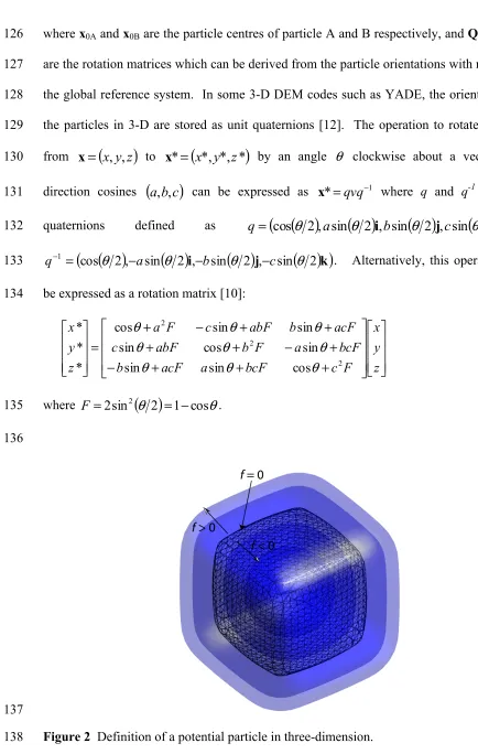
(d)). Houlsby [1] calls this function a “potential particle”, which has the following 101

properties (see Figure 2): 102

• f = 0 defines the particle surface, 103

• f < 0“inside” the particle, 104

• f > 0 “outside” the particle, 105

• the particle is strictly convex, and any surface f=constant is strictly convex. 106

For computational reasons, the expression in Eq. (1) is normalised (slightly changing the 107

meaning of k): 108

⎟⎟⎠ ⎞ ⎜⎜⎝

⎛ _{+ + −}

+

⎟ ⎟ ⎠ ⎞ ⎜

⎜ ⎝ ⎛

− −

+ +

−

=

∑

=

1 1

) 1

( 2_{2 2}2 2₂

1 2

2

R z R

y R

x k r

d z c y b x a k

f N

i

i i i i

(2)

109

110

111

(a) (b)

After  adding   spherical  term Before  adding  

spherical  term

(c)

Before  adding  

spherical  term After  adding  spherical  term

(d)

Before  adding   spherical  term

After  adding   spherical  term

113

Figure 1 Construction of potential particles (a) constituent planes are squared and 114

expanded by a constant r. A fraction of sphere is added. Particles with the spherical term 115

are visible in (b) k = 0.9, (c) k =0.7, (d) k = 0.4 116

117

118

2.2 Transforming the Reference System 119

Consider two potential particles, particle A fA(xA, yA, zA) = 0 and particle B fB(xB, yB, zB) = 120

0 defined in their local coordinates (xA, yA, zA) and (xB, yB, zB) respectively. For the 121

purpose of contact detection between a pair of particles, it is necessary to work with the 122

positions and orientations of the particles with respect to the same global coordinate 123

system. A point x in the global coordinate system can be calculated from the local 124

coordinate system xA or xB using the following expression: 125

x Q x= _{A A}+x0_A

⎪⎭ ⎪ ⎬ ⎫

where x0A and x0B are the particle centres of particle A and B respectively, and QA and QB 126

are the rotation matrices which can be derived from the particle orientations with respect to 127

the global reference system. In some 3-D DEM codes such as YADE, the orientations of 128

the particles in 3-D are stored as unit quaternions [12]. The operation to rotate a vector 129

from x=

(

)

(

)

direction cosines

(

)

131

quaternions defined as q=

(

( )

θ

( )

θ

( )

θ

( )

θ

)

( )

( )

( )

( )

(

)

1 _{θ a θ b θ c θ}

q− = − − − _{. Alternatively, this operation can}

133

be expressed as a rotation matrix [10]: 134 ⎥ ⎥ ⎥ ⎦ ⎤ ⎢ ⎢ ⎢ ⎣ ⎡ ⎥ ⎥ ⎥ ⎦ ⎤ ⎢ ⎢ ⎢ ⎣ ⎡ + + + − + − + + + + − + = ⎥ ⎥ ⎥ ⎦ ⎤ ⎢ ⎢ ⎢ ⎣ ⎡ z y x F c bcF a acF b bcF a F b abF c acF b abF c F a z y x 2 2 2 cos sin sin sin cos sin sin sin cos * * * θ θ θ θ θ θ θ θ θ (4)

where _{F =}2sin2

( )

. 135

136

137

Figure 2 Definition of a potential particle in three-dimension. 138

140

2.3 Contact Detection Algorithm 141

To perform contact detection between a pair of potential particles fA and fB, Houlsby [1] 142

proposes that one can solve one of the constrained minimisation problems below: 143

• minimise fA subject to the constraint fB = 0 144

• minimise fA+ fB subject to the constraint fA – fB= 0 145

Here, the second method is adopted, which corresponds to finding a point which is midway 146

and closest to both (with respect to the potential functions of the particles). It is 147

noteworthy that the presence of Macaulay brackets in Eq. (1) results in a discontinuity in 148

the second derivatives which can cause convergence issues in the process of optimisation. 149

Harkness [11] later suggested that the terms consisting of the Macaulay brackets can be 150

raised to a 3rd degree. However, the result of formulating the optimisation problem into a 151

second-order cone program (SOCP) makes this step unnecessary. The ith term in the 152

Macaulay brackets are each replaced with slack variables pi and inequality constraints:

153

a_ix+b_iy+c_iz−d_i ≤ p_i

⎭ ⎬ ⎫

(5) pi ≥0

After some algebraic manipulations (see Appendix A), the second-order cone program can 154

be formulated as follows: 155

minimise sA+sB

⎪ ⎪ ⎪ ⎪ ⎪ ⎪ ⎪ ⎪ ⎪ ⎪ ⎪ ⎪ ⎪ ⎪ ⎪ ⎪ ⎪ ⎪ ⎪ ⎪ ⎪ ⎪ ⎭ ⎪ ⎪ ⎪ ⎪ ⎪ ⎪ ⎪ ⎪ ⎪ ⎪ ⎪ ⎪ ⎪ ⎪ ⎪ ⎪ ⎪ ⎪ ⎪ ⎪ ⎪ ⎪ ⎬ ⎫ (6) subject to

Ak2 Ak2 Ak2 A

1 2 Ak A s z y x p N i

i + + + ≤

∑

i + + + ≤

s_A =s_B

(

)

Asx Q w y Q w z Q w x Q w y Q w z Q x x

w + + − + + = −

(

)

23 A Ak As 22 A Ak As 21 A Ak

Asx Q w y Q w z Q w x Q w y Q w z Q y y

w + + − + + = −

(

)

Asx Q w y Q w z Q w x Q w y Q w z Q z z

w + + − + + = −

w_Asa_iAx_Ak+w_Asb_iAy_Ak+w_Akc_iAz_Ak−w_App_iAk ≤d_iA, i =1,...,N_A,

wBsaiBxBk+wBsbiByBk+wBkciBzBk−wBppiBk≤diB, i=1,...,NB,

s_A ≥0

s_B ≥0

156 where: 157 A A Ap 1 k r w − = ⎪ ⎪ ⎪ ⎪ ⎪ ⎪ ⎪ ⎭ ⎪⎪ ⎪ ⎪ ⎪ ⎪ ⎪ ⎬ ⎫ (7) A A As k R w = B B Bp 1 k r w − = B B Bs k R w =

Note that the variables with subscript k are related to the original variables in Eq. (2), (3), 158

(4) and (5) through: 159 _A A A Ak 1 i

i _r p

k p = −

⎪ ⎪ ⎪ ⎪ ⎪ ⎪ ⎪ ⎭ ⎪⎪ ⎪ ⎪ ⎪ ⎪ ⎪ ⎬ ⎫ (8) _A A A

Ak _R x

_A

A A Ak _R y

k y =

_A

A A

Ak z

R k z =

160

Eq. (6) can be input directly into second-order cone optimisers such as MOSEK [14]. 161

There is overlap if both sA < 1.0 and sB < 1.0. Notice that a linear inequality is introduced 162

for every plane “i”. If there is overlap, the optimal point (xAk*, yAk*, zAk*) has to be 163

transformed back to the original local coordinates of particle A (xA*, yA*, zA*) using Eq. (8). 164

Thereafter, one can find the global Cartesian coordinates using Eq. (4). This point is then 165

used as the contact point, i.e, the point at which contact forces are applied between two 166

particles. 167

168

169

2.4 Calculating the Contact Normal 170

For particles of equal stiffness, the unit vector identifying the direction of the plane of 171

contact (i.e. the normal to the plane) can be calculated as the average between the two unit 172

normal vectors of the two interacting particles. The contact normal can be assigned as a 173

weighted average of the normal vectors of the interacting particles at the contact point 174

based on the particle stiffnesses. For each particle, the normal vector has been calculated 175

at the point of contact with the other particle. In local coordinates, the normal vector of a 176

particle can be calculated as: 177

⎟⎟⎠ ⎞ ⎜⎜⎝

⎛

∂ ∂ ∂ ∂ ∂ ∂

=

∇

z f y f x f

f , , (6)

x R k d z c y b x a a r k x f i i i i i i 2 N 1 2 2 ) 1 (

2 − _{+ + − +}

= ∂ ∂

_∑

_∑

_∑

The normal vector can be transformed into global coordinates using Eq.(4). The overlap 179

distance can be found by performing a line search along the contact normal and bracketing 180

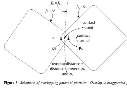
two points, i.e., one on particle A (fA = 0) and the other on particle B (fB = 0) (see Figure 181

3). The overlap distance is the distance between these two points. 182

183

184

Figure 3 Schematic of overlapping potential particles. Overlap is exaggerated for the 185

purpose of illustration. 2-D polygons are plotted for sake of explanation. 186

187

188

To illustrate the capability and robustness of the proposed contact detection algorithm, 190

some example simulations were run using the open-source discrete element code YADE 191

[12]. The second-order cone program (SOCP) was solved using the conic optimiser 192

MOSEK [13, 14]. For every potential contact, MOSEK was called as an external library in 193

a routine in YADE, by specifying inputs which consists of the objective function and 194

constraints. The solution calculated by MOSEK was then used as the contact point. 195

196

197

3.1 TEST A 198

199

In the first simulation, 360 cubes were generated with random orientations. Subsequently, 200

they were allowed to fall under gravity impacting the base of a prismatic container (see 201

Figure 4(a)). All the particles were assumed to be frictionless. In this example, a 202

combination of several contact conditions, involving angular corners, angular edges and 203

roughly flat surfaces is present throughout the simulation so that the robustness of the 204

algorithm can be tested. Once the cubes have settled (Figure 4(b)), an orifice at the base of 205

the container was opened (Figure 4(c)). The size of the orifice was 3 × 3 times the edge 206

length of the cubes, while the size of the base was 9 × 9 times the edge length of the cubes. 207

The simulation was repeated with tetrahedral particles (see Figure 5), whose size was 208

chosen as to be tightly inscribed in the cubes. The volume of these tetrahedra is one-third 209

that of the circumscribing cubes, and their edge length is 2 times the length of the cubes. 210

The adopted contact law in the normal direction is linear elasticity (elastic spring acting 211

only in compression) whereas in the shear direction is linearly elastic-perfectly plastic 212

(elastic spring plus a frictional slider). The contact stiffness in both directions has been 213

particles was scaled to 10000 kg/m3. The density of the tetrahedron was assumed to be 3 215

times the cube density so that they have the same mass. Table 1 summarises the 216

parameters used in this test. The flow of the particles over time is shown in Figure 6. The 217

simulation correctly shows that the flow rates of particles through an orifice are influenced 218

by their shapes; an inaccurate algorithm is likely to have resulted in similar flow rates 219

between shapes if the same particle size is modelled. The difference between the 220

deposition levels after settling (before the orifice is opened) is also captured realistically by 221

the contact detection algorithm (see Figure 4 (b) and Figure 5 (b)); note that the volume 222

ratio for a tetrahedron inscribed in a cube is 1:3. 223

224

TABLE 1: Parameters for Test A 225

Parameters Values

Density 10000 kg/m3

Normal stiffness 1 GN/m

Shear stiffness 1 GN/m

Friction angle of particles and containers 0°

Container dimension 9 m × 9 m × 14 m

Orifice dimension 3 m × 3m

Cube dimension 1 m × 1m × 1 m

226

(a) (b) (c) 228

Figure 4 Simulations of cube-shaped particles (a) filling the container (b) settling and (c) 229

flowing through the orifice 230

231

232

(a) (b) (c)

Figure 5 Simulations of tetrahedral-shaped particles (a) filling the container (b) settling 234

and (c) flowing through the orifice 235

236

237

238

0

50 100 150 200

250

300 350 400

0 50 100 150 200 250

Num

b

er

of

p

ar

tic

les

p

assi

n

g

the

or

if

ice

Time (s)

cube

tetrahedron

239

Figure 6 Discharge flow of particles through the orifice over time. It should be noted that 240

t=0 in this figure is the time when the orifice is opened, not the start of the simulation 241

242

243

244

3.3 TEST B 245

246

In this test, simulations were carried out using frictionless particles of high aspect ratios. 247

In the first test, the prisms have aspect ratios of 1:3. In the second test, the prisms have 248

aspect ratios of 1:8. First, like in Test A, the particles were generated with random 249

density and contact stiffness of the particles were the same as in Test A. Figure 7 (a) and 251

Figure 8 (a) show the particles falling under gravity and dynamically re-orienting 252

themselves in the container. Figure 7 (b) and Figure 8 (b) show the configurations of the 253

particles after they have settled. These particles re-aligned nicely with the container, 254

showing that the algorithm is able to model particles of high aspect ratios realistically. The 255

results conform to physical experience. 256

257

(a) (b)

258

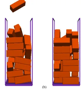
Figure 7 Simulations of prisms of aspect ratio 1:3 (a) filling the container and dynamically 259

changing positions (b) after settling. Some particles are leaning against the front wall of 260

the container (transparent in this figure). The accuracy of the figure is limited by the size 261

of tessellations of the visualisation tool. 262

(a) (b) 264

265

Figure 8 Simulations of prisms of aspect ratio 1:8 (a) filling the container and dynamically 266

changing positions (b) after settling. Some particles are leaning against the front wall of 267

the container (transparent in this figure). The accuracy of the figure is limited by the size 268

of tessellations of the visualisation tool. 269

270

271

272

273

3.3 TEST C 274

275

The conic optimisation formulation in Eq. (6) can be solved using a variety of numerical 276

techniques. The computation time for contact detection depends on the details of the 277

numerical technique used to solve the optimisation problem. From our experience, primal-278

robust, e.g. MOSEK [14] and CPLEX [15]. But the same formulation can be solved using 280

other general non-linear optimisation software [18]. The choice of the optimisation 281

software depends on its compatibility with the DEM code in terms of programming 282

language, operating system, cost of the licence and compiler version restrictions. 283

284

The computation time also depends on the termination criteria that are set for the 285

optimisation task. Most well-developed optimisation softwares make use of more than two 286

termination criteria and offer a range of “refinement” parameters. These termination 287

criteria and “refinement” parameters are normally different between optimisation softwares 288

since different optimisation techniques are used. Values for the termination criteria are set 289

based on the accuracy desired by the users. Note, however, that even considering the same 290

software, the numerical values of the termination criteria are not universal because certain 291

particle shapes may be more sensitive to the criteria than others. 292

293

For quasi-static problems, the contact point for a pair of particles in contact may be very 294

close to the contact point in the previous time step. With a good starting point, warm-295

starting allows the solver to take less Newton steps to satisfy the same termination criteria. 296

It is worth noting that although primal-dual interior point methods are preferred in the 297

optimisation literature to solve second-order cone programs because of their efficiency and 298

robustness, they do not allow warm-starting, i.e. they cannot make use of user-supplied 299

starting point information. If the modeller wishes to warm-start, the conventional primal 300

barrier method can be used to solve the second-order cone program [16]. Depending on 301

the experience of the modeller, he may wish to program his own Newton method for the 302

optimisation problem to allow more flexibility in fine-tuning the parameters for the solver, 303

point strategies. Another convenient way to warm-start is to use general non-linear 305

optimisation softwares which can make use of user-supplied starting point information. 306

Since different solvers (or strategies) may have different performances in terms of speed 307

and robustness, it is recommended that more than one solver is employed in the DEM code 308

of interest. Different solvers can be called under different circumstances, depending on the 309

strategy of the modeller. The fine-tuning strategies usually relate to the experience of the 310

modeller. In general, the computation time increases with the strictness of the termination 311

criteria (normally at the expenses of accuracy) and reduces with the “tuning” 312

aggressiveness (normally at the expenses of robustness). The overall run-time of a DEM 313

calculation further depends on the type of simulation and its parameters which are likely to 314

affect the number of “fortuitous encounters” of good starting points. It is also affected 315

inherently by the particle shape; certain shapes experience higher coordination numbers 316

(number of contacts per particle) and certain shapes can be more efficiently inscribed 317

inside axes-aligned bounding boxes or spheres which are used before the actual contact 318

resolution stage. 319

320

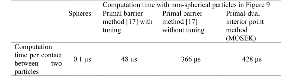
As an example, we show the computation time to solve Eq. (6) for a pair of particles in 321

contact (see Figure 9) using MOSEK and the primal barrier method code which can be 322

downloaded from [17]. In the primal barrier solver, we have substituted the equality 323

constraints into the objective and constraint functions (refer to Eq. (6)) so that the 324

equations are solved in terms of global coordinates rather than using two sets of local 325

coordinates. Note that the formulation in Eq. (6) is proposed here because it is accepted by 326

the majority of conic or non-linear optimisation solvers; certain conic optimisation 327

software may impose restrictions on the mathematical expressions of the second-order 328

used the primal barrier method for contact detection. These particles were fixed in space. 330

Using one of the two cores of the Intel Core 2 Duo processor, the computation time for the 331

barrier method with warm-starting was 366 µs; default values in [17] for the penalty 332

increment parameter and termination criteria were used. Using a more aggressive penalty 333

parameter with the same termination criteria, the computation time was 48 µs. In these two 334

barrier calculations, we have used the contact point calculated at the previous time-step as 335

the starting point. At the starting point, we have chosen the slack variables s’s and p’s in 336

Eq. (6) such that the inequalities are satisfied to within a margin of 10-5. Using exact 337

values without perturbation may cause numerical difficulties since the inequalities are 338

modelled inside log functions in the barrier method. These implementation details will 339

vary with the type of numerical technique. The computation time for MOSEK using its 340

default termination criterion was 428 µs. Table 2 shows the results of this exercise. 341

342

343

TABLE 2: Computation time comparison between choices of solvers 344

Computation time with non-spherical particles in Figure 9 Spheres Primal barrier

method [17] with tuning

Primal barrier method [17] without tuning

Primal-dual interior point method (MOSEK) Computation

time per contact

between two

particles

0.1 µs 48 µs 366 µs 428 µs

345

347

Figure 9 Two rounded tetrahedral particles in contact 348

349

350

4 CONCLUSIONS 351

The mathematics for the contact detection between potential particles in 3-D is presented. 352

The optimisation problem was cast into a second-order cone program which is generally 353

held to be one of the most robust formulations in the field of convex optimisation. 354

Simulations were run to test the robustness and capability of the contact detection 355

algorithm. An example involved roughly angular particles settling into a prismatic 356

container. However, any convex particle could have been used. A wide range of contact 357

types involving angular corners, angular edges and roughly flat surfaces were tested in this 358

example. Then, the particles were allowed to flow through an orifice under gravity. 359

Particles with high aspect ratios were also modelled falling and settling into a container. 360

They were able to realign nicely among themselves inside the container upon settling. In 361

the paper, it has been shown that potential particles together with the proposed contact 362

applications. The advantage of this method is that it can model any convex shape from 364

rounded to roughly polyhedral, and can be solved using ubiquitous optimisation software. 365

366

367

5 ACKNOWLEDGEMENTS 368

Erling Andersen from MOSEK is thanked for highlighting that the Macaulay brackets can 369

be replaced with auxiliary variables and inequality constraints. 370

371

APPENDIX A: Derivation of the second order cone program (SOCP) 372

Consider the optimisation problem: 373

minimise f_A+ f_B

⎪ ⎪ ⎭ ⎪⎪ ⎬ ⎫ (A.1) subject to B A f f =

where f_Aand f_Bare the potential functions of Particle A and B which according to the 374

definition in (2) can be expressed as: 375 ) ( ) 1 ( 2 A 2 A 2 A 2 A 2 A A 1 2 A 2 A A A A A A A 2 A A A A R z y x R k r d z c y b x a r k f N

i i i i i ⎟⎠+ + + −

⎞ ⎜⎝ ⎛ _{+ + − −} − = ∑ = ⎪ ⎪ ⎪ ⎭ ⎪⎪ ⎪ ⎬ ⎫ (A.2) ) ( ) 1 ( 2 B 2 B 2 B 2 B 2 B B 1 2 B 2 B B B B B B B 2 B B B B R z y x R k r d z c y b x a r k f N

i i i i i ⎟⎠+ + + −

⎞ ⎜⎝ ⎛ _{+ + − −} − = ∑ =

where (x_A,y_A,z_A)and (x_B,y_B,z_B) are the local coordinates with respect to Particle A and 376

B respectively. It is convenient to optimise over the global Cartesian coordinate system, so 377

that: 378

A A+ 0A= B B+ 0B

where x_A =(x_A,y_A,z_A)and x_B=(x_B,y_B,z_B)while x_0Aand x_0Bdenote the positions of 379

Particle A and B. Q_Aand Q_Bare rotation matrices which can be used to transform vectors 380

from the local reference systems of the particles to the global coordinate system. 381

382

Recalling that 〈〉  in (A.2) are Macaulay brackets, i.e., 〈x〉 = x for x > 0; 〈x〉 = 0 for x≤ 0. 383

For the purpose of minimisation, the Macaulay brackets can be replaced with auxiliary 384

slack variables pi and adding additional constraints so that:

385 ) ( ) 1 ( ₂ A 2 A 2 A 2 A 2 A A 1 2 A 2 A 2 A A A A R z y x R k r p r k f N

i i ⎟⎠+ + + −

⎞ ⎜⎝ ⎛ ₋ − = ∑ = ⎪ ⎪ ⎪ ⎪ ⎭ ⎪⎪ ⎪ ⎪ ⎬ ⎫ (A.4) A A A A A A A

A i i i i

i x b y c z d p

a + + − ≤ , i=1,...,N_A,

0 A ≥

i

p , i=1,...,N_A,

By further introducing: 386 A A A Ak 1 i

i _r p

k

p = − , i=1,...,N_A,

⎪ ⎪ ⎪ ⎪ ⎪ ⎪ ⎪ ⎭ ⎪⎪ ⎪ ⎪ ⎪ ⎪ ⎪ ⎬ ⎫ (A.5) A A A

Ak _R x

k x = A A A Ak y R k y = A A A Ak z R k z =

the potential function can be expressed in terms of these new variables: 387 1 2 Ak 2 Ak 2 Ak 1 2 Ak

A =∑ + + + −

= p x y z

f N

i i (A.6)

388

Introducing slack variables sA and sB with s_A ≥0and s_B ≥0, and the constants w_Ap,w_As, 390

Bp

w and w_Bs: 391 A A Ap 1 k r w −

= (planar component of particle A)

⎪ ⎪ ⎪ ⎪ ⎪ ⎪ ⎪ ⎭ ⎪⎪ ⎪ ⎪ ⎪ ⎪ ⎪ ⎬ ⎫ (A.7) A A As k R

w = (spherical component of particle A)

B B Bp 1 k r w −

= (planar component of particle B)

B B Bs

k R

w = (spherical component of particle B)

we can express the optimisation problem as a second order cone program: 392

minimise sA+sB

⎪ ⎪ ⎪ ⎪ ⎪ ⎪ ⎪ ⎪ ⎪ ⎪ ⎪ ⎪ ⎪ ⎪ ⎪ ⎪ ⎪ ⎪ ⎪ ⎪ ⎪ ⎭ ⎪⎪ ⎪ ⎪ ⎪ ⎪ ⎪ ⎪ ⎪ ⎪ ⎪ ⎪ ⎪ ⎪ ⎪ ⎪ ⎪ ⎪ ⎪ ⎪ ⎪ ⎬ ⎫ (A.8) subject to

Ak2 Ak2 Ak2 A

1 2 Ak A s z y x p N i

i + + + ≤

∑

i + + + ≤

∑

s_A =s_B

(

)

Asx Q w y Q w z Q w x Q w y Q w z Q x x

w + + − + + = −

(

)

23 A Ak As 22 A Ak As 21 A Ak

Asx Q w y Q w z Q w x Q w y Q w z Q y y

w + + − + + = −

(

)

Asx Q w y Q w z Q w x Q w y Q w z Q z z

w + + − + + = −

w_Asa_iAx_Ak+w_Asb_iAy_Ak+w_Akc_iAz_Ak−w_App_iAk ≤d_iA, i =1,...,N_A,

piAk ≥0, i=1,...,NA,

piBk ≥0, i=1,...,NB,

s_A ≥0

s_B ≥0

where the constants The last two constraints pi_Ak ≥0 and piBk ≥0in (A.8) can be omitted 393

from the formulation because they are minimised over their squared values. For any point 394

in which they are negative, they will assume the value 0 since their quadratic expressions 395

in the cones are minimised. Further, because MOSEK does not allow variables to be 396

repeated in separate cones (s_Aand s_Bin our case), the linear constraint s_A =s_Bhas to be 397

specified. In other optimisation codes, one can remove this linear constraint and replace 398

A

s and s_Busing the same variable. 399

400

401

References 402

403

1 G. T. Houlsby, Potential particles: a method for modelling non-circular particles in 404

DEM, Computers and Geotechnics 36 (6) (2009) 953-959. 405

2 P. A. Cundall, Formulation of a three-dimensional distinct element model--Part I. A 406

scheme to detect and represent contacts in a system composed of many polyhedral 407

blocks, International Journal of Rock Mechanics and Mining Sciences and 408

Geomechanics Abstract 25 (3) (1988) 107-116. 409

3 E. G. Nezami, Y. M. A. Hashash, D. Zhao, J. Ghaboussi, A fast contact detection 410

algorithm for 3-D discrete element method, Computers and Geotechnics, 31 (7) (2004) 411

575-587. 412

4 E. G. Nezami, Y. M. A. Hashash, D. Zhao, J. Ghaboussi, Shortest link method for 413

contact detection in discrete element method, International Journal for Numerical and 414

Analytical Methods in Geomechanics, 30 (8) (2006) 783-801. 415

5 F. Y. Fraige, P. A. Langston, G. Z. Chen, Distinct element modelling of cubic particle 416

packing and flow, Powder Technology, 186 (2008) 224-240. 417

6 S. W. Chang and C. S. Chen, A non-iterative derivation of the common plane for 418

contact detection of polyhedral blocks, International Journal for Numerical Methods in 419

Engineering 74 (2008) 734-753. 420

7 L. Pournin, T. M. Liebling, in Powders and Grains, eds. R. García-Rojo, H. J. 421

8 P.W. Cleary, M.L. Sawley. DEM modelling of industrial hopper flows: 3D case study 423

and the effect of particle shape on hopper discharge. Applied mathematical modelling, 424

26 (2) (2002) 89-111. 425

9 C.W. Boon, G. T. Houlsby, S. Utili. A new algorithm for contact detection between 426

convex polygonal and polyhedral particles in the discrete element method, Computers 427

and Geotechnics, 44 (2012) 73-82. 428

10 J. B. Kuipers, Quaternions and Rotation Sequences: A Primer with Applications to 429

Orbits, Aerospace and Virtual Reality, Princeton University Press, (2002). 430

11 J. Harkness, Potential particles for the modeling of interlocking media in three 431

dimensions, International Journal for Numerical Methods in Engineering, 80 (12) 432

(2009) 1573-1594. 433

12 J. Kozicki F. V. Donzé, A new open-source software developed for numerical 434

simulations using discrete modeling methods. Computer Methods in Applied 435

Mechanics and Engineering, 197 (2008) 4429-4443. 436

13 E. D. Anderson, C. Roos, T. Terlaky, On implementing a primal-dual interior point 437

method for conic quadratic optimization, Mathematical Programming, 95 (2) (2003) 438

249-277. 439

14 MOSEK, The Optimisation Tools Manual: MOSEK ApS, (2010). 440

15 CPLEX, User’s manual: IBM ILOG CPLEX 9.0 (2003). 441

16 S.P. Boyd, S.P., L. Vandenberghe, Convex Optimization, Cambridge University Press, 442

(2004) 1-716. 443

17 S.P. Boyd, Website for source code examples in Convex Optimization [16] 444

http://www.stanford.edu/~boyd/cvxbook/cvxbook_examples/ (2004) 445

18 A. Wächter, & L.T. Biegler, On the implementation of an interior-point filter line-446

search algorithm for large-scale nonlinear programming, Mathematical Programming, 447

106 (1) (2006) 25-57. 448

19 C.-Y. Wu, A.C.F. Cocks, Numerical and experimental investigations of the flow of 449

powder into a confined space, Mechanics of Materials 38 (2006) 304 – 324. 450

20 S. Mack, P. Langston, C. Webb, T. York, Experimental validation of polyhedral 451

discrete element model, 214 (2011) 431-442. 452