Abstract— This paper proposes a weight initialization strategy for a discrete-time recurrent neural network model. It is based on analyzing the recurrent network as a nonlinear system, and choosing its initial weights to put this system in the boundaries between different dynamics, i.e., its bifurcations. The relationship between the change in dynamics and training error evolution is studied. Two simple examples of the application of this strategy are shown: the detection of a 2-pulse temporal pattern and the detection of a physiological signal, a feature of a visual evoked potential brain signal.
Index Terms—DTRNN, nonlinear system, training, bifurcation.
I. INTRODUCTION
In this paper the particular model of network which is studied is the Discrete-Time Recurrent Neural Network (DTRNN) in [1], also known as the Williams-Zipser architecture. Its state evolution equation is
∑
∑
= =
+ +
=
+ N
n
i M
m m im i
in
i k w f x k w u k w
x
1
''
1 '
) ( ))
( ( )
1
( (1)
where
xi(k) is the ith neuron output
) (k
um is the mth input of the network
R. Marichal is with the System Engineering and Control and Computer Architecture Department, University of La Laguna, Avda. Francisco Sánchez S/N, Edf. Informatica, 38200, Tenerife, Canary Islands, Spain. rlmarpla@ ull.es.
J.D. Piñeiro is with the System Engineering and Control and Computer Architecture Department, University of La Laguna, Avda. Francisco Sánchez S/N, Edf. Fís. y Mat. , 38200, Tenerife, Canary Islands, Spain. [email protected].
E. Gonzalez is with the System Engineering and Control and Computer Architecture Department, University of La Laguna, Avda. Francisco Sánchez S/N, Edf. Fís. y Mat. , 38200, Tenerife, Canary Islands, Spain. [email protected]. J. Torres is with the System Engineering and Control and Computer Architecture Department, University of La Laguna, Avda. Francisco Sánchez S/N, Edf. Fís. y Mat., 38200, Tenerife, Canary Islands, Spain. [email protected].
.
win,w'im are the weight factors of the neuron outputs, network
inputs and w''i is a bias weight.
) (⋅
f
is a continuous, bounded, monotonically increasing function such as the hyperbolic tangent.
From the point of view of dynamics theory it is interesting to study the invariant sets in state-space. The equilibrium or fixed points are the simplest of these invariants. These points are those which do not change in time evolution. Their character or stability is given by the local behavior of nearby trajectories. A fixed point can attract (sink), repel (source) or have both directions of attraction and repulsion (saddle) of close trajectories [2]. Following in complexity there are periodic trajectories, quasi-periodic trajectories or even chaotic sets, each with its own stability characterization. All these features are similar in a class of so-called “topologically equivalent” systems [3]. When a system parameter (such a weight, for example) is varied the system can reach a critical point in which it is no more topologically equivalent to its previous situation. This critical configuration is called a bifurcation [4], and the system will exhibit new qualitative behaviors. The study of how these multidimensional weight changes can be carried out will be another issue in the analysis. In this paper we focus in local bifurcations in which the critical situation is determined by only one condition, known as codimension 1 bifurcation, in a fixed point. There are several bifurcations of this kind (that can occur with the variation of only one parameter) in a discrete dynamical system: Saddle-Node, Flip and Neimark-Sacker bifurcations. The conditions that define the occurrence of these bifurcations are determined by the eigenvalues of the Jacobian matrix evaluated at the fixed point. For a Saddle-Node, one eigenvalue will be 1, for a Flip bifurcation, (-1) and finally, in a Neimark-Sacker bifurcation, two eigenvalues (complex conjugate) are on the unit circle.
With respect to recurrent neural networks as nonlinear systems studies, several results about their stability are in [5,6]. In [7] is given an exhaustive nonlinear dynamic analysis. In the other hand, there are some works that analyze the chaotic behavior [8,9]. Finally, in [10,11] is studied the Neimark-Sacker bifurcation and the quasi-periodic orbit apparition.
Novel Recurrent Neural Network Weight
Initialization Strategy
[image:2.595.305.541.82.237.2]
Samples
Figure 1. Neural network input (continuous line), output desire (asterisks) and real output (points).
This paper is divided into six sections. In Section 2, the sample problems are explained: the 2-pulse pattern recognition and the visual potential evoked feature detection. In Section 3, the neural network dynamic analysis is given considering that the network and standard training. In Section 4 is studied the relationship between the dynamics and the process training error. In the last section, a new initialization weight strategy based on the bifurcation theory is proposed and experimental results in the sample problems are given.
II. PROBLEMS DESCRIPTION
A. 2-Pulse Problem
This first problem is based on classifying two pulse shapes, positive and negative. The label and position into the sequence are given by a random uniform distribution. The desired neural network output is to give a positive value at the end of sequence, in case of positive pulse or a negative value in the opposite case. Fig. 1 shows an example positive pulse with the desired output and real output neural network.
It was obtained good results with only one neuron network in the training and generalization process. In fact, increasing the sequence length the neural network classifies the pulses adequately. This simple problem is a good example because one-neuron network allows showing easily the relationship between dynamic and training process.
B. Potential Evoked Problem
The other test problem selected is the Evoked Potential feature detection. The Evoked Potential (EP) is defined as an electrical response of the Central Nervous System that holds a well-defined temporal relation with the stimulus that
uV.
msec.
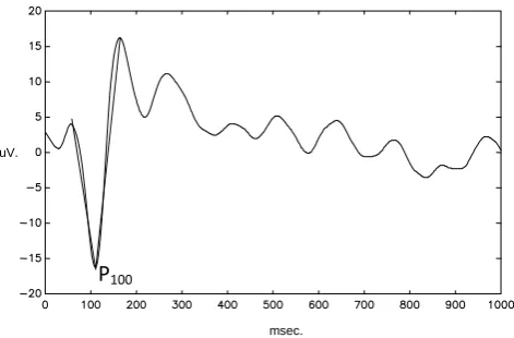
[image:2.595.63.276.90.272.2]P
100Figure 2. Visual evoked Potential.
originated it. In this case the stimuli are of visual type. A flash light generates a series of stimuli and the brain responses are acquired and averaged to get a waveform that in its first components frequently resembles a V letter. The points that demarcate this V are of specific diagnostic interest. The detection of a particular point (called P100 because often appears approximately 100ms after the stimulus), will be the problem to tackle. The detection must have into account the morphology of the signal (P100 context) and its time of occurrence because there are many other parts of the waveform with similar aspect [12]. Fig. 2 shows a Visual Evoked Potential example.
) ( ) ( )
(k n uk uk n
u − L L +
Backwark/Forward Time
) (k u
William-Zipser Neural Network
[image:3.595.349.509.81.207.2]Figure 3. Structure of the recurrent neural network model with shifted inputs. (PE problem).
Samples
Ou
tp
u
t
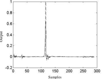
Figure 4. Neural network desire output and real output represent by discontinuous line and continuous line respectively (PE problem).
With these settings, the networks could converge to a good solution. Fig. 4 shows a close-up view of an evoked potential and the response of the network. The response peaks near exactly the P100 point. The size of the net was of only four neurons, the first of them being the output of the system and the initial state was set to zero both during training and testing.
A total of 44 evoked-potential sequences were used for training. A high number of detections (42) are within acceptable bounds (10 ms) of the correct point for the training sample. In the test sample, the results are slightly worse, but in this first test none of several generalization techniques available (early stopping, regularization term in error function…) or any special tuning were applied.
III. DYNAMIC ANALYSIS
A. 2-Pulse Problem
In the one-neuron dynamic equation two parameters appear feedback weight and bias. Considering the network training, the feedback weight is greater than one and the bias is next to zero. As a consequence, the network dynamics is based on two stable fixed points that
Samples
Ou
tp
u
[image:3.595.60.262.92.205.2]t
Figure 5. Neural Network Output without input and zero initial state (2-Pulse Problem).
Sa ddle Fixe d P oint Sta ble 2-C ycle
X1
X2
X3
X4
Figure 6. Fixed points and saddle unstable manifolds (PE problem).
are symmetric and an unstable fixed point situated in the origin. With respect to the phase trajectory, considering positive pulse, the state begins in the attraction domain of the positive stable fixed point and tends to this fixed point. In the case of the negative happens the opposite evolution: it tends towards the negative stable fixed point.
Fig. 5 shows the state going to one stable fixed point. In general, the initial state must stay inside the domain of attraction of the stable fixed point. In other hand, the evolution is slow. In fact, the state tends to another domain attraction with a minimal input change. In consequence, when it is present, the neural network input must be of a certain value in order to produce the transition to the adequate domain of attraction. In spite of this, it was obtained good results in generalization with varying pulse amplitudes.
B. Potential Evoked Problem
In this problem the dynamic is much more complex that in above case. In this problem appears a period two stable cycle and four saddle fixed points. In this case the unstable manifolds of the saddle fixed points (trayectories that diverge from saddle fixed points) are of dimension three and they are complex as can be appreciated in Fig. 6.
[image:3.595.83.266.241.378.2] [image:3.595.302.546.246.357.2]X1
X2
X3
X4
[image:4.595.302.537.84.227.2]k k
Figure 7. State evolution with external input. X1 represents the output of the
neural network. Iteration is codified by grey scale (PE problem).
Iter ations
Fe
ed
b
ac
k
we
ig
[image:4.595.54.315.86.185.2]h
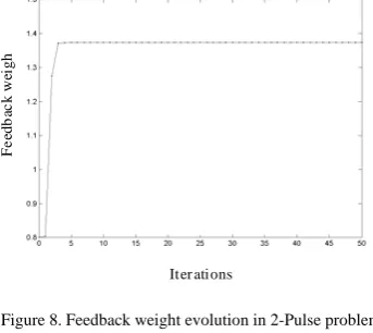
Figure 8. Feedback weight evolution in 2-Pulse problem.
Iterations
RM
S
E
[image:4.595.79.251.229.382.2]rror
Figure 9. Error evolution in the Evoked Visual Potential problem. The points correspond to the analyzed dynamics.
IV. ERRORVSDYNAMIC
The significative change in training with respect to the feedback weight is shown in fig. 8. In fact, the neuron changes dynamics from only stable fixed point to unstable, appearing two new stable fixed points, produced by saddle-node bifurcation [4].
Similarly, in the Evoked Potential problem exists a relationship between the network dynamics and error evolution. Fig. 8 shows that error abruptly decreasing. It is interesting to analyze the dynamics in the three error values
represented in X1
X2
X3
X4
Saddle Fixed Point Unstable Fixed Point Stable Fixed Point Saddle 2-Cycle
Stable 2-Cycle
[image:4.595.67.232.384.519.2]Figure 10. Greater value error point dynamic (PE problem).
Fig. 9.
Firstly, the greater error value dynamic is composed by three fixed points: stable, unstable and saddle, respectively, and three two-period orbits, two saddle and one stable (fig. 10). Actually, the most important aspect with respect to dynamics is that stable fixed point and the stable two-period orbits are situated in the saturation. It means that states tend to saturation without external inputs.
In the other hand, in the middle error point, the corresponding dynamics is composed by a saddle fixed point and a quasiperiodic-orbit. The error value is relatively high because quasiperiodic-orbit is near the saturation values, as show in fig. 11.
Finally, the dynamics corresponding to lower error values was that described in the previous section.
In the middle error dynamics appears a quasiperiodic orbit as a consequence of crossing a Neimark-Sacker bifurcation. In both problems, it is concluded that the error decreases by changing the dynamics and crossing a bifurcation of some kind.
X1
X2
X3
X4
Figure 11. Middle error point dynamic in PE problem. The saddle fixed point and quasiperiodic-orbit are represented by cross and points respectively.
V. INITIALIZATIONSTRATEGY
[image:4.595.310.547.497.609.2]neural network or the state derivative along time in the dynamic neural network. However, respect to the neural network dynamic this strategy is a bit restrictive because the origin is the only fixed point and is stable. In fact, the neural network is topologically equivalent to a linear stable system.
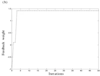
In order to design a new initialization strategy, consider the transitions produced by one-neuron network training in the 2-Pulse sample problem. In section 3 is shown that in the dynamic transition of a saddle-node bifurcation, the error decreases abruptly. It can be interesting to begin the training on other critical situations corresponding to other bifurcations (flip bifurcation). With respect to the feedback weight parameter this bifurcation appears when its value is (-1). Fig. 12 shows the relation between the error and feedback weight value. The feedback weight value tends to values greater than one, or the opposite way the optimal dynamic network is two stable fixed points. In other hand, it is hopeful because the dynamic network that appears in the flip bifurcation is one stable periodic double, in consequent the output network oscillate from positive value to negative. In order to classify the input pattern this dynamic behavior is not adequate.
The new strategy is based on starting in the bifurcation situations. Indeed, in the case of one-neuron network like the 2-pulse sample problem, it is compared experimentally a random classical initialization, with that beginning in the fold bifurcation, (feedback weight value one) and that starting in the flip bifurcation (feedback weight value -1).
In the fig. 13 is sketched the results of this comparison, the classical strategy, where the initial weight values come from a uniform distribution inside (-0.01, 0.01), fold and flip bifurcation initializations. It is shown that the best strategy corresponds to fold bifurcation initialization. The second is the flip bifurcation initialization that still improves the classical initialization. Inside each 3-dimensional histograms appear many weights with similar error values. These are caused by the local minima in the error surfaces towards which the weights converge.
Ite rat ion s
RM
S
E
rror
(a)
I ter at ions
F
ee
d
ba
ck
w
ei
g
ht
[image:5.595.341.505.87.211.2]( b)
Figure 12. 2-Pulse problem training process beginning with feedback weight (-1). (a) Error evolution and (b) feedback weight evolution.
(a) (b)
(c)
Iterations Iterations
Iterations
RMS Error RMS Error
RMS Error
C
o
unt
N
o
rm
al
iz
ed
Co
u
n
t
N
o
rm
al
iz
ed
Co
u
nt
No
rm
a
li
[image:5.595.319.531.274.427.2]zed
Figure 13. Error normalized distribution in the 2-pulse problem. (a) classical strategy, (b) fold bifurcation initialization, and (c) flip bifurcation initialization.
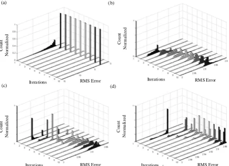
In the Potential Evoked problem is necessary to redefine the new strategy to a multidimensional dynamic neural network system. In fact, here appears a new type of bifurcation, the Neimark-Sacker. The bifurcation conditions generalized to multidimensional systems are: an eigenvalue equal to 1 to reflect saddle-node bifurcation, an eigenvalue equal to (-1), in the case of a flip bifurcation, and two conjugate complex eigenvalues in the unit circle in the Neimark-Sacker bifurcation.
In order to implement this new strategy generalization, the initial weight matrix must be particularised. The algorithm of matrix initialization consists firstly in generating n random weights from a uniform distribution, where n corresponds to the number of neurons. Next, the first value is assigned to 1, in case to begin on saddle-node bifurcation or (-1) in flip bifurcation. The third step consists in a permutation of this number and the inclusion of this vector as the diagonal in a diagonal matrix D. In the last step it is generated a n x n random rotation matrix T, so the definitive initial weight matrix is
T
D
T
W
Output=
−1In order to guarantee that the neural network begins in the bifurcation it is necessary also that the bias and input weights are zero. The Neimark-Sacker bifurcation initialization is similar that above case, except that the matrix D include a rotational matrix characterized by two conjugate complex eigenvalues in the unit circle:
( )
( )
( )
( )
⎥ ⎥ ⎥ ⎥ ⎥ ⎥ ⎥ ⎥ ⎦ ⎤ ⎢ ⎢ ⎢ ⎢ ⎢ ⎢ ⎢ ⎢ ⎣ ⎡ − = n v sen sen v D 0 0 cos cos 0 0 0 1 L L L M O M M M M M M O L L L θ θ θθ (3)
where θ is random value.
Fig. 14 is obtained in a similar way as fig. 13. This figure shows that the multidimensional bifurcation strategy results are much better than that of the classical strategy.
VI. CONCLUSION
An algorithm for determining the initial recurrent network based on bifurcation theory was successfully developed. This new strategy was applied to two problems. The first problem is very simple, to allow easier visualization of the relation between dynamics and error and it was easy to explain the good results of the bifurcation strategy in this problem. The potential evoked problem was much more complex to train but it obtained similar results and it showed the benefits of inducing initial situations of bifurcation in training process. In future works this result can be generalized to other problems and add in the training process some information constraints in the dynamics.
REFERENCES
[1] R. Hush and Bill G. Horne, “Progress in supervised Neural Networks”,
IEEE Signal Processing Magazine. January 1993.
[2] C. Robinson, Dynamical Systems. Stability, Symbolic Dynamics, and Chaos. Ed. Inc. Press CRC, 1995.
[3] J. Hale, H. Koςak, Dynamics and Bifurcations, New York: Springer-Verlag, 1991.
[4] Y. A. Kuznetsov, Elements of Applied Bifurcation Theory, New York : Springer-Verlag, Third Edition, 2004.
[5] C. M. Marcus and R. M. Westervelt, “Dynamics of Iterated-Map Neural Networks”, Physical Review A, vo. 40, 1989, pp: 501-504 .
[6] Jine Cao, “On stability of delayed cellular neural networks”, Physics Letters A, vol. 261(5-6), 1999, pp: 303-308.
[7] Tino et al. Attractive Periodic Sets in Discrete-Time Recurrent Networks (with Emphasis on Fixed-Point Stability and Bifurcations in Two-Neuron Networks)”. Neural Computation , vol. 13(6), 2001, pp: 1379-1414. [8] F. Pasemann. “Complex Dynamics and the structure of small neural
networks”, In Network: Computation in neural system, vol. 13(2), 2002, pp: 195-216.
[9] F. Pasemann. “Synchronous and Asynchronous Chaos in Coupled Neuromodules”. International Journal of Bifurcation and Chaos, vol. 9(10), 1999, pp: 1957-1968.
[10] X. Wang, Discrete-Time Dynamics of Coupled Quasi-Periodic and Chaotic Neural Network Oscillators, International Joint Conference on Neural Networks, 1992.
[11] R. L. Marichal, J. D. Piñeiro, L. Moreno, E. J. González, J. Sigut. “Bifurcation Analysis on Hopfield Discrete Neural Networks”, WSEAS Transaction on System, Vol 5, 2006, pp:119-125.
[12] D. Regan. Human Brain Electrophysiology. Evoked Potentials and Evoked Magnetic Fields in Science and Medicine. Elsevier, 1989. [13] R.Fletcher. Practical Methods of Optimization, John Wiley & Sons
Second Edition, 2000.
[14] Y. Bengio, P. Simard, P. Frasconi. “Learning Long-Term Dependences with Gradient Descent is Difficult”. IEEE Transaction on Neural Networks, Vol. 5, 1994,pp:157-166.
[15] J. D. Piñeiro, R. L. Marichal., L. Moreno, J. Sigut, I. Estévez, R. Aguilar., J. L. Sánchez., J. Merino. “Evoked Potential Feature Detection with Recurrent Dynamic Neural Networks”. International ICSC/IFAC Symposium on Neural Computation, September 1998, Viena.
[16] G. Thimm, E. Fiesler. “High-order and multilayer perceptron initialization ”, IEEE Transactions on Neural Networks, vol. 8 (2), 1997, pp: 349-359.
(a) (b)
(c) Itera tions (d)
Co u n t N o rm al ized RMS Error Iterations Iterations Iterations
RMS Error RM S Error
[image:6.595.311.548.252.423.2]RMS Error C oun t No rm al ized Co u n t No rm a li z ed Co u n t No rm al ized