Abstract—Applying nonequilibrium statistical mechanics we focus on nonequilibrium corrections Δs to entropy and energy of the fluid in terms of the nonequilibrium density distribution function, f. We also evaluate coefficients of wave model of heat such as: relaxation time, propagation speed and thermal inertia. With these data a quadratic Lagrangian and a variational principle of Hamilton’s type follows for a fluid with heat flux in the field representation of fluid motion. We discuss canonical conservation laws and show the satisfaction of the second law under the constraint of these conservation laws.
Index Terms— conservation laws, Grad solution, variational principles, wave equations.
I. INTRODUCTION
We use the framework of extended thermodynamics of fluids to discuss variational principles for irreversible energy transfer and help that can be obtained from statistical theories when describing nonequilibrium thermodynamic systems and evaluating kinetic or flux-dependent terms in energies and macroscopic Lagrangians. Especially, we treat statistical aspects of thermodynamic and transport properties of nonequilibrium fluids with heat flow by applying an analysis that uses Grad’s results [1] to determine nonequilibrium corrections Δs or Δe to the energy e or entropy s in terms of the nonequilibrium density distribution function f. To find corrections to the energy e or kinetic potential L we use corrections Δs and a relationship that links energy and entropy representations of thermodynamics. We also evaluate coefficients of wave model of heat, such as: relaxation time, propagation speed and thermal inertia factors, g and θ. With these data we formulate a variational principle of Hamilton’s or least action type for fluids with heat flux in the field or Eulerian representation of fluid motion. Analyzing the variational extremum we display an approach that adjoints a given set of constraints to a kinetic potential L and transfers the original variational formulation to the space of associated Lagrange multipliers. By considering limiting reversible process we evaluate canonical components of energy-momentum tensor
Manuscript received March 24, 2007. This work was supported by the Statute Grant Simulation and Optimization of Thermal and Mechanical Separation of Substances and Energy Conversion. S. Sieniutycz is with the Faculty of Chemical and Process Engineering at Warsaw TU, 1 Waryńskiego Street, Warszawa, 00645 Poland (phone: 00-48228256340; fax: 00-48228251440; e-mail: sieniutycz@ ichip.pw.edu.pl).
along with associated conservation laws. We show that despite of the generally non-canonical form of conservation laws produced by Noether’s theorem the approach that adjoints constraints to given kinetic potential works efficiently. In fact, the approach leads to exact imbedding of constraints in the potential space of Lagrange multipliers, implying that the appropriateness of the constraining set should be verified by physical rather than mathematical criteria. Our analysis shows that the approach is particularly useful in the field (Eulerian) description of transport phenomena, where equations of thermal field follow from variational principles containing state adjoints rather than original physical variables. Exemplifying process is hyperbolic heat transfer, but the approach can also be applied to coupled parabolic transfer of heat, mass and electric charge. With various gradient or non-gradient representations of physical fields in terms of state adjoints (quantities similar to those used by Clebsch in his representation of hydrodynamic velocity) useful action-type criteria emerge. Symmetry principles are effective, and components of the formal energy-momentum tensor can be found. The limiting reversible process, with ignored random effects, provides a suitable reference frame. Focusing on heat flow, our work represents, in fact, an approach that shows the methodological advantage of approaches borrowed from the optimal control theory in variational descriptions of irreversible transport phenomena.
II. HELP FROM STATISTICAL THEORIES AND OPTIMIZATION-TYPE APPROACH
Statistical theories are useful [1] to evaluate nonequilibrium corrections to energy and other thermodynamic potentials in situations when a continuum is inhomogeneous and this inhomogeneity is associated with presence of irreversible fluxes. To illustrate benefits resulting from suitable findings in the field of nonequilibrium statistical thermodynamics, heat transfer in locally non-equilibrium fluids is analyzed [2].
Quite essential in these analyses is the connection between various representations of thermodynamics of nonequilibrium fluids and a relationship (resembling the Gouy-Stodola law) that links energy and entropy pictures. Thanks to this relationship nonequilibrium corrections to the energy can be found from those known for the entropy of the Grad’s theory. These energy corrections will next be used to construct suitable kinetic potentials L and formulate variational principles
In this paper we work in the energy and Lagrangian
Statistical Aspects in Variational Principles with
Heat Flow
representations of thermodynamics and focus on formulation of a linear variational description for heat transfer in incompressible continua. While the linearity of the theory is certainly an approximation, it is simple and lucid enough to illustrate a (relatively unknown) variational approach based on adjoining known process equations as “constrains” to a “kinetic potential L” (the integrand L of an action functional).
The present approach is optimization-type; it differs from more conventional variational ones in that the action functional is systematically constructed rather than assumed from the beginning. Once a variational theory is developed for an assumed L it may easily be modified for improved kinetic potentials which take more subtle effects into consideration. Equations of constraints (reversible or irreversible) follow in the form of their “representations” in the space of Lagrange multipliers; they are extremum conditions for the action containing a composite (constraint involving) Lagrangian Λ or its gauge counterparts. As long as representations describing physical variables of state in terms of Lagrange multipliers are known in their explicit form, the whole variational formalism can be transferred to the adjoint space of these multipliers, i.e. a variational principle can be formulated in this (adjoint) space. The Lagrangian can also be used to obtain the matter tensor for the continuum with heat flow, and associated conservation laws.
Finally we show that the acceptance of canonical conservation laws, constructed for a limiting reversible process, along with variational extremum conditions assures the satisfaction of the second law of thermodynamics, the property that renders the variational theory considered a candidate to be the physical one. Moreover, formal conservation laws, evaluated from Noether’s theorem, are the process integrals that may provide additional insight on the transformation of energy in the irreversible system.
III. ENERGY AND ENTROPY REPRESENTATIONS IN THERMODYNAMICS OF HEAT FLOW
Now our task is to recall some basic knowledge on the thermodynamics of heat flow without local equilibrium. A process description will be developed that will next be used to construct suitable lagrangians, variational principles and conservation laws. We work in the framework of extended thermodynamics of fluids [3]. We restrict ourselves to incompressible, one-component continuum with heat flow.
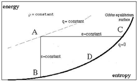
Consider a continuum with the heat flow at a nonequilibrium state, say A, off but near the Gibbs surface, when the local equilibrium assumption is inapplicable, Fig. 1. The energy at the state A is the nonequilibrium internal energy. This internal energy depends not only on the usual state variables (wherever they have meaning), but also on nonequilibrium variables such as heat flux or diffusive entropy flux. Here we select the heat flux, q, as the nonequilibrium variable of choice. It is treated as an unconstrained internal variable which relaxes to equilibrium. Nonequilibrium energy density of a continuum, ρe, or its specific energy e, is a function of density ρ, specific entropy s
and diffusive entropy flux js or heat flux q. For a continuum as a stable macroscopic system, its equilibrium internal energy density ρeeq is the minimum of ρe with respect to unconstrained js or q, at constant ρ and s. As ρ = v-1, the reciprocal of specific volume, the minimum of ρe (or e itself) with respect to js or q occurs at constant entropy s and volume v which are proper variables at which the energy attains minimum at equilibrium. This is in agreement with basic thermodynamics [4]. Since js or q are a diffusive fluxes, the minimum occurs for js = 0 or q=0. For a given nonequilibrium state at a point A in Fig.1, two equilibrium reference states, at points B and C, say, correspond, respectively, to the energy and entropy representation. A researcher knowing entropy s (e. g., from distribution function f
[image:2.612.328.550.352.483.2]corresponding to A) formulates his description of state A in terms of equilibrium parameters at B, for a set of variables, here the entropy flux js. Yet, one who knows energy e can base his view on the heat flux q and equilibrium at C. When point A moves the equilibrium states (B and C) vary. The conventional picture of motion in terms of Hamilton's principle corresponds to following the behavior of B and the kinetic energy of entropy flux, whereas the kinetic theory view corresponds to tracking of C and the deviation of entropy from equilibrium. The transition from one view to the other is possible [2].
Fig. 1. Diverse reference equilibria (B, D, C, etc.) for a given state A.
It is important to realize that for a single nonequilibrium state the use of the entropy representation and energy representation establish two different equilibrium states located on the Gibbs surface. This of course, is because of the difference in what is held constant. The distance between two discussed equilibrium states (B and C) increases with the distance of the state A from the Gibbs surface. This distance can also be measured in terms of the modulus of the flux js or in terms of the differences Δe = AB or Δs = AC. When the curvature of the Gibb's surface can be neglected, corresponding to the near-equilibrium situation, the two disequilibrium excesses are linked by an equality resembling the Gouy-Stodola law
the heat flux q or the entropy flux, js.
IV. NONEQUILIBRIUM CORRECTIONS TO ENERGY OR ENTROPY IN TERMS OF DISTRIBUTION FUNCTION F
It is essential that the entropy representation is assumed in the Grad’s formalism of the kinetic theory [1]. Hence the specific energy of an ideal gas or fluid with heat at the point A is equal to the specific energy at equilibrium C in Fig. 1. The reference temperatures and pressures that appear in the expressions of kinetic theory are T(C) and P(C). From the formalism one finds disequilibrium corrections Δs or Δe in terms of the non-equilibrium density distribution function f. Here we recapitulate the results of several different works [3]-[6] all using Grad’s [1] solution of the Boltzmann equation in macroscopic predictions for dilute gas of rigid spheres.
The molecular velocity distribution function, f, out of equilibrium but close to it is given as
) 1 )( ( )
(C = feq C +ϕ1
f (2)
where feq is the local equilibrium (Maxwell-Boltzmann) distribution pertaining to the entropy representation equilibrium (point C, Fig. 1). f and feq are scalars, but functions of the peculiar velocity C = c - u, and ϕ1 is a function of the deviation from equilibrium. This deviation is expressed in terms of the gradT in the Chapman-Enskog method and in terms of the heat flux q in the Grad's method. Using Eq. (2) in the entropy definition, one integrates the expression flnf over all of the space of the molecular velocity c,
ρs =−kB
∫
flnfdc (3) Proceeding with development of ρs up to second order in φ1, one obtains (1) (2),s s eq s
s ρ ρ ρ
ρ = + + with local equilibrium entropy ρ =−k
∫
feq feqdcB eq
s ln (4)
and nonequilibrium correction
0 ln
1 )
1
( =− =
∫
f f dck
ρs B eqϕ eq . (5)
Again, this proves that one deals with the entropy representation where the entropy is maximum at equilibrium. A counterpart of the above equation in the energy representation
2 0,
1 )
1
( =−
∫
f mc dc=ρ eq
e ϕ (6)
would correspond to the minimum energy. The second order correction to the entropy density (in entropy representation) is
∫
− = Δ=ρ s k f dc
ρs(2) B eq 12
2
1 ϕ
(7) Hence, in view of the relation between Δe and Δs implied by Fig. 1 or Eq. (1)
∫
−− =
Δe k Tρ feq dc
B 1 12
2
1 ϕ (8)
Since the state A is close to the equilibrium surface, the multiplicative factors containing conventional thermodynamic variables can always be evaluated at arbitrary equilibrium points (B or C in Fig. 1). However, in Eqs. (1), (9) and (10), they were evaluated (in the kinetic theory) for the case of the isoenergetic equilibrium (point C, Fig. 1). The function ϕ1,
obtained in Grad's method when the system's disequilibrium is maintained by a heat flux q is
C )C.q
2 5 2
1 )( /
( 5
2 2 2 2
1= m PkBT m − kBT
φ (9)
where m is the mass of a molecule ([1], [3]). From Eqs. (7), (8) and (9) one obtains for the entropy deviation
( / 2) 2
5
1 m ρPk T q
s=− B
Δ (10)
and for the energy deviation, Eq. (1), with entropy flux js = qT-1
2 2 2 2 2
2 1 ) / ( 5 1
s s
Bρ ρ g
k m
e= j = − j
Δ (11)
Equations (10) and (11) hold to the accuracy of the thirteenth moment of the velocity [1]. When passing from Eq. (10) to (11) state equation P = ρkBTm-1 is used and a constant g is defined as
. 5 2 5
2
2 2
B
B k
m Pk mT
g ≡ ρ = (12) Here we abandoned the entropy representation. Pressure in Eqs. (9) and (12) is that of an ideal gas, given by the definition used in the kinetic theory (Grad 1958 [1]). Eq. (11) with constant g defined by Eq. (12) is the characteristic feature of the ideal monoatomic gas (dilute Boltzmann gas composed of hard spheres). For arbitrary fluids (polyatomic gases, dense monoatomic gases and liquids) one can retain the form of the last expression in Eq. (11) by using a general definition of g
obtained by noting that
g(ρ,s)≡ρeq2(∂2e/∂js2)eq (13) In the ideal gas case the derivative ∂2e/ 2
s
j
∂ = (2/5)(m2/kB2ρ2) from Eq. (11) and the definition (12) is recovered form definition (13). Equation (13) is consistent with a hypothesis about the equality of the kinetic and static nonequilibrium energy corrections in a thermal shock-wave front [5]. The hypothesis can be used to compute (∂2e/∂j
s2)eq for arbitrary fluids as T/(ρcpG) and hence g as Tρ/(cpG), where G is the shear modulus. Equilibrium values of thermodynamic parameters can be applied in such expressions. For an ideal gas the shear modulus is just the pressure P (the result of Maxwell) and cp = 5kB/(2m). These results allow one to recover definition (12) from the expression g = Tρ/(cpG); they support the hypothesis mentioned above. Yet, for the purpose of general considerations the use of the implicit dependence of g on the basic variables (ρ, s) is often enough, i. e., the function g(ρ, s) will be used when passing to arbitrary fluids. Use of some entropy flux adjoints, as and is, is suitable. They are defined, respectively, by equations
as(s,ρ,js)=∂Δe(s,ρ,js)ρ,s/∂js =gρ−2js (14)
and
i ( , ,j )= −1j = v = (u −u) s s
s s
s s ρ gρ gs gs (15)
The entropy diffusion velocity vs = us - u = js/ρs = js/ρs appears in Eq. (15). One may also introduce therein the product kBgs which has the dimension of mass. For the ideal gas this product is ms = 2/5(m2sk
is equal to the equilibrium temperature T(ρ, s) which is both the measure of mean kinetic energy of an equilibrium and the derivative of energy with respect to the entropy. This equality emerges because, above, we have chosen the entropy flux js, not the heat flux q, as the nonequilibrium variable in energy function e. If one differentiates the nonequilibrium entropy s
with respect to the energy holding q constant, then a quantity
T(C) of Jou at al ([3]) follows, which differs from the reciprocal of the corresponding equilibrium temperature Teq by a term quadratic in q. In general, the "nonequilibrium temperatures" (understood as the fifth moment of the nonequilibrium density functions) are not the measures of mean kinetic energy.
The knowledge of inertial coefficients, such as g, from statistical mechanics considerations helps calculate two basic quantities in the model of heat transfer with finite wave speed. They are: thermal relaxation time τ and and the propagation speed, c0. Of several formulae available that link quantities τ and g, probably the following expression
τ = g(ρT)−1
k (16)
is most useful ([6], p. 199). It links thermal relaxation time τ with thermal conductivity k, inertia g and state parameters of the system. As, by definition, the propagation speed of the thermal wave c0= (a/τ)1/2, where a= k /(ρcp) is thermal diffusivity, the quantity c0 may be determined from the formula
. g )
(
2 / 1 2
/ 1
0 ⎟⎟
⎠ ⎞ ⎜ ⎜ ⎝ ⎛ = =
p
c T a
c
τ (17)
Substituting to this expression the ideal gas data, i.e. g of Eq. (12) and cp = 5kB/(2m), yields propagation speed in the ideal gas
2 / 1 2
/ 1
0 g ⎟
⎠ ⎞ ⎜ ⎝ ⎛ = ⎟ ⎟ ⎠ ⎞ ⎜ ⎜ ⎝ ⎛ =
m T k c
T
c B
p
(18) (thermal speed). Thus the results of nonequilibrium statistical mechanics help to estimate numerical values of damped-wave model of heat transfer. The coefficients τ and c0 are used below in a variational principle for wave heat transfer. One more coefficient that is quite useful in the wave theory of heat is that describing a thermal mass per unit of entropy
θ=Tc0−2, (19)
[6]. For the ideal gas, Eq. (18) yields the coefficient θ as θ=mkB−1 (20) We can now set a variational description for linear wave heat flow satisfying Cattaneo model.
V. TESTING APPROACHES ADJOINING A GIVEN SET OF CONSTRAINTS TO A KINETIC POTENTIAL
For the heat conduction process described in the entropy representation by the Cattaneo equation of heat and the conservation law for internal energy, the set of constraints is
2 0
0 2 0
= ∇ + + ∂ ∂
e
c t
c τ ρ
q q
(21)
and
0 . = ∇ + ∂ ∂
q t
e
ρ
, (22) where the density of the thermal energy ρe satisfies dρe = ρcvdT,
c0 is propagation speed for the thermal wave, τ is thermal
relaxation time, and D=c02τ is the thermal diffusivity. Equation (22) assumes conservation of the thermal energy (rigid medium and neglect of the viscous dissipation). In irreversible processes the paths of entropy or energy differ from those of the matter. For simplicity we assume constant values of involved fields at the boundary. We ignore the vorticity properties of the heat flux.
The energy-representation of the Cattaneo equation, 2 + 2 +∇ =0
∂ ∂
T c t
c s
s
s s
τ j j
(23) uses diffusive entropy flux js instead of heat flux q. The coefficient cs is defined as
2 / 1 1)
( −
≡ ρ vθ
s c
c , (24)
where θ=T 2 0−
c , and thermal diffusivity ρ 2τ
0
c cv
≡
k . Equation
(23) is Kaliski’s equation [6]. For an incompressible medium one may apply this equation in the form
0
2 0 2 0
= ∇ + + ∂ ∂
s s s
c t
c τ ρ
j
j (25)
which uses the entropy density ρs as a field variable.
Yet, in this paper we focus on action and extremum conditions in entropy representation (Eqs. (21) and (22) in variables q and ρe). For Eqs. (23) - (25) another action approach will be developed in a complementary paper. Action approaches should be distinguished from entropy-production approaches [6], [7]. Here an action is assumed that absorbs constraints (21) and (22) by Lagrange multipliers, the vector ψ and the scalar φ
. )} . ( ) .(
2 1 2 1 2 1
{ 2
0 2 0 2 2 2 0 2
, 1
2
1
dVdt t
φ
c t c c
A e e e
t
V t
q q
q
ψ
q
∇ + ∂ ∂ + ∇ + + ∂ ∂ + − −
=
∫
− ρ ρτ ε
ρ
ε . (26)
As kinetic potentials can be very diverse, the conservation laws for energy and momentum substantiate the form (26). In Eq. (26), ε is the energy density at an equilibrium reference state, the constant which ensures the action dimension for A, but otherwise is unimportant. Yet we assume that the actual energy density ρe is close to ε, so that the variable ρe can be identified with the constant ε in suitable approximations.
We call the multiplier-free term of the integrand of Eq. (26)
} {
2
1 2 2
2 0 2
1 ρ ε
ε − −
≡ −
e c
L q (27)
of heat”, and the nonequilibrium internal energy, ρe. To secure correct conservation laws, no better form of L associated with a non-linear model was found in the entropy representation. The theory obtained in the present case is a linear one.
Vanishing variations of action A with respect to multipliers ψ and φ recover constraints, whereas those with respect to state variables q and ρe yield representations of state variables in terms of ψ and φ. For the accepted Hamilton-like structure of L,
c φ
τ
t − + ∇
∂ ∂ = 2 0 ψ ψ
q (28)
and . t e ∂ ∂ − −∇ = φ
ρ ψ (29) These equations enable one to transfer variational formulation to the space of Lagrange multipliers.
For the accepted structure of L, the action A, Eq. (26), in terms of the adjoints ψ and φ is
)
. 2 1 . 2 1 21 2 2 2 2
0 2 0 1 2 , 1 dVdt t c t c A t
tV ⎪⎭
⎪ ⎬ ⎫ − ⎟ ⎠ ⎞ ⎜ ⎝ ⎛ ∂ ∂ + ∇ − ∇ + ⎪⎩ ⎪ ⎨ ⎧ ⎜ ⎝ ⎛ − ∂ ∂
=
∫
− φ φ ετ
ε ψ ψ ψ (30)
Its Euler-Lagrange equations with respect to ψ and φ are
0 . 1 1 2 0 2 0 2 0 2 0 = ⎟ ⎠ ⎞ ⎜ ⎝ ⎛ ∂ ∂ + ∇ ∇ − ⎟ ⎠ ⎞ ⎜ ⎝ ⎛ − + ∇ ∂ ∂ + ⎪⎭ ⎪ ⎬ ⎫ ⎪⎩ ⎪ ⎨ ⎧ ⎟ ⎠ ⎞ ⎜ ⎝ ⎛ − + ∇ ∂ ∂ ∂ ∂ t c t c c t c t φ φ τ τ φ τ ψ ψ ψ ψ
ψ (31)
and
. 0 .
. 02 ⎟=
⎠ ⎞ ⎜ ⎝ ⎛ − + ∇ ∂ ∂ ∇ + ⎟ ⎠ ⎞ ⎜ ⎝ ⎛ ∂ ∂ + ∇ ∂ ∂ − φ τ φ c t t t ψ ψ
ψ (32)
It is easy to see that (31) and (32) are the original equations of the thermal field, eqs. (21) and (22), in terms of the potentials ψ and φ. Their equivalent form below shows damped wave nature of the transfer process. In fact, Lagrange multipliers ψ and φ of this (sourceless) problem satisfy certain inhomogeneous wave equations. In terms of the modified quantities Ψ and Φ satisfying Ψ = ψ 2
0
τc and Φ = - φτ 2 0
c
these equations are
2 . 0 2 2 0 2
2Ψ Ψ Ψ =q
∂ ∂ + ∂ ∂ − ∇ t c t
c τ (33)
and . 2 0 2 2 0 2 2 e t c Φ t c Φ Φ ρ
τ ∂ = ∂ + ∂ ∂ −
∇ (34)
As both state variables (q, ρe) and adjoints (ψ, φ) appear in these equations, they represent mixed formulations of the theory. They show that for given q and ρe thermal transfer can be broken down to potentials. The situation is similar to that in electromagnetic theory or in gravitation theory, where the specification of sources defines the field potentials. An important case is the reversible “ballistic” process with τ→∞ when undamped thermal waves propagate with the speed c0 and satisfy d' Alembert's equation for potentials and energy density.
VI. SOURCE TERMS IN INTERNAL ENERGY EQUATION The method of direct substitution of representations into L is
valid only for linear constraints that do not contain sources. This may be exemplified when the internal energy balance contains a source term a’q2, where a’ is a positive constant. The augmented action integral (26) should now contain the negative term - a’q2 in its φ term. The energy density representation remains unchanged, whereas the heat flux representation follows in a generalized form
) (
) 2 1
( a c02 1 ∂t − τ +c02∇φ
∂ ′
−
= − ψ ψ
q φ (35)
Substituting Eqs. (29) and (35) into action A of Eq. (26) (L of Eq. (27)) shows that the action based on the accepted kinetic potential L in terms of the potentials acquires the form
)
dVdt c t c a c A ttV ⎭
⎬ ⎫ ∇ + ⎪⎩ ⎪ ⎨ ⎧ ⎜ ⎝ ⎛ − ∂ ∂ ′ − = − −
∫
2 20 2 2 0 2 0
1 (1 2 )
2 1 2 , 1 φ τ φ
ε ψ ψ
dVdt t
t
tV ⎪⎭
⎪ ⎬ ⎫ ⎪⎩ ⎪ ⎨ ⎧ + ⎟ ⎠ ⎞ ⎜ ⎝ ⎛ ∂ ∂ + ∇
−
∫
−1 2 22 1 . 2 1 2 , 1 ε φ
ε ψ . (36)
However the Euler-Lagrange equations for this action are not process constraints in terms of potentials. The way to improve the situation is to substitute the representations to a transformed augmented action in which the only terms rejected are those that constitute total time or space derivatives. When this is applied and total derivatives are rejected, a correct action follows
)
dVdt c t c a c A ttV ⎭
⎬ ⎫ ∇ + ⎪⎩ ⎪ ⎨ ⎧ ⎜ ⎝ ⎛ − ∂ ∂ ′ − = − −
∫
2 20 1 2 0 2 0
1 (1 2 )
2 1 2 , 1 φ τ φ
ε ψ ψ
dVdt t
t
tV ⎪⎭
⎪ ⎬ ⎫ ⎪⎩ ⎪ ⎨ ⎧ + ⎟ ⎠ ⎞ ⎜ ⎝ ⎛ ∂ ∂ + ∇
−
∫
−1 2 22 1 . 2 1 2 , 1 ε φ
ε ψ (37)
Action (37) yields the proper Cattaneo constraint (21) and the generalized balance of internal energy which extends equation (22) by the positive source term a’q2. Yet, due to the presence of the source, the formulation does not exist in the original four-dimensional original space (q, ρe), and, if somebody insists to exploit this space plus a necessary part of the potential space, the following A is found from Eqs. (21), (29), (35) and (37)
dVdt c c a A e t V t } 2 1 2 1 2 ) ' 2 1
{( 2 2 2
0 2 2 0 , 1 2 1 ε ρ φ
ε − − +
=
∫
− q (38)VII. CANONICAL MATTER TENSOR AND CONSERVATION LAWS Here we determine conservation laws for the energy and momentum for Noether’s theorem for our model at its reversible limit. The energy-momentum tensor is defined as
(
)
− Λ⎥ ⎥ ⎦ ⎤ ⎢ ⎢ ⎣ ⎡ ∂ ∂ ∂ Λ ∂ ∂ ∂
≡
∑
jkl j l k
l jk v v G δ χ
χ (39)
the differentiation by parts. In our problem } 2 1 ) ( 2 1 ) ( 2 1
{ 2 0 2 2
1 ε
ε − ∇ −
∂ ∂ =
Λ − c φ
t
φ (40)
In terms of the physical variables
} 2 1 2 1 2 1
{ 2 2
0 2 2
1 ρ ε
ε − −
=
Λ −
c q
e (41)
The matter tensor G = Gjk has the following structure
⎥ ⎦ ⎤ ⎢ ⎣ ⎡ − = E Q Γ T
G , (42)
where T is the stress tensor, Γ is the momentum density, Q is the energy flux density, and E is the total energy density.
When external fields are present, the balance equations are satisfied rather than conservation laws
0 = ∂ Λ ∂ + ⎟ ⎟ ⎠ ⎞ ⎜ ⎜ ⎝ ⎛ ∂ ∂
∑
j k k jk G χχ (43)
for j, k = 1, 2..4. Equation (43) is the formulation of balance equations for momentum (j = 1, 2, 3) and energy (j = 4).
The momentum density for the mass flow of the medium at rest is, of course, J=0, where J is the mass flux density. The momentum component of heat flow in the frame of J=0 can be determined from Lagrangian (40) and Eq. (39) for j=4
(
)
aa φ t φ t φ x φ G
G 4 1 (∇ )
∂ ∂ − = ∂ ∂ ∂ Λ ∂ ∂ ∂ − = −
= ε−
α
α (44)
Using “reversible” representations =c2∇φ
0
q and
ρe=-∂ϕ/∂t leads to the momentum density of heat in physical variables α α α α ε ρ q c q c
G e 2
0 2
0
4= − ≅ −
− =
Γ (45)
Clearly, Γ vanishes in the Fourier’s case (c0→∞). The stress tensor Tab has the form
Tab=−ε−c2(∇φ)a(∇φ)b−δabΛ
0
1 (46)
or in physical variables
Tαβ =−ε−c−2qαqβ−δαβΛ
0
1 (47)
After substituting stationary Lagrangian into Tab we obtain
} 2 1 2 1 2 1
{ 2 2 02 2
1 2
0
1 α β δαβε ρ ε
αβ=−ε−c−q q − − − c− −
T e q (48)
This quantity represents stresses caused by the pure heat flow; it vanishes at equilibrium.
Canonical energy density follows as the Legendre transform of the Lagrangian Λ with respect to rate change of φ in time
} 2 1 ) ( 2 1 ) ( 2 1
{ 2 2
0 2
1 ε
ε + ∇ +
∂ ∂
= − c φ
t φ
E (49)
or in terms of the physical variables
e e c q c q G E ρ ε ε ρ
ε + + ≅ +
= = − 2 0 2 2 2 2 0 2 1 44 2 1 } 2 1 2 1 2 1
{ (50)
The energy of resting mediun with heat flux is the sum of the kinetic energy of heat and equilibrium thermal energy.
Finally, we find density of energy flux in both frames
(
)
ββ ρ 2( )
0 1
4 ε c φ
x φ t φ
G β = e ∇
∂ ∂ ∂ Λ ∂ ∂ ∂
≡ − (51)
β β β
β Q ε ρ q q
G4 = = −1 e ≅ . (52)
The associated conservation laws for the energy and momentum have the form
(
q)
q e t e
c ρ ε ρ
ε 2 2 1
0
1 )/ .
2 1
( − − + ∂ =−∇ −
∂ (53)
(
)
{
( 2)}
2 1 2 2 1 2 0 2 2 1 2 0 1 1 2
0 ) .
( ε ρ δ ε ρ
ε α =∇ − α β+ αβ − +
∂
∂ − − − − −
e
e c q q c
t q c
q . (54)
VIII. ENTROPY PRODUCTION AND SECOND LAW OF THERMODYNAMICS
In the variational theory of heat the satisfaction of the second law is not explicit, thus we shall derive it by considering entropy properties. The internal and total energy satisfy the equality
12ε−1c0−2q2+ρe(ρs)=E (55) It shows that entropy density ρs is a function Sv of E and q, hence ) 2 1 ( )
( e =Sv E− −1c0−2q2
s ρ ε
ρ . (56)
Thus at the constant mass density the differential of Sv satisfies an extended Gibbs equation
q q.
q T dE T c d
c E d
dSv s e 2
0 1 1 1 2 2 0 1 ) 2 1 ( ) (∂ ∂ − − − = − − − − −
= ρ ρ ε ε (57)
Taking into account that c0 = (a/τ)1/2 = (k/(ρcvτ))1/2, where k
is the thermal conductivity, one findsc0−2=ρcvτ/k = εT-1τk−1,
and the above differential expressed in terms of k is q q.d T
dE T
dSv= −1 − −2τk−1 (58)
Calculating the four-divergence of the entropy flow (∇,∂/∂t) and using the global conservation law for the energy
E we obtain in terms of expressions containing k or c0
⎟ ⎠ ⎞ ⎜ ⎝ ⎛ ∂ ∂ − ∇ − = ⎟ ⎟ ⎠ ⎞ ⎜ ⎜ ⎝ ⎛ ∂ ∂ − ∇ = ∇ + ∂ ∂ − t T k kT t Tc T T t
Sv q q q q τ q
ε .
1 .
)
.( 2 2
0
1 (59)
But, since Eq. (21) is a simple transformation of the Cattaneo equation we arrive at the expression
2 2 2 2 0 2 ) .( s v a kT T c T t S j q q
q = ≡ =
∇ + ∂ ∂
ετ , (60)
where a = k-1 is the thermal resistance. This equation describes the second law of thermodynamics in the identically satisfied form; it holds in both classical irreversible thermodynamics (CIT) and extended irreversible thermodynamics (EIT; [3]).
REFERENCES
[1] H. Grad, “Principles of the theory of gases”, in Handbook der Physik 12, S. Flugge, Ed., Berlin: Springer, 1958.
[2] S. Sieniutycz and R. S. Berry, “Conservation laws from Hamilton's principle for nonlocal thermodynamic equilibrium fluids with heat flow”,
Phys. Rev. A. 40 (1989) 348-361.
[3] D. Jou, J. Casas-Vazquez and G. Lebon, Extended Irreversible Thermodynamics, Heidelberg: Springer, 1993.
[4] H. Callen, Thermodynamics and an Introduction to Thermostatistics, New York: Wiley, 1998.
transformations of fluxes and forces”, Intern. J. Heat Mass Transfer 24 (1981) 1723-1732 and 24 (1981) 1759-1769.
[6] S. Sieniutycz, Conservation Laws in Variational Thermo -Hydrodynamics, Dordrecht: Kluwer Academic Publishers, 1994. [7] S. Sieniutycz, “Variational thermomechanical processes and chemical
reactions in Distributed Systems”, Intern. J. Heat and Mass Transfer, 40 (1997) 3467-3485.
[8] J.J. Stephens, “Alternate forms of the Herrivel-Lin variational principle”,
Phys. Fluids 10 (1967) 76-77.
[9] R. L. Seliger and G. B. Whitham, “Variational principles in continuum mechanics”, Proc. Roy. Soc. 302A (1968) 1-25.